On the estimation of population-specific synaptic currents from laminar multielectrode recordings
- 1 Department of Radiology, University of California San Diego, La Jolla, CA, USA
- 2 Department of Neurosciences, University of California San Diego, La Jolla, CA, USA
- 3 Martinos Center for Biomedical Imaging, Massachusetts General Hospital, Harvard Medical School, Charlestown, MA, USA
- 4 Department of Mathematical Sciences and Technology, Norwegian University of Life Sciences, Ås, Norway
Multielectrode array recordings of extracellular electrical field potentials along the depth axis of the cerebral cortex are gaining popularity as an approach for investigating the activity of cortical neuronal circuits. The low-frequency band of extracellular potential, i.e., the local field potential (LFP), is assumed to reflect synaptic activity and can be used to extract the laminar current source density (CSD) profile. However, physiological interpretation of the CSD profile is uncertain because it does not disambiguate synaptic inputs from passive return currents and does not identify population-specific contributions to the signal. These limitations prevent interpretation of the CSD in terms of synaptic functional connectivity in the columnar microcircuit. Here we present a novel anatomically informed model for decomposing the LFP signal into population-specific contributions and for estimating the corresponding activated synaptic projections. This involves a linear forward model, which predicts the population-specific laminar LFP in response to synaptic inputs applied at different positions along each population and a linear inverse model, which reconstructs laminar profiles of synaptic inputs from laminar LFP data based on the forward model. Assuming spatially smooth synaptic inputs within individual populations, the model decomposes the columnar LFP into population-specific contributions and estimates the corresponding laminar profiles of synaptic input as a function of time. It should be noted that constant synaptic currents at all positions along a neuronal population cannot be reconstructed, as this does not result in a change in extracellular potential. However, constraining the solution using a priori knowledge of the spatial distribution of synaptic connectivity provides the further advantage of estimating the strength of active synaptic projections from the columnar LFP profile thus fully specifying synaptic inputs.
Introduction
Multielectrode recordings of extracellular electrical field potentials are gaining popularity as a method for studying cortical circuit behavior, due to its relative simplicity, and high throughput. In particular, recent improvements in electrode array technology have enabled routine measurement of electric field potential from one- and two-dimensional arrays (Ulbert et al., 2001; Csicsvari et al., 2003). The extracellular potential is generated by transmembrane currents evoked by synaptic and spiking activity of neuronal circuit elements and can be divided into high- and low-frequency components, usually referred to as multiunit activity (MUA) and local field potential (LFP), respectively (Pettersen et al., 2007).
The low-frequency component  or LFP, emphasizes synchronized postsynaptic activity of cortical pyramidal cells, which are aligned perpendicularly to the pial surface, creating a superposition of fields (Nunez and Srinivasan, 2006). Both excitatory (Mitzdorf, 1985) and inhibitory (Hasenstaub et al., 2005) postsynaptic potentials (PSPs) contribute significantly to LFP; however, subthreshold membrane oscillations (Kamondi et al., 1998) and spike afterpotentials (Gustafsson, 1984) might also contribute. Propagation of action potentials along axons, on the other hand, has been estimated to have a minimal contribution to LFP (Mitzdorf, 1985).
A growing number of reports have demonstrated the specificity of point LFP measurements to neuronal processes underlying higher cognitive functions (Fries et al., 2001; Pesaran et al., 2002; Gail et al., 2004). However, interpretation of the LFP in terms of the interaction between neuronal populations across cortical layers within a functional column requires simultaneous extracellular recordings from multiple cortical depths. Such “laminar” recordings have been performed in awake primates (Schroeder et al., 1998) and even in humans (Ulbert et al., 2004; Halgren et al., 2006) and offer a unique opportunity to study the patterns of neuronal activity in a cognitively alert setting. Therefore, extracellular laminar multielectrode recordings can potentially bridge the gap between the microscopic activity of neuronal populations and the diverse cognitive states measured by its extracranial counterpart – the electroencephalogram (EEG).
The standard method for analyzing LFP signals recorded with a one-dimensional laminar multielectrode array, inserted perpendicularly to the cortical surface, is to evaluate the distribution of the current source density (CSD) across the cortical depth. Assuming constant extracellular conductivity and laminar homogeneity of the sources, the CSD can be evaluated from the second spatial derivative of the LFP recorded at equidistant locations on the electrode array (Nicholson and Freeman, 1975). Recently, we extended the CSD estimation method to include the effects of the confinement of neuronal activity to the cylindrical column and conductivity discontinuity at the pial surface by explicitly inverting the forward electrostatic solution (Pettersen et al., 2006). The benefit of the CSD method is that it expresses the dissipated LFP signal in terms of a spatially localized distribution of current sinks and sources. However, the physiological significance of the CSD analysis is limited because it does not disambiguate the sinks and sources as belonging to either the synaptic input or passive return currents. For instance, a CSD sink at a given location can correspond to either a local excitatory synaptic input or the return current of a remote inhibitory synaptic input. Moreover, the CSD method measures the net transmembrane current contributed by all neuronal populations occupying a particular cortical location, and does not allow for the decomposition of the signal into population-specific contributions.
In attempts to extract biophysically relevant information from laminar multielectrode LFP recordings, a number of previous efforts have employed principal component analysis (PCA; Di et al., 1990) and independent component analysis (ICA; Leski et al., 2009; Makarov et al., 2010). However, PCA and ICA techniques decompose the signal into a sum of components with no reliance on the underlying biophysical processes and assume orthogonality or independence, respectively, of the processes to be isolated – assumptions that are likely to be invalid in the context of interacting neuronal populations.
As an alternative approach, we have introduced laminar population analysis (LPA; Einevoll et al., 2007), which uses physiological constraints to specify the decomposition of the laminar electrophysiological signals into population-specific contributions, assuming that the LFP is evoked by the firing of neuronal populations measured by the MUA. Using the LPA, we identified, from stimulus-evoked multielectrode data in the rat somatosensory cortex, the population laminar profiles, their firing rates, and the laminar LFP profiles evoked in response to firing in the individual presynaptic populations. Furthermore, we demonstrated that by incorporating cell-type specific morphologies the LPA can be extended to estimate the synaptic connection pattern between the identified populations.
A recent development is the establishment of the publicly available databases both for neuronal morphologies1 and detailed data on synaptic connections2. Here we take advantage of this development and describe a new modeling framework which synthesizes the data on synaptic connections and the cell-type specific morphologies in order to infer activated synaptic projections between cell populations within the cortical column based on laminar LFP data. In contrast to the LPA approach, the present model does not rely on specific assumptions regarding the causal relationship between recorded columnar MUA and LFP and does not require MUA data.
In this paper we develop an anatomically informed computational model for investigating the possibility of reconstructing the laminar profiles of population-specific synaptic inputs from the multielectrode LFP signal when provided with anatomical information about population-specific cell morphologies or when additionally supplied with a priori knowledge of the spatial distribution of synaptic connectivity. In the present model, the dendritic membrane is assumed to possess only passive properties, allowing for simulation of the essential processing of the subthreshold PSPs, resulting in a linear model. Such a model is sufficient to delineate the main relationships between the synaptic input currents and the evoked LFPs, and is a necessary step toward modeling more realistic processing of active dendritic conductances (Mainen and Sejnowski, 1998). The proposed model involves calculation of the laminar LFP profiles, using compartmental neuron modeling in the Fourier domain, for a collection of reconstructed cell morphologies in response to point input currents applied at different locations relative to their somata. Computational results from individual cells are then used to construct population laminar LFP profiles. The inversion of laminar profiles of synaptic currents from extracellular data is performed using a regularized linear estimation theory. The inverse model is constrained either by specifying the laminar spatial smoothness of synchronous population-specific synaptic inputs or by utilizing the detailed anatomical information about the depth-distribution of synaptic connections between the populations. Below, we demonstrate that this approach successfully decomposes the columnar LFP into population- or projection-specific contributions and predicts the corresponding activated synaptic projections.
Materials and Methods
Forward Modeling: From Synaptic Input to the LFP
Model assumptions
Our model of the cylindrical cortical column includes only excitatory granular (layer-4 spiny-stellate), infragranular (layer-5 pyramidal), and supragranular (layer-2/3 pyramidal) populations. The inhibitory cells were not included in the model because they generate a considerably weaker extracellular response due to their smaller number, compared to excitatory cells. The reconstructed cell morphologies were obtained from the NeuroMorpho.Org database (Ascoli et al., 2007). Assuming that populations are composed of morphologically and physiologically similar cells, each population is represented by a single reconstructed cell morphology from the rat somatosensory cortex. It is assumed that cell somata in the p-th population are distributed uniformly with density v(p) per unit disk area of the cylinder; whereas, the depth-distribution of cell somata around the population center z(p) within the layer is non-uniform and modeled with a Gaussian profile 
The dendritic membrane is assumed to possess only passive properties sufficient for modeling the processing of the subthreshold PSPs, and synaptic currents are modeled as distributed input currents, rather than via time-dependent changes of membrane conductance, making the model fully linear. The LFPs are assumed to be predominantly generated by the processing of synaptic input currents. Axons are excluded from the model, following the assumption that axonal currents negligibly contribute to the LFP signal. The full range of model assumptions and parameters used in the model is summarized in Table 1.
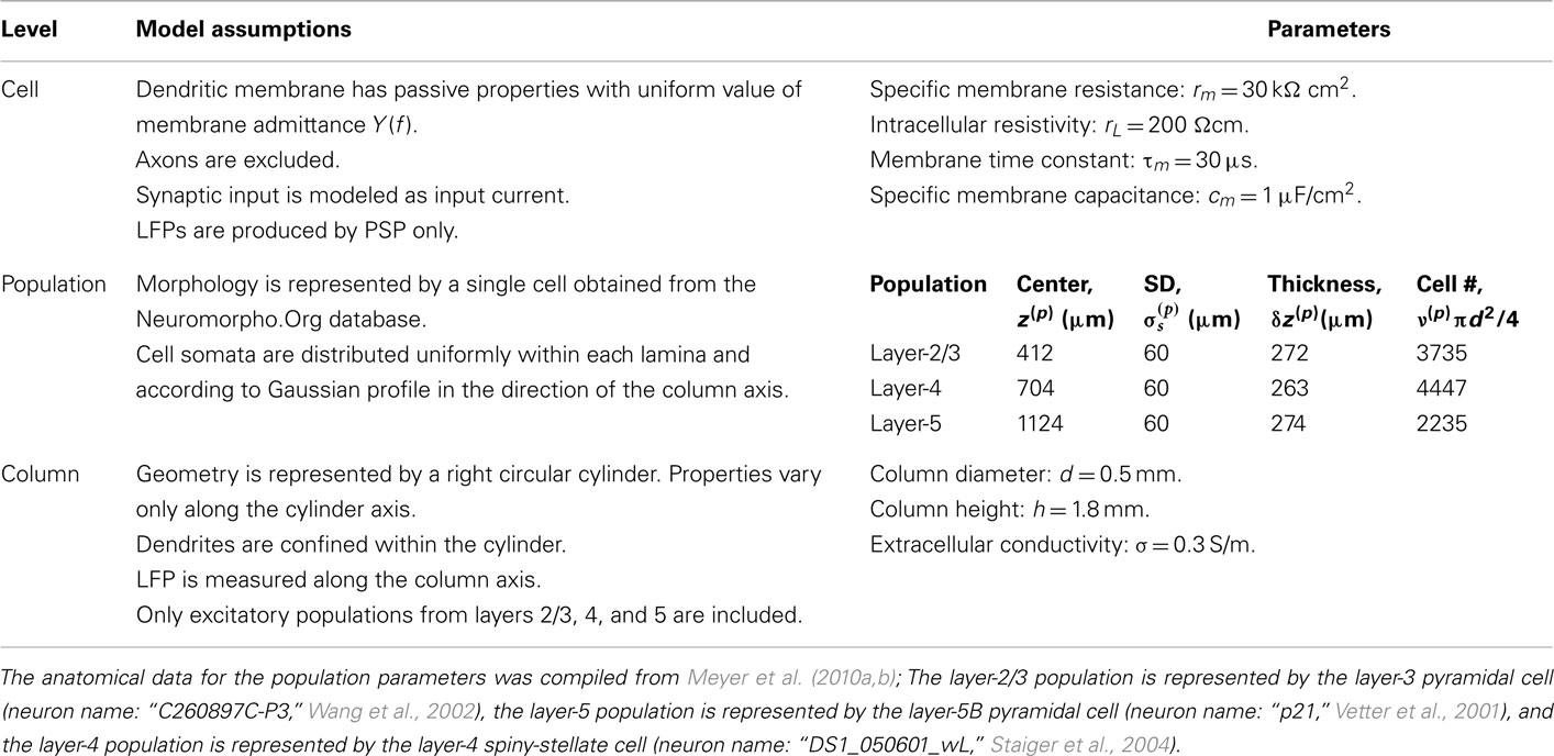
Table 1. Overview of the model at different levels of description.
Relationship between the extracellular potential and the CSD
Dendritic processing of synaptic inputs and the propagation of action potentials are accompanied by ionic currents flowing across the cell membrane and the surrounding tissue. The electromagnetic field associated with the currents of physiological origin satisfies the quasi-static condition (Plonsey and Heppner, 1967). When applied to a homogeneous extracellular medium with conductivity σ the quasi-static condition leads to the Laplace equation for the scalar field potential, Φ(r, t), with an effective solution (Plonsey, 1964; Geselowitz, 1967)
where the integration of the membrane current density Jm(r′, t) is performed over the membrane surface Am of all cells bounded by the volume under consideration. This expression tacitly assumes that the contribution of current density across the external boundary of the volume is negligible.
Neurons in cortical columns are arranged as collections of several tightly packed populations of morphologically and physiologically similar units activated by similar synaptic input. Therefore, on a spatial scale that is small in comparison to the distance |r − r′|, but sufficiently large to include portions of multiple neuritis within each elementary volume of tissue, the membrane currents can be described by a continuously distributed CSD (Nicholson, 1973):
where the transmembrane currents are summed over the membrane surface  of each n-th neurite contained within the elementary volume ΔV centered on position r. Consequently, the extracellular potential in Eq. 1 can be more conveniently expressed via a volume integral
over the CSD distribution within the tissue volume V.
Prediction of laminar LFP profiles evoked in response to input currents
The model linearity permits us to utilize the Green’s function method (Tuckwell, 1988) in order to express the p-th population laminar LFP, Φ(p)(z, t), evoked in response to an arbitrary transient laminar distribution of synaptic input currents,  per unit membrane area. The p-th population laminar LFP Green’s function, G(p)(z, ζ, t − t′), is defined as a population laminar LFP generated in response to a unit point input current delivered instantaneously at time t′ and applied to all dendritic compartments crossing a virtual plane oriented perpendicularly to the columnar axis and positioned a distance ζ from the soma of the respective cell. Then, the population LFP response to an arbitrary laminar distribution of input currents can be computed from
where the coordinate ζ is measured relative to the cell somata and spans the range [ζmin, ζmax] occupied by cell dendrites, while coordinate z is measured with respect to the pial surface. The complexity of dealing with the temporal dependence of the Green’s function can be avoided by analyzing the model in the frequency domain by taking the Fourier transform of Eq. 4:
where tilde (∼) represents the Fourier transforms of the corresponding variables from Eq. 4 at a particular frequency f.
For the numerical computations the integral in Eq. 5 is approximated using the midpoint rule, reducing the problem mathematically to the matrix product:

where complex-valued gain matrices  and the arrays of extracellular potentials
  and of synaptic input currents
  are evaluated at the locations zj = Δz/2 + (j − 1)Δz, Δz = h/Nj, j = 1, 2,…, Nj; and ζk = Δζ/2 + (k − 1)Δζ, Δζ = (ζmax − ζmin)/Nk, k = 1, 2,…, Nk. The Δz and Δζ are the depth discretization lengths for the pial-based and the soma-based coordinates, respectively, and were equally chosen at 20 μm.
The benefit of modeling the laminar LFP response to input currents in a frequency domain stems from the ability to compute the gain matrices  for each p-th population by applying compartmental neuron modeling in a Fourier domain, thus eliminating the simulations of the time-course of the dendritic response to a biophysically realistic synaptic input (see Population Laminar LFP Green’s Function in a Fourier Domain in Appendix). Finally, the gain matrix for the entire cortical column is constructed as a row of individual population gain matrices
  which is acting on the input currents to the corresponding populations combined into a column of arrays
  such that

which also includes a random noise array  to account for various aspects of model inadequacy.
Inverse Modeling: From LFP to Synaptic Input
Inverse problem
The inverse problem, in our case, is one of finding the frequency spectrum of the depth-distribution of synaptic input currents  from the Fourier transform of the recorded extracellular potential
  Since the number of channels recording the field potential is typically lower than the number of discrete points where synaptic currents are sought, the solution of the linear system is underdetermined and non-unique. This problem commonly arises in data analysis and, practically, the “best” solution is sought by minimizing the L2 norm of the residual
  and is given by the least squares solution
  where
where  is a Moore–Penrose pseudoinverse (Aster et al., 2005). Unfortunately, the pseudoinverse is commonly strongly ill-conditioned, i.e., small changes in measurements can lead to huge changes in the estimates, rendering the inverse solution extremely sensitive to the measurement noise. The inverse solution to the ill-posed problem can be stabilized by either selecting the minimum norm solution, as in Tikhonov regularization (Aster et al., 2005), or by enforcing a certain smoothness of the estimated input currents across the cortical depths as done here. The input currents are then estimated as

where  is the regularized inverse operator for estimating synaptic input currents (see Linear Inverse Operator for Estimation of Laminarly Smooth Input Currents in Appendix).
Insight regarding the constraints on the input current smoothness can be reached by examining the depth distributions of synaptic “innervation domains” obtained from the product of presynaptic axonal densities and the postsynaptic dendritic densities (Helmstaedter et al., 2007). For example, the innervation domain of presynaptic L2/3 axons on postsynaptic L2/3 cell dendrites produced by Feldmeyer et al. (2006) indicates that 80% of the integrated density of the synaptic contacts resides within a spatial region of about 200 μm when measured relative to the soma-centered reference frame. Since the magnitude of synaptic input is related to the density of innervations and the synaptic projections from individual populations are activated in unison, it is expected that the synaptic inputs to the population will be correlated on the scale of about 200 μm. The assumption of spatial covariance of the input currents can be effectively incorporated into the model by representing the laminar distribution of the population input currents as a linear combination

of a set of Nb “smooth” basis functions  where each column vector bm represents a m-th basis function which is spatially discretized at Nk equidistant locations; and β is a 1 × Nb array of weights specifying the contribution of each basis function to the input current. Consequently, the synaptic inputs can be reconstructed by estimating the contribution of each basis function to the reconstructed signal:

where  is now the regularized inverse operator for estimating contributions of each basis function (see Linear Inverse Operator for Estimation of Laminarly Smooth Input Currents in Appendix). Finally, the temporal dependence of the estimated synaptic inputs is obtained via the inverse Fourier transform:

Model resolution
The quality of the inverse solution can be characterized by assessing the model resolution matrix. From the definitions of the forward (Eq. 7) and inverse (Eq. 8) operators one obtains the relationship between the true and estimated synaptic currents:

where  is a model resolution matrix (Aster et al., 2005). Ideally, for well-conditioned problems and in the absence of measurement noise, the estimate must be equal to the correct value such that
  an identity matrix. However, by applying regularization, we sacrifice the details of the inverse solution in order to minimize the influence of the noise on the reconstructed solution. Each column (the resolution kernel)
  of the resolution matrix indicates how well the point synaptic input at the location ζk will be resolved in terms of synaptic inputs at all cortical depths. The resolution matrix is exclusively determined by properties of the forward model and the applied regularization technique and is independent from the specific data.
For the spatially correlated input currents, the resolution matrix, which measures the quality of the reconstruction of the point inputs, does not adequately judge the quality of the reconstruction provided by the inverse model. Instead we are interested in reconstructing the array of weights  specifying the contribution of each basis function to the input. The estimated weights
  are found by substituting Eq. 9 into Eq. 12 yielding

which indicates that the matrix  is a more adequate measure of the model resolution where each m-th column represents how well the basis function bmis reconstructed across the cortical depths.
Results
Modeling Laminar LFP Profiles: Single Population
Here, the methodology outlined in the Section “Materials and Methods” is applied to compute the frequency spectrum of the population laminar LFP Green’s functions. All simulations were carried out using MATLAB, which is well suited to matrix computations. Figure 1 shows the predicted population CSD and LFP laminar profiles evoked in response to localized excitatory (sink-like) steady-state currents applied at different positions relative to the soma of the layer-5 pyramidal cells. The CSD laminar profiles shown in the left column of Figure 1A indicate that the excitatory synaptic inputs to basilar dendrites initiate a strong localized current sink at the location of synaptic input accompanied by a spatially distributed return current sources (i.e., current entering the extracellular medium). The latter are the most prominent in the vicinity of the cell somata and at the apical tuft – the regions with the highest density of membrane area per unit cortical depth. Conversely, the excitatory input to the apical branch initiates the strong local sink there accompanied by the distributed return current sources most prominent along the apical branch itself and around the location of the soma. Despite the qualitative similarity, the CSD profiles in response to the synaptic inputs to the basilar versus apical dendrites are distinct from one another: (1) stronger return currents are manifested at the middle of the population in response to basilar rather than to apical stimulation; (2) the total excitatory input applied at the soma is stronger than that applied to the apical branch, because of the large somatic membrane area.
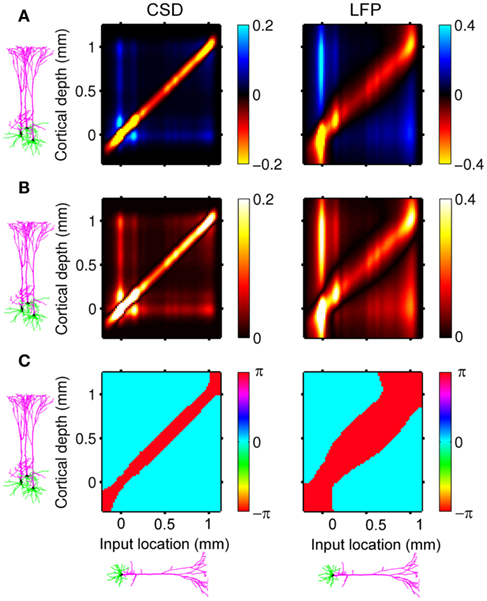
Figure 1. The predicted CSD (left) and the corresponding LFP (right) laminar profiles for the population of layer-5 pyramidal neurons in response to steady-state input current. The laminar profiles are computed as a function of the cortical depth relative to the position of the population center (vertical axis) in response to the point steady-state excitatory input current applied to cells at different vertical positions measured relative to the soma. The horizontally oriented cells depicted below each horizontal axis label identifies the locations of the synaptic input to the population, whereas the group of three vertically oriented cells depicted to the left of each vertical axis identifies the cell population with regard to the depth-distribution of the population laminar profiles. The real-valued laminar profiles (A) are also depicted as a combination of the absolute magnitude (B) and phase (C) used for complex-valued functions. The phase ψ = π corresponds to the inward currents on the CSD profile and the negative potential on the LFP profile. Relative units are used in (A,B): the color bars are normalized to 20 and 40% of the largest value of the CSD and the LFP, respectively.
The corresponding steady-state laminar LFP is shown in the right column of Figure 1A and manifests a pattern similar to the CSD but is spatially smoother due to the distal contributions of sources throughout the column to the LFP at a particular point along the column axis. In order to introduce the analysis of the complex-valued laminar profiles for non-zero frequencies, Figure 1 also shows the corresponding absolute magnitude (B) and the phase ψ (C) of the laminar profiles (A).
Figure 2 shows the absolute magnitude (A) and phase (B) of the predicted CSD and LFP laminar profiles at the frequencies of 10, 30, 100, and 250 Hz for the population of the layer-5 pyramidal cells. At non-zero frequencies the CSD also includes the capacitive current whose magnitude is proportional to the frequency of the input. In fact, the ratio of capacitive to leak currents, 2πfτm, is 1.9, 5.7, 18.9, and 47.1 for the frequencies of 10, 30, 100, and 250 Hz, respectively, in the cell having the membrane time constant τm = 30 ms. Therefore, for inputs at  , the dendritic processing is strongly dominated by the capacitive currents. The high amplitude of the CSD along the main diagonal in Figure 2A is dominated by the synaptic inputs with ψ ∼ π, as shown in Figure 2B. Conversely, the off-diagonal components of the laminar profiles correspond to the return currents, which decrease with distance from the location of the synaptic input. The phase of the return currents ψ ∼ 0 immediately outside the region of synaptic input and decreases monotonically farther out. Notably, for f > 100 Hz, the phase may approach that of the input current itself at some location on the tree. This implies that a cell driven with a sinusoidal current may have regions along the tree, where the return currents are flowing in-phase with the input current, unlike for the steady-state input, where input and return currents always flow in the anti-phase. The spectrum of the laminar LFP constitutes the spatially dissipated analog of the corresponding laminar CSD profiles, with a consequence that their phase advances more slowly with distance from the location of the synaptic input.
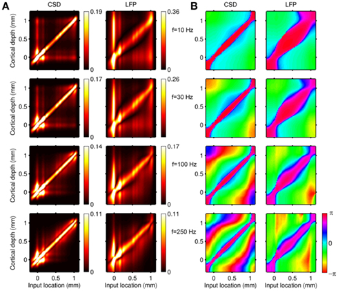
Figure 2. Predicted CSD and corresponding LFP laminar profiles for the population of layer-5 pyramidal neurons in response to sinusoidal input currents. The laminar profiles are computed as a function of the cortical depth (vertical axis) relative to the position of the population center, in response to the sinusoidal point input current oscillating at frequencies of 10, 30, 100, and 250 Hz applied to cells at different vertical positions measured relative to the soma. Complex-valued CSD and LFP profiles include both the absolute magnitude (A) and the phase (B). Relative units are used in (A): the color bars are normalized to 20 and 40% of the largest value of the CSD and the LFP, respectively and display the ratio of the largest value at a given frequency to that at the steady-state.
The computed laminar profiles clearly indicate the low-pass frequency-filtering of the LFP due to the electrical cable properties of dendrites (Pettersen and Einevoll, 2008; Lindén et al., 2010). The capacitive currents are stronger at higher frequencies, making cell membranes leakier, and consequently limiting the extent of dendritic processing to a more compact region around the location of the input, whereas the low-frequency input currents propagate farther away from the input. This leads to the reduction in the spatial separation of the input and return currents and their partial cancelation, producing weaker, and more compressed CSD/LFP laminar profiles as indicated by the colorbar scale in Figure 2A.
In order to appreciate the effect of the capacitive currents on the extracellular population response, Figure 3 compares the laminar profiles of the CSD and corresponding LFP from Figure 2 for inputs at a particular location x = 0.2 mm relative to the soma. The magnitudes of the CSD/LFP in the vicinity of the current input decrease progressively with increasing frequency of the input as a result of the larger contribution of the return currents acting in the anti-phase to the input, thus lowering the amplitude of the total current there. In contrast, the magnitude of membrane currents immediately outside the region of the current input is greater at higher frequencies due to stronger capacitive currents, leaving less current to pass to more distant dendritic branches. It is useful to compare the CSD and LFP responses to point input currents of the population of morphologically realistic cells to those of the population of finite parallel cables (discussed in Appendix) in order to discern the combined effects of cell morphology and scatter of cell somata around the population center on the evoked extracellular response.
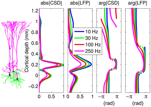
Figure 3. The predicted CSD and corresponding LFP laminar profiles from Figure 2 for current inputs applied at x = 0.2 mm relative to the cell soma at different frequencies. Complex-valued CSD and LFP profiles include both the absolute magnitude and the phase. Relative units are used such that the magnitude of the signal is normalized to that at the steady-state. The perceived discontinuity of the phase of the CSD is illusory because the phase is defined on the domain between −π and π.
Modeling Laminar LFP Profiles: Multiple Populations
Similarly to the population of the layer-5 pyramidal cell, the laminar profiles for the populations of the layer-2/3 pyramidal and layer-4 spiny-stellate cells were evaluated and assembled into a columnar laminar LFP response  Since the electrophysiological recordings measure the extracellular potential but not the CSD, only the LFP laminar profiles to the synaptic inputs will be presented in the following discussion.
Figure 4 shows the predicted laminar LFP Green’s functions of the modeled cortical column in response to the steady-state excitatory synaptic inputs. The differences in cell morphologies between the populations yield distinct features in their LFP laminar profiles: (1) The spatial extent of the laminar profiles is determined by the vertical span of the dendritic arbors, leading to very compact layer-4 LFP profile when compared to those for the populations of layer-2/3 and layer-5 pyramidal cells; (2) The magnitude of the laminar profiles depends on the density of the membrane area per unit laminar length, thus generating a much weaker response in the layer-4 spiny-stellate population in comparison to those in the pyramidal populations. Therefore the contribution of the layer-4 spiny-stellate population to the columnar LFP is overwhelmed by the contributions from pyramidal populations as demonstrated in Figure 4.
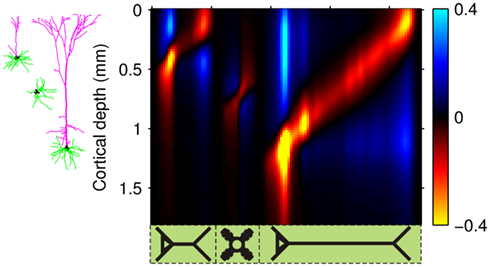
Figure 4. The predicted columnar LFP laminar profiles in response to steady-state inputs. The laminar profiles are computed as a function of the cortical depth relative to the position of the pial surface (vertical axis) in response to the point steady-state excitatory input current applied to cells in each population at different vertical positions measured relative to the soma (horizontal axis). The representative cell morphologies for each population are shown to the left of the LFP profiles and are positioned such that their somata are located at the centers of the corresponding population. The cartoon below the horizontal axis indicates the locations of synaptic inputs to cells in each modeled population, ordered from left to right as follows: L2/3, L4, and L5. Relative units are used such that the color bars are normalized to 40% of the largest LFP value.
Figure 5 shows the spectrum of the predicted columnar laminar LFP Green’s functions at the frequencies of 10, 30, 100, and 250 Hz. Here, the real, Re{LFP}, and imaginary, Im{LFP}, components of the columnar profiles are shown. The higher the frequency of the input the more out of phase the response becomes relative to the input, as indicated by the increasing imaginary component. The low-pass frequency-filtering of the LFP is again manifested by progressively more compressed laminar profiles for each population with the increasing frequency of the input. Notably, the relative contribution of the L4 population to the columnar LFP increases at higher frequencies. As a result of the low-pass filtering, the return currents leak out more proximal at higher frequencies, thus increasingly canceling the inputs in all cell types. However, in electrotonically compact cells the additional negation of input and return currents will have a lesser effect with increasing frequency, because there the currents already cancel strongly even for the steady-state condition.
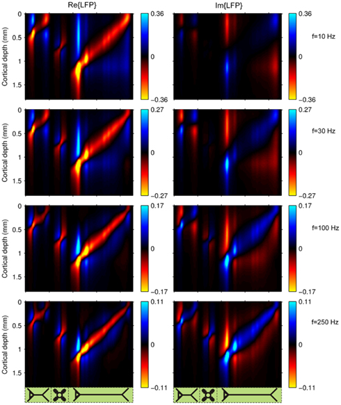
Figure 5. The predicted columnar LFP laminar profiles in response to sinusoidal input currents. The laminar profiles are computed as a function of the cortical depth relative to the position of the pial surface (vertical axis) in response to the sinusoidal point input current oscillating at frequencies of 10, 30, 100, and 250 Hz applied to cells in each population at different vertical positions measured relative to the soma (horizontal axis). The cartoon next to the horizontal axis indicates the locations of synaptic inputs to cells in each modeled population, ordered from left to right as follows: L2/3, L4, and L5. Relative units are used such that the color bars are normalized to 40% of the largest magnitude of the LFP at a particular frequency and display the ratio of the largest value at a particular frequency to that at the steady-state.
This effect is illustrated in Figure 6, which presents the frequency spectrum of the magnitude of the current-dipole moments evoked by each population in response to point inputs applied at different positions ζ, along the dendritic tree. Mathematically, they represent the magnitude of the equivalent current-dipole length  as a function of the point input location. The current-dipole moment in response to an arbitrary input profile can be found by integrating
  with the corresponding profile of the synaptic input (see CSD Green’s Function for a Population of Parallel Finite Linear Cables in Appendix). The magnitudes of
  for pyramidal populations have a strong peak in the vicinity of the soma and a smaller one at the apical branch, proportional to the laminar density of the membrane area. The longer L5-pyramidal cells evoke a stronger current-dipole moment than the L-2/3 pyramidal cells because the effective separation of the input and the return currents depends on the vertical extent of dendritic arbors. The dipole moment decreases sharply with the increasing frequency of the input for pyramidal populations, except in the population of compact spiny-stellate cells, in agreement with the above analysis of the LFP laminar profiles.
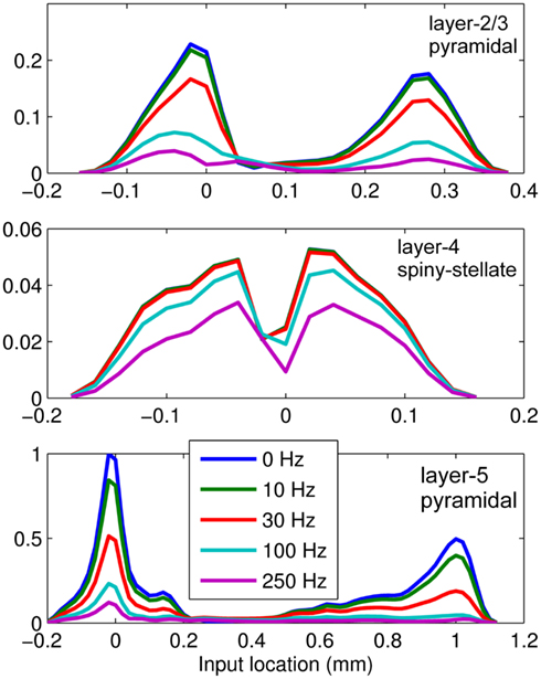
Figure 6. The differential effect of low-pass frequency-filtering on the modeled neuronal populations. The current-dipole moments evoked by each modeled population in response to point sinusoidal inputs oscillating at frequencies of 0, 10, 30, 100, and 250 Hz applied at different positions along the dendritic tree measured relative to the soma. All responses are normalized to the peak of the steady-state response of the layer-5 population.
Reconstruction of Synaptic Input: Single Population
The laminar profiles for the layer-5 cell population previously computed and presented in Figure 2 were used to generate the LFP data in response to hypothetical laminar distributions of synaptic input currents. The synthesized data was subsequently used to reconstruct the laminar distributions of hypothetical synaptic input, applying Eqs. 9 and 10. The specification of the inverse operator given by Eq. A13 requires a priori information about the basis functions’ smoothness  and the SNR level. For our computations we assume the SNR = 10.
Figure 7A shows the model resolution matrix  for frequency f = 30 Hz and the smoothness of the basis functions σb = 100 μm. Away from the end of the cell, a resolution matrix manifests the diagonal pattern such that most of the reconstructed signal power is concentrated in the narrow band centered on the main diagonal. However, the model does not reconstruct well the point inputs applied to the top or the bottom of the dendritic tree, as indicated by an increased contribution of the off-diagonal terms in the resolution matrix. As discussed in the Section “Materials and Methods,” a more adequate measure of the model resolution for spatially correlated inputs is represented by the transformed model resolution matrix
  presented in Figure 7B. It has a better-defined diagonal structure compared to the resolution matrix, indicating the adequacy of the inverse model. The imperfection of the model resolution manifested by the smooth resolution kernels around the location of the true input is a consequence of the regularization, and is the price paid to stabilize the solution against the effect of the random noise.
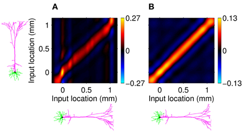
Figure 7. Assessment of the ability of the inverse model to reconstruct input currents to a single population from laminar LFP data assuming SNR = 10. The LFP data is generated by the population L5-pyramidal cells stimulated by the sinusoidal input currents oscillating at frequency f = 30 Hz and applied at different locations along the dendritic tree. (A) The model resolution matrix  as a measure of the reconstruction quality of point input currents, and (B) the transformed model resolution matrix
  as a measure of the reconstruction quality of smooth input currents with basis functions’ smoothness σb = 100 μm.
The effect of the smoothness of the basis function on the model resolution is investigated in Figure 8, showing the hypothetical and reconstructed laminar profiles of the synaptic inputs at f = 100 Hz applied to the layer-5 population. The reconstructed profiles were found using the inverse model with an assumed basis function smoothness σb = 100 μm. Figure 8A indicates that the inverse model does not reconstruct well the Gaussian synaptic input profiles with a standard deviation (SD) σt = 50 μm, which are spatially correlated on the scale shorter than that of the basis functions. Conversely, the shape of the synaptic inputs with σt = 150 μm is reconstructed perfectly, as seen in Figure 8B, because the assumed correlation length of the basis functions is shorter than that of the laminar distribution of synaptic inputs. Therefore, the specification of the basis functions smoothness parameter, σb, effectively establishes the resolution scale of the reconstructed synaptic inputs. More generally, Figure 8C shows the dependence of the root-mean-square error (RMSE) of the difference between the hypothetical and reconstructed synaptic input distributions as a function of the input smoothness, σt, for two choices of the basis function smoothness parameter: σb = 50 and 100 μm. The quality of reconstruction improves with the increasing width of the applied inputs for σt < σb and nearly plateaus at a small value when σt > σb, indicating that the inverse model reconstructs well the overall shape of the synaptic input whenever the input current smoothness parameter, σt, is greater than the basis functions smoothness parameter σb.
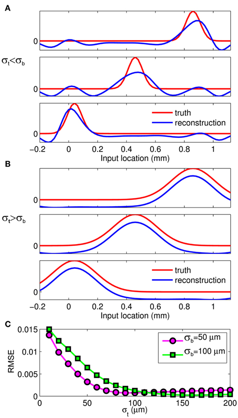
Figure 8. The effect of a priori smoothness of basis functions on the ability of the inverse model to reconstruct the laminar distribution of synaptic inputs to a single population assuming SNR = 10. The hypothetical (true) and reconstructed profiles of input currents at f = 100 Hz applied at different locations along the cells of the layer-5 population when input smoothness σt = 50 μm (A), and σt = 150 μm (B) and assuming basis function smoothness σb = 100 μm. (C) The RMSE of the difference between the hypothetical and reconstructed synaptic input distributions as a function of the input smoothness, σt, for two choices of the basis function smoothness: σb = 50 μm and σb = 100 μm.
The inverse model successfully reconstructs the overall shape of the hypothetical profiles; however, it is unable to reconstruct the mean level of applied synaptic current, as seen in Figure 8B, indicating that the forward model has a non-trivial null-space. Since an arbitrary laminar profile of the input current may be represented as the sum of a uniform component at the mean level of the synaptic input  and a component with zero mean
  it follows that the forward model has a null-space projection for uniform input currents, i.e.,
  making it impossible to reconstruct the mean level of synaptic activation across lamina. The physical cause for the existence of the null-space is easily understood for steady-state currents. A cell having a uniform specific membrane resistance stimulated with a uniform synaptic input current iin per unit membrane area will experience a shift in resting transmembrane potential by −iinrm in order to balance the input currents with the passive leak currents. The cell with an equipotential membrane, however, will produce zero axial and membrane currents, therefore generating no extracellular potential in response to such activation. Similarly, uniform sinusoidal currents applied to the cell having uniform membrane admittance will also result in zero membrane currents, as can be formally seen from Eq. A2. Indeed, the uniform distribution of the transmembrane voltage
  in all compartments will produce zero membrane current, i.e.,
  in each k-th compartment because ΣjMkj = 0. It follows from Eq. A3 that such a uniform distribution of transmembrane voltage is established when the membrane is uniformly stimulated by the current
  . Thus, the laminarly uniform component of the sinusoidal input current is projected to the null-space of the model and cannot be reconstructed without additional knowledge about the distribution of transmembrane voltage needed to fix the mean level of activation.
Reconstruction of Synaptic Input: Multiple Populations
Though the presence of the model null-space prevents reconstruction of the absolute profile of synaptic inputs, each cell population generates distinct laminar LFP profiles in response to synaptic inputs, thus suggesting that the inverse model may be used to discriminate the population origin of the evoked columnar LFP. In order to apply the modeled laminar LFP profiles shown in Figure 4 to the discrimination of the population origin of the LFP signal, it is necessary to properly constrain the laminar correlations of the synaptic input. The model assumes that the synaptic inputs are spatially correlated only within each population and are uncorrelated between different populations. The assumed basis functions’ smoothness is σb = 50 μm for the L2/3 and L4 populations and σb = 100 μm for the L5 population.
The performance of the inverse model is demonstrated in Figure 9, which compares the hypothetical (A) and reconstructed (B,C) laminar profiles of synaptic input currents applied at frequency f = 30 Hz, assuming the SNR of 10 and 1000, respectively. The input smoothness in Figure 9A σt = 75 μm for the L2/3 and L4 populations and σt = 150 μm for the L5 population. Due to the linearity of the problem, the more general case of currents applied to several populations simultaneously can be obtained by the linear superposition of these basic current inputs. Similarly to the single population case, the model is fundamentally incapable of reconstructing the mean level of the synaptic input applied to each population as indicated by the zero-mean level of reconstructed laminar profiles in Figures 9B,C. Nevertheless, the inverse model successfully identifies the population-specific synaptic inputs with the limited mis-assignment of the reconstructed synaptic inputs to the other two populations. The mis-assignment largely occurs between spatially overlapping regions of each population. For example, the hypothetical inputs applied to the L2/3 population are reconstructed as the inputs to the L2/3 population with the partial input to the L5 population applied at the same cortical depth and vice versa. On the other hand the true inputs to the L4 population are reconstructed with the minimal mis-assignment to the L2/3 population because of the minimal overlap between the two populations. Unlike the ambiguity regarding the mean level of the laminar profiles of synaptic input which results from the model null-space, the mis-assignment ambiguity results from the regularization of the inverse operator. Figure 9C indicates that the mis-assignment ambiguity is strongly diminished for negligible levels of noise and therefore does not fundamentally limit the reconstruction of synaptic inputs.

Figure 9. The assessment of the ability of the inverse model to reconstruct the distribution of the population-specific spatially smooth synaptic inputs from the composite LFP data. The hypothetical laminar profiles (A) of synaptic input currents oscillating at frequency f = 30 Hz applied at different locations along the dendritic tree to each population. The input smoothness σt = 75 μm for the L2/3 and L4 populations and σt = 150 μm for the L5 population. The corresponding reconstructed laminar profiles of synaptic input assuming the SNR of 10 (B) and 1000 (C). The assumed basis functions’ smoothness: σb = 50 μm for the L2/3 and L4 populations and σb = 100 μm for the L5 population. The location of the input corresponds to the position of the matrix column relative to the cartoon shown below the horizontal axis, whereas the cartoon next to the vertical axis indicates the partitioning of the matrix column elements between different populations.
Similarly to the single population analysis, Figure 10A shows the dependence of the RMSE of the difference between the hypothetical and reconstructed synaptic input distributions as a function of the input smoothness for two choices of the basis function smoothness parameter σb = 50 and 100 μm. Again, the dissimilarity decreases with the increasing width of the applied inputs when σt < σb and nearly plateaus when σt > σb. The hypothetical and reconstructed profiles are less similar in the column than in a single population because of the presence of the mis-assignment. Figures 10B,C shows the signal power resolution matrices for the modeled column computed from Figures 9B,C, respectively, in which each column represents the normalized power distribution of the reconstructed signal among each population when inputs are applied to a particular population. The perfect resolution matrix would correspond to the identity matrix. However, the presence of the limited mis-assignment as described above deposits some signal power into the overlapping cortical populations. Figure 10B shows that at the SNR = 10, the strongest mis-assignment occurs for inputs to the L2/3 population, which are reconstructed as a combination of inputs to the L2/3 (82%) and the L5 (18%), whereas, the inputs to the L4 and L5 populations are reconstructed with the proper assignment of the signal power at the levels of 93 and 98%, respectively. When the noise level is negligible (e.g., SNR = 1000) the decomposition of LFP signal is nearly perfect as shown in Figure 10C. Nonetheless, at a finite level of noise, the presence of the spatial overlap between populations prevents a fully unambiguous decomposition of the LFP into activity of individual populations without additional information about the distribution of synaptic innervations.
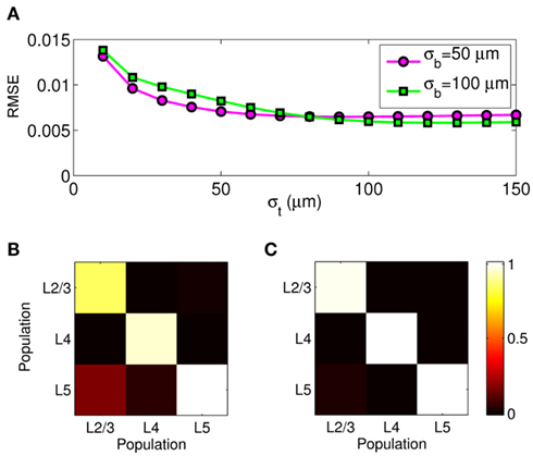
Figure 10. Assessment of the ability of the inverse model to decompose the composite columnar LFP into population-specific contributions assuming spatially smooth laminar distribution of synaptic inputs applied at f = 30 Hz. (A) The RMSE of the difference between the hypothetical and reconstructed synaptic input distributions, as a function of the input smoothness, σt, for two choices of the basis function smoothness: σb = 50 μm and σb = 100 μm. (B,C) The signal power resolution matrix for the modeled column computed from Figures 9B,C, respectively. Each column represents the normalized distribution of the power of the reconstructed signal among each population when inputs are applied to a particular population.
Reconstruction of Population Activity Based on Synaptic Innervation Anatomy
The inverse model can be significantly constrained by incorporating into the model the anatomical information about the laminar distribution of the density of synaptic innervation between the populations. The synaptic innervation densities for the canonical cortical microcircuit of excitatory synaptic projections were obtained by Lübke and Feldmeyer (2007); (see their Figure 7) from the product of the presynaptic axonal densities and the postsynaptic dendritic densities. This includes L4-to-L4, L4-to-L2/3, L2/3-to-L2/3, L2/3-to-L5, and L5-to-L5 synaptic projections.
The density of synaptic innervation uniquely determines the basis functions for input currents. Input currents may again be expressed via Eq. 9, where the matrix of basis functions B = [b1; …;  ] is now composed of a set of synaptic innervations density profiles and β is a 1 × Nb array of normally distributed with zero mean, uncorrelated weights specifying the strength of the corresponding synaptic projection, and needs to be found from the inverse solution. The anatomical data from Lübke and Feldmeyer (2007) was utilized to simulate the laminar response of the modeled cortical populations having the representative cell morphologies shown in Figure 11A. The digitized depth distributions of anatomical innervation domains are presented in Figure 11B, and the corresponding LFP responses of cortical populations at frequency f = 30 Hz of synaptic input are depicted in Figure 11C.
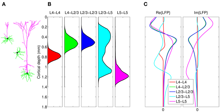
Figure 11. Modeling of the population-specific laminar LFP profiles in response to activation of anatomically realistic excitatory synaptic projections. (A) Representative morphologies of the cells in the modeled populations; (B) the digitized innervation domains for each projection from Figure 7 of Lübke and Feldmeyer (2007); (C) the corresponding complex-valued modes of the LFP response to sinusoidal inputs oscillating at f = 30 Hz. The somata of representative cells are properly aligned with the depth-distribution of the innervation domains. The innervation domains are displayed normalized to their peak values.
Figure 12A shows the resolution matrix for the constrained model where each column represents how well the activation of a particular synaptic project will be resolved in terms of all modeled projections. The model discriminates very well between synaptic projections except for those to the L2/3, where the reconstruction almost equally assigns the contribution to either projection from the presynaptic L4 or L2/3 populations. This result is expected because the laminar profiles of both L4-to-L2/3 and L4-to-L4 innervation densities are very similar and therefore produce almost identical LFP, as demonstrated in Figure 11C. In contrast, the synaptic projections to the L5 population are well discriminated between those arriving from the L2/3 or L5 population because of the strong differences in the respective profiles of synaptic innervation densities. The role of the differences between the synaptic innervation domains on the ability to reconstruct the population activity can be demonstrated by combining the synaptic clouds projecting from L2/3 and L4 toward the L2/3 into a single innervations domain projecting toward the L2/3 population in the model. The resolution matrix for such a model is shown in Figure 12B and indicates a robust discrimination of the modeled synaptic projections. The quality of the resolution is lowest for the identification of the L4-to-L4 projection with a corresponding diagonal element of the resolution matrix 0.83, whereas the diagonal elements for the other projections exceed 0.99, indicating an excellent model resolution. The LFP signal evoked by the population of spatially compact L4 spiny-stellate cells is much weaker than that evoked by the L2/3 and L5 populations of pyramidal cells in response to the synaptic input. Consequently, the signal from the spiny-stellate cells is overshadowed by that of the pyramidal populations, making reconstruction by the inverse model more difficult.
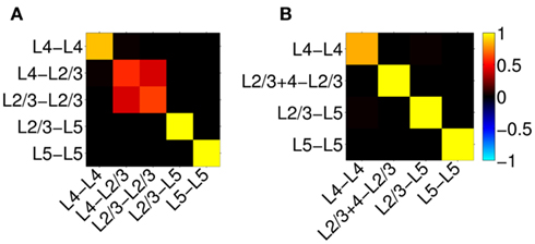
Figure 12. Assessment of the ability of the inverse model to disambiguate the activated synaptic projection from composite LFP signal assuming a priori knowledge of the spatial distribution of synaptic connectivity shown in Figure 11C and SNR = 10. The resolution matrices for two cases: (A) all known projections are included, and (B) projections L4-to-L2/3 and L2/3-to-L2/3 are combined into a single synaptic projection L2/3 + 4-to-L2/3. Each column of the matrix represents the ability of the inverse model to properly reconstruct the contribution of each synaptic projection to the evoked LFP signal at the frequency of input f = 30 Hz.
Reconstruction of Synaptic Inputs from Experimental LFP Data
In order to illustrate the utility of the proposed method for interpreting electrophysiological recordings, we here reconstruct the population-specific laminar profiles of synaptic inputs from experimental LFP data. We use the data from Einevoll et al. (2007) collected with a linear multielectrode with 23 channels spaced at 0.1 mm and inserted perpendicularly to the pial surface into the somatosensory cortex of the anesthetized rat. The recorded potential was evoked in response to deflection of a single whisker. For the purpose of this demonstration, we focused on a single stimulus condition (rise time: t1, amplitude: a1 from the experiment #1 in Einevoll et al., 2007). The recorded laminar-electrode potential was amplified and analogically filtered online into two signals: a low-frequency part and a high-frequency part. Only the low-frequency part (0.1–500 Hz), sampled at 2 kHz with 16 bits (Ulbert et al., 2001) was used in the present analysis.
Figure 13A depicts the representative cell morphologies in the modeled populations and the anatomical structure of the modeled cortical column used to reconstruct the activated synaptic projections from laminar LFP data. Figure 13B presents the stimulus averaged LFP data for 60 ms following the stimulus onset and shows a simple laminar structure: positive between 0 and 0.2 mm and negative elsewhere during its strongest episode between 20 and 30 ms. In order to eliminate the influence of the potential variation at the reference electrode positioned on the skull, the mean potential across all electrodes was subtracted from all contacts at each timepoint. Figure 13C shows the laminar profiles of the reconstructed population-specific synaptic inputs which were obtained by (1) Fourier transforming the LFP data into a frequency domain; (2) Estimating the contribution of each basis function to the reconstructed synaptic inputs by applying the inverse model in a frequency domain via Eq. 10; and (3) Fourier transforming the frequency spectrum of reconstructed synaptic inputs back into a temporal domain via Eq. 11. The inverse operator was constructed with the assumed SNR = 10 and the basis functions’ smoothness σb = 50 μm for the L2/3 and L4 populations and σb = 100 μm for the L5 population.
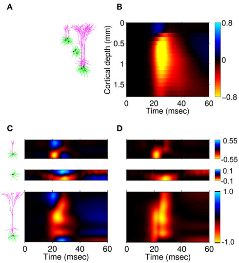
Figure 13. Model application to the reconstruction of synaptic inputs from experimental LFP data. Representative cell morphologies in the modeled populations and the anatomical structure of the modeled cortical column (A); and the corresponding depth distribution of the experimental LFP data from Einevoll et al. (2007)(B). The estimated population-specific laminar profiles of synaptic input (C) obtained by applying the inverse model to the experimental LFP data. The cell morphologies next to the vertical axis indicate the laminar input locations to the cells in each modeled population. (D) The estimated population-specific laminar profiles of synaptic input assuming a strictly excitatory inputs. Relative units normalized to the maximum of the reconstructed current are used.
As previously emphasized, the inverse model is unable to reconstruct the mean level of synaptic inputs. However, since it is assumed that the LFP signal is largely generated by the excitatory columnar network, each of the population-specific profiles of synaptic inputs can be uniformly shifted so as to render all currents negative (excitatory) as depicted in Figure 13D. The earliest excitation is projected to layer-4 followed by the synaptic input to layer-2/3 and layer-5 populations. Strong input to the layer-2/3 pyramidal population is initiated at the basilar dendrites and is succeeded by a weaker input to the apical branch. In contrast, the input to the layer-5 pyramidal population is applied to almost the entire dendritic tree. Such a pattern of the laminar distribution of the population-specific excitatory synaptic inputs is generally consistent with the innervation anatomy depicted in Figure 11B and with the predictions of the LPA (Einevoll et al., 2007). The LFP signal 30 ms after the stimulus onset and the corresponding estimated currents are presumably generated by the activity of electrogenic Na+/K+ pumps (not included in this model), which explains the opposite polarity of these currents with respect to synaptic inputs activated during 20–30 ms time window.
Discussion
In the present study, we introduced a novel mathematical framework for reconstructing population-specific synaptic inputs from laminar LFP recordings, extending beyond the CSD analysis. Our approach involves a combination of the forward model, which predicts population laminar LFP profiles in response to synaptic input applied at different locations along the cells, and the inverse model, which reconstructs synaptic inputs from the laminar LFP data based on the forward prediction. Assuming spatial correlation of synaptic inputs within but not between neuronal populations, the model decomposes the columnar LFP profile into population-specific contributions. Constraining the solution with a priori knowledge of spatial distribution of synaptic connectivity further allows prediction of activated synaptic projections from the columnar LFP measurements.
Forward Modeling
In the current modeling approach, neurons have passive dendritic trees and no axons, synaptic inputs are modeled as input currents rather than via voltage-dependent conductance changes, and LFPs are generated by excitatory synaptic inputs only. This set of simplifications leads to a fully linear forward model and allows analysis of the problem via the Green’s function approach in the Fourier domain. The procedure for simulating the columnar LFP profiles, i.e., LFP Green’s functions, is composed of the following steps: (1) compute the net transmembrane current distributions from the representative cells in response to input currents injected at different cortical depths relative to their somata by applying compartmental neuron modeling in a Fourier domain; (2) compute the population CSD and respective LFP laminar profiles in response to synaptic inputs from the transmembrane current responses of the representative cell; (3) construct columnar LFP laminar profiles from those of individual populations.
In agreement with previous work conducted for individual cells (Pettersen and Einevoll, 2008; Lindén et al., 2010), we found low-pass frequency-filtering of the population LFP signatures due to the electrical cable properties of dendrites. The effect is manifested by the compression and weakening of the LFP laminar profiles in response to input currents at higher frequencies. Consequently, the synaptic input with, for instance, uniform distribution of spectral power will generate low-passed spectral distribution of LFP signal in a homogeneous and purely resistive extracellular medium. The same conclusions can be drawn from the analysis of the population current-dipole moments evoked in response to the point sinusoidal inputs at different frequencies, shown in Figure 6, indicating a strong reduction in magnitude with increasing frequency of input.
The predicted laminar LFP profiles for the modeled populations have distinct features stemming from the morphological differences between the cell populations. Crucially, the span of dendritic arborization determines the spatial extent of the LFP profiles, whereas the laminar density of the membrane area determines their magnitude. For this reason, at a steady-state, the LFP profile of the large layer-5 pyramidal population is much stronger than that of the population of compact layer-4 spiny-stellate cells. However, as frequency of input increases, the length of dendritic arborization becomes less important, because most return currents leave cells in the vicinity of the current input and do not propagate to the distant dendritic arbors. This effect has the strongest impact on pyramidal populations and increases the relative contribution of layer-4 spiny-stellate population to the total LFP signal at higher frequencies.
The current model only considers variation of extracellular potential along the axis of a cortical column. Thus, although each population is represented only by a single reconstructed cell, the specifics of the dendritic geometry of the chosen representative cell in any but the axial plane do not affect the forward solution. In addition, the implemented normal distribution of population elements along the columnar axis further reduces the field variation specific to the particular chosen morphologies.
Inverse Modeling
Inversion of hypothetical laminar LFP recordings is performed using a regularized linear estimation method requiring a priori specification of the noise and signal covariance at different laminar locations of synaptic input. The inverse model reconstructs perfectly the shape of the hypothetical laminar distributions of synaptic input which are spatially smooth on the scale of the correlation length σb specified by the a priori basis functions. Thus, the a priori correlation length must be shorter than the correlation scale of the realistic synchronous synaptic inputs in order guarantee the applicability of the model.
The assumption in the inverse model about spatial correlation between the inputs at different laminar depths implies that the reconstructed synaptic input profiles cannot include spatial wavelengths on the order shorter than correlation length σb, which determines the spatial resolution of the reconstructed input currents. Constraining the spatial resolution of the reconstructed input is essential to ensure the stability and the validity of the inverse solution. The forward model does not include highly detailed spatial scale: wavelengths shorter than  are filtered out in the process of constructing the population laminar CSD profiles via Eq. A6, and then further as a result of computing the spatially disperse laminar LFP profiles via the convolution operator in Eq. A7. At the same time, short wavelengths in the data largely reflect information about specific details of the underlying neuronal morphologies, which is not accounted for in the forward model. Therefore, wavelengths shorter than the smallest spatial scale captured by the forward model need to be suppressed in order to stabilize the inverse solution. As long as the a priori correlation length is larger than the smallest spatial scale in the forward model, the inverse model will reconstruct the input profiles consistent with the a priori constraints. The anatomical measurements suggest that synchronous synaptic inputs strongly correlate on the scale of about 200 μm (Feldmeyer et al., 2006), larger than the resolution of the forward model,
  , which provides considerable range in the choice of the a priori correlation length ensuring the validity of the presented model for realistic biophysical applications.
The inverse model is inherently incapable of reconstructing the absolute magnitude of the input currents and produces the zero-mean laminar input current distributions, indicating that the mean level of the input across different cortical depths is projected onto the null-space of the forward model. However, the null-space may be avoided entirely by uniquely specifying basis functions for activation of each modeled synaptic projection based on anatomical data. Applied uniform input current per unit membrane merely shifts the resting transmembrane potential in the cell, resulting in zero axial currents and no extracellular response, i.e., the extracellular potential does not mirror the spatial average of the transmembrane potential and therefore cannot be directly used to measure the degree of depolarization of cells in the population. The inability of the inverse model to reconstruct the uniform component of input currents is contingent upon the particular model assumption of having uniform impedance across the cell membrane. For non-uniform membrane properties, more generally, it is the current distribution,  that cannot be reconstructed by the inverse model, where Yj(f ) is the membrane impedance of j-th compartment. In either case, the presence of the null-space prevents the complete reconstruction of the input currents.
Notwithstanding the presence of the null-space, the distinct features of each population laminar LFP permit discrimination of the population origin of evoked columnar LFP, provided we assume that synaptic inputs are spatially correlated only within each population. The spatial overlap between the populations across the column is responsible for a partial mis-assignment of the reconstructed signal and requires additional anatomical constraints to discriminate the population origin of the evoked LFP.
The anatomical data about the laminar distribution of synaptic innervation domains eliminates the null-space ambiguity by uniquely constraining the basis functions and reducing the dimensionality of the inverse model to the number of included synaptic projections. Such an inverse model successfully identifies the activated synaptic projections from the LFP data, provided that the population LFP laminar profiles in response to each synaptic projection are dissimilar from one another.
Previously, Einevoll et al. (2007) demonstrated that by incorporating cell-type specific morphologies the LPA can be extended to estimate the synaptic projections between the identified populations while assuming that the columnar LFP is evoked by the firing of modeled neuronal populations measured by the MUA in the same column. However, this cannot always be the case, as long-distance axonal projections impinging on the column, generally, will also contribute to the LFP. In contrast, the current model does not require the MUA data and can incorporate the anatomical information on a synaptic connection regardless of the origin of the presynaptic populations.
Implications and Future Directions
The current framework is limited inasmuch as it considers only the populations of excitatory layer-2/3 and layer-5 pyramidal and layer-4 spiny-stellate cells, each modeled by a single representative morphology, and as it assigns only passive properties to dendrites. Nevertheless, the model successfully delineates the key relationships between the synaptic inputs and the evoked LFP and will serve as a foundation for a more realistic modeling of extracellular potential in the cortical column. In a more comprehensive model, the active dendritic properties can be included via linearization of the voltage-dependent current, resulting in inductance-like terms in the equations describing the dendritic processing of the input currents (Koch, 1999); whereas, the electrogenic Na+/K+ pump currents can be modeled by coupling the membrane current balance equation with the equations for the conservation of the Na+ and K+ ions (Karbowski, 2009). The additional cell populations, which might additionally contribute to the LFP signal, can be included as their morphological reconstructions become readily available.
One way to resolve the ambiguity caused by the null-space in the population-specific laminar distribution of synaptic input currents is to augment the extracellular recordings with the corresponding measurements of the mass transmembrane voltage, e.g., by using a voltage-sensitive dye (VSD) technique. Alternatively, the zero-mean ambiguity in the laminar distribution of synaptic input caused by the null-space may be resolved if the synaptic input is positively identified as either excitatory or inhibitory. This information can be obtained from the population firing-rate model, which seeks the optimal pattern of excitation/inhibition transfer between the populations and corresponding model parameters by assimilating the experimentally extracted firing rates (Blomquist et al., 2009).
Here, we present a case for the interpretation of LFP data in terms of synaptic projections between neuronal populations based on biophysical rather than mathematical constraints. Notably, our approach represents a novel synthesis of two types of anatomical information (cell morphologies and synaptic innervation domains) integrated into a unified computational model to explore synaptic activity of cortical populations based on multielectrode extracellular recordings. Recent trends including growing public availability of reconstructed morphologies (Ascoli, 2006) and interest in mapping the synaptic connections of the brain (Helmstaedter et al., 2007; Lichtman and Sanes, 2008) provide significance and viability to our modeling approach.
Conflict of Interest Statement
The authors declare that the research was conducted in the absence of any commercial or financial relationships that could be construed as a potential conflict of interest.
Acknowledgments
This work was supported by NIH Grants R01-EB000790, R01-NS051188, R21-EB009118, R01-NS057198, and the Research Council of Norway (eScience). We are thankful to P. C. Hansen for making freely available the Regularization Toolbox (www.imm.dtu.dk/∼pch/Regutools/) and for helpful suggestions.
Footnotes
References
Ascoli, G. A. (2006). Mobilizing the base of neuroscience data: the case of neuronal morphologies. Nat. Rev. Neurosci. 7, 318–324.
Ascoli, G. A., Donohue, D. E., and Halavi, M. (2007). NeuroMorpho.Org: a central resource for neuronal morphologies. J. Neurosci. 27, 9247–9251.
Aster, R., Borchers, B., and Thurber, C. (2005). Parameter Estimation and Inverse Problems. Amsterdam: Academic Press.
Blomquist, P., Devor, A., Indahl, U. G., Ulbert, I., Einevoll, G. T., and Dale, A. M. (2009). Estimation of thalamocortical and intracortical network models from joint thalamic single-electrode and cortical laminar-electrode recordings in the rat barrel system. PLoS Comput. Biol. 5, e1000328. doi:10.1371/journal.pcbi.1000328
Csicsvari, J., Henze, D. A., Jamieson, B., Harris, K. D., Sirota, A., Barthó, P., Wise, K. D., and Buzsáki, G. (2003). Massively parallel recording of unit and local field potentials with silicon-based electrodes. J. Neurophysiol. 90, 1314–1323.
Dale, A. M., and Sereno, M. I. (1993). Improved localizadon of cortical activity by combining EEG and MEG with MRI cortical surface reconstruction: a linear approach. J. Cogn. Neurosci. 5, 162–176.
Dayan, P., and Abbott, L. F. (2001). Theoretical Neuroscience: Computational and Mathematical Modeling of Neural Systems, 1st Edn. Cambridge, MA: MIT Press.
Di, S., Baumgartner, C., and Barth, D. S. (1990). Laminar analysis of extracellular field potentials in rat vibrissa/barrel cortex. J. Neurophysiol. 63, 832–840.
Einevoll, G. T., Pettersen, K. H., Devor, A., Ulbert, I., Halgren, E., and Dale, A. M. (2007). Laminar population analysis: estimating firing rates and evoked synaptic activity from multielectrode recordings in rat barrel cortex. J. Neurophysiol. 97, 2174–2190.
Feldmeyer, D., Lübke, J., and Sakmann, B. (2006). Efficacy and connectivity of intracolumnar pairs of layer 2/3 pyramidal cells in the barrel cortex of juvenile rats. J. Physiol. (Lond.) 575, 583–602.
Fries, P., Reynolds, J. H., Rorie, A. E., and Desimone, R. (2001). Modulation of oscillatory neuronal synchronization by selective visual attention. Science 291, 1560–1563.
Gail, A., Brinksmeyer, H. J., and Eckhorn, R. (2004). Perception-related modulations of local field potential power and coherence in primary visual cortex of awake monkey during binocular rivalry. Cereb. Cortex 14, 300–313.
Geselowitz, D. B. (1967). On bioelectric potentials in an inhomogeneous volume conductor. Biophys. J. 7, 1–11.
Gustafsson, B. (1984). Afterpotentials and transduction properties in different types of central neurones. Arch. Ital. Biol. 122, 17–30.
Halgren, E., Wang, C., Schomer, D. L., Knake, S., Marinkovic, K., Wu, J., and Ulbert, I. (2006). Processing stages underlying word recognition in the anteroventral temporal lobe. Neuroimage 30, 1401–1413.
Hasenstaub, A., Shu, Y., Haider, B., Kraushaar, U., Duque, A., and McCormick, D. A. (2005). Inhibitory postsynaptic potentials carry synchronized frequency information in active cortical networks. Neuron 47, 423–435.
Helmstaedter, M., de Kock, C. P. J., Feldmeyer, D., Bruno, R. M., and Sakmann, B. (2007). Reconstruction of an average cortical column in silico. Brain Res. Rev. 55, 193–203.
Kamondi, A., Acsády, L., Wang, X. J., and Buzsáki, G. (1998). Theta oscillations in somata and dendrites of hippocampal pyramidal cells in vivo: activity-dependent phase-precession of action potentials. Hippocampus 8, 244–261.
Karbowski, J. (2009). Thermodynamic constraints on neural dimensions, firing rates, brain temperature and size. J. Comput. Neurosci. 27, 415–436.
Koch, C. (1999). Biophysics of Computation: Information Processing in Single Neurons, 1st Edn. Oxford: Oxford University Press.
Leski, S., Kublik, E., Swiejkowski, D. A., Wróbel, A., and Wójcik, D. K. (2009). Extracting functional components of neural dynamics with independent component analysis and inverse current source density. J. Comput. Neurosci. 29, 459–473.
Lichtman, J. W., and Sanes, J. R. (2008). Ome sweet ome: what can the genome tell us about the connectome? Curr. Opin. Neurobiol. 18, 346–353.
Lindén, H., Pettersen, K. H., and Einevoll, G. T. (2010). Intrinsic dendritic filtering gives low-pass power spectra of local field potentials. J. Comput. Neurosci. 29, 423–444.
Liu, A. K., Dale, A. M., and Belliveau, J. W. (2002). Monte Carlo simulation studies of EEG and MEG localization accuracy. Hum. Brain Mapp. 16, 47–62.
Lübke, J., and Feldmeyer, D. (2007). Excitatory signal flow and connectivity in a cortical column: focus on barrel cortex. Brain Struct. Funct. 212, 3–17.
Mainen, Z. F., and Sejnowski, T. J. (1998). “Modeling active dendritic processes in pyramidal neurons,” in Methods in Neuronal Modeling, 2nd Edn, From Ions to Networks eds C. Koch and I. Segev (Cambridge, MA: The MIT Press), 171–210.
Makarov, V. A., Makarova, J., and Herreras, O. (2010). Disentanglement of local field potential sources by independent component analysis. J. Comput. Neurosci. 29, 445–457.
Meyer, H. S., Wimmer, V. C., Hemberger, M., Bruno, R. M., de Kock, C. P. J., Frick, A., Sakmann, B., and Helmstaedter, M. (2010a). Cell type–specific thalamic innervation in a column of rat vibrissal cortex. Cereb. Cortex 20, 2287–2303.
Meyer, H. S., Wimmer, V. C., Oberlaender, M., de Kock, C. P. J., Sakmann, B., and Helmstaedter, M. (2010b). Number and laminar distribution of neurons in a thalamocortical projection column of rat vibrissal cortex. Cereb. Cortex 20, 2277–2286.
Mitzdorf, U. (1985). Current source-density method and application in cat cerebral cortex: investigation of evoked potentials and EEG phenomena. Physiol. Rev. 65, 37–100.
Nicholson, C. (1973). Theoretical analysis of field potentials in anisotropic ensembles of neuronal elements. IEEE Trans. Biomed. Eng. 20, 278–288.
Nicholson, C., and Freeman, J. A. (1975). Theory of current source-density analysis and determination of conductivity tensor for anuran cerebellum. J. Neurophysiol. 38, 356–368.
Nicholson, C., and Llinas, R. (1971). Field potentials in the alligator cerebellum and theory of their relationship to Purkinje cell dendritic spikes. J. Neurophysiol. 34, 509–531.
Nunez, P. L., and Srinivasan, R. (2006). Electric Fields of the Brain: The Neurophysics of EEG. Oxford: Oxford University Press.
Pesaran, B., Pezaris, J. S., Sahani, M., Mitra, P. P., and Andersen, R. A. (2002). Temporal structure in neuronal activity during working memory in macaque parietal cortex. Nat. Neurosci. 5, 805–811.
Pettersen, K. H., Devor, A., Ulbert, I., Dale, A. M., and Einevoll, G. T. (2006). Current-source density estimation based on inversion of electrostatic forward solution: effects of finite extent of neuronal activity and conductivity discontinuities. J. Neurosci. Methods 154, 116–133.
Pettersen, K. H., and Einevoll, G. T. (2008). Amplitude variability and extracellular low-pass filtering of neuronal spikes. Biophys. J. 94, 784–802.
Pettersen, K. H., Hagen, E., and Einevoll, G. T. (2007). Estimation of population firing rates and current source densities from laminar electrode recordings. J. Comput. Neurosci. 24, 291–313.
Plonsey, R., and Heppner, D. B. (1967). Considerations of quasi-stationarity in electrophysiological systems. Bull. Math. Biophys. 29, 657–664.
Schroeder, C. E., Mehta, A. D., and Givre, S. J. (1998). A spatiotemporal profile of visual system activation revealed by current source density analysis in the awake macaque. Cereb. Cortex 8, 575–592.
Segev, I., and Burke, R. E. (1998). “Compartmental models of complex neurons,” in Methods in Neuronal Modeling, 2nd Edn, From Ions to Networks, eds C. Koch and I. Segev (Cambridge, MA: MIT Press), 93–136.
Staiger, J. F., Flagmeyer, I., Schubert, D., Zilles, K., Kötter, R., and Luhmann, H. J. (2004). Functional diversity of layer IV spiny neurons in rat somatosensory cortex: quantitative morphology of electrophysiologically characterized and biocytin labeled cells. Cereb. Cortex 14, 690–701.
Tuckwell, H. C. (1988). Introduction to Theoretical Neurobiology: Linear Cable Theory and Dendritic Structure. Cambridge: Cambridge University Press.
Ulbert, I., Halgren, E., Heit, G., and Karmos, G. (2001). Multiple microelectrode-recording system for human intracortical applications. J. Neurosci. Methods 106, 69–79.
Ulbert, I., Heit, G., Madsen, J., Karmos, G., and Halgren, E. (2004). Laminar analysis of human neocortical interictal spike generation and propagation: current source density and multiunit analysis in vivo. Epilepsia 45, 48–56.
Vetter, P., Roth, A., and Häusser, M. (2001). Propagation of action potentials in dendrites depends on dendritic morphology. J. Neurophysiol. 85, 926.
Wang, Y., Gupta, A., Toledo-Rodriguez, M., Wu, C. Z., and Markram, H. (2002). Anatomical, physiological, molecular and circuit properties of nest basket cells in the developing somatosensory cortex. Cereb. Cortex 12, 395–410.
Appendix
Population Laminar LFP Green’s Function in a Fourier Domain
Compartmental modeling in a Fourier domain
The transmembrane current distribution in neurons with complex dendritic morphology in response to a transient synaptic input may be found from the compartmental neuronal model (Segev and Burke, 1998). The compartmental model consists of a set of Nc ordinary differential equations (ODEs) describing the time-course of a transmembrane potential Vn(t) in each n-th compartment with membrane area An:
where  and
and  are specific membrane capacitance and resistance of the n-compartment respectively,
  is the axial resistance between adjacent n-th and k-th compartments,
  and
and  are the ionic and synaptic input currents per unit membrane area through n-th compartment, and Nc is the total number of compartments. Assuming that ionic current are passive, i.e.,
  Eq. A1 reduces to a set of linear ODEs with constant coefficients which can now be Fourier transformed to a set of linear algebraic equations at each frequency f :
where the tilde (∼) denotes the Fourier transformed variables. Assuming that the membrane properties are uniform, the membrane admittance, Y(f ) = (2πifcm + 1/rm), is a function of frequency alone and allows us to concisely express Eq. A2 in a matrix form as

where the  and
and  are the column arrays of compartments’ voltages and input currents, respectively,
  is a matrix representation of the axial currents normalized by the membrane area of each compartment and I is an identity matrix. The full transmembrane current per unit membrane area equals the sum of the leak, capacitive, and input currents:

representing a linear matrix transformation.
Matrix representation of the laminar LFP Green’s function in a Fourier domain
Since we assume that cell somata in the p-th population are distributed uniformly with density v(p) per unit disk area of the cylinder, the CSD in Eq. 2 is a function of cortical depth ζ alone and is computed, in practice, as a weighted sum of transmembrane currents,  , from all compartments of the representative cell found in an elementary layer of thickness Δζ:
The non-uniform depth-distribution of cell somata around the population center z(p) within the layer are modeled with a Gaussian profile  The population CSD is therefore found by convolving the CSD obtained from Eq. A5 with the depth-distribution for cell somata:
where δz(p) is a thickness of the p-th cortical layer.
The extracellular potential at a cortical depth z along the cylindrical column axis generated in response to the distribution of sources  is found by integration of Eq. 3 (Nicholson and Llinas, 1971):
where d and h are respectively the cylinder diameter and height. Combining Eqs A4–A6 and performing spatial discretization along the cortical depths yields:

where matrices  , are evaluated on a spatial grid with the increment of 20 μm; A is diagonal matrix of compartment areas, U is a mapping of compartmental membrane currents onto a laminar current distribution. Substituting Eq. A4 into Eq. A8 and mapping the laminar distribution of input currents,
  onto individual compartments
  leads to a matrix transformation between the laminar LFP and the input currents profiles:

with the gain matrix

which may be computed for a each population of cells with known neuronal morphologies. For simplicity, the number of compartments in the simulation equals the number of 3D points in the reconstruction of each cell’s morphology.
Linear Inverse Operator for Estimation of Laminarly Smooth Input Currents
The inverse problem can be stated in terms of the statistical estimation theory provided that we have a priori knowledge about the statistical distribution of both unknown synaptic currents  and noise
  The optimal linear inverse operator
  is found by minimizing the expected difference
  between the estimated and the correct solution. Assuming that both the noise and synaptic input currents are normally distributed with zero mean, to avoid the bias on the estimates, the procedure yields the following expression for the inverse operator (Dale and Sereno, 1993):

where Ci and Cn are covariance matrices of synaptic currents and noise, respectively, and the superscript “H” denotes the Hermitian transpose. The input currents can be represented as a linear combination  of a set of Nb “smooth” basis functions
  , where each column vector bm represents a m-th basis function which is spatially discretized at Nk equidistant locations;
  is a 1 × Nb array of normally distributed with zero mean, uncorrelated (i.e.,
  ) weights, having variance
  specifying the contribution of each basis function to the input current. Such synaptic inputs are characterized by the covariance matrix
  The smoothness of the basis functions determines the correlation scale between inputs at nearby cortical depths ζk, k = 1 …Nk; and specifies the smallest achievable spatial resolution scale for reconstructed synaptic inputs. In this model the basis functions assume the Gaussian shape, i.e., bm(ζk) = 𝒩((k − m)Δζ, σb), having a common SD σb, which serves as a measure of the degree of smoothness and the spatial correlation length between inputs at different laminar locations. The columnar covariance matrix is constructed from the population covariances and assumes the correlation of the inputs currents only within but not between the populations regardless of the degree of their spatial overlap.
Estimation of the contribution of each basis function to the reconstructed input current can found from Eq. 10 where  and can be constructed given the covariance matrixes for the input currents and noise. The measurement noise is assumed to be white and uncorrelated across cortical depths with a covariance matrix
  Defining the square of the signal-to-noise (SNR) ratio as a mean of ratios of variances across Nj channels
where  and
and  is the mean of the trace of the matrix
  yields the final form for the inverse operator

which is equivalent to the inverse operator for the zeroth-order Tikhonov regularization (Liu et al., 2002).
CSD Green’s Function for a Population of Parallel Finite Linear Cables
The time-course of transmembrane voltage V(x, t) in the passive cable, having the time and space constants τm and λ, respectively, in response to distributed time-varying input current iin(x, t), when expressed in terms of dimensionless dependent variables T = t/τm and X = x/λ, satisfies the equation:

where Rmλ is the membrane resistance per unit cable length, λ, and the current Iin(X, T) satisfies the infinitesimal relationship iin(x, t)dx = Iin(X, T)dX. Taking the Fourier transform of the above equation, with respect to time yields

where transformed variables are denoted with the tilde and Ω = 2πfτm. The presence of the sealed end on either side of the finite cable of length l imposes the boundary conditions:  , where L = l/λ. The solution of Eq. A15 may be expressed as
where the Green’s function  satisfies the following equation with the same boundary conditions:

being a transmembrane voltage response to a point input current applied at X′ which is represented by a Dirac delta function δ(X − X′). The solution of Eq. A17 can be found following the approach described in Arfken (1985):
where the complex-valued coefficient 
The transmembrane current  per unit dimensionless cable length, λ, is found as
  where Rλ is the axial resistance of the cable segment of length λ. For a population of parallel cables perpendicularly crossing the plane with the density, v, per unit plane area, the CSD equals

where we accounted for the fact that Rλ = Rmλ (Dayan and Abbott, 2001). Applying Eqs. A16 and A17 to Eq. A19 results in
or by introducing  as the CSD due to input currents alone, the population CSD can be expressed as
where

is the population CSD Green’s function. The first term in Eq. A22 represents the contribution of return currents, whereas the delta-function term expresses the contribution of input currents.
Figure A1 shows the theoretical CSD (A) and the corresponding LFP (B) profiles for the population of parallel finite cables having the membrane time constant τm = 30 μm and electrotonic length L = 2 in response to point input currents applied at x = 0.5 at frequencies of 10 and 100 Hz. These theoretical profiles may serve as useful primitives for understanding the more complicated response of the populations of cells having realistic morphologies. The magnitude of the CSD includes only the return currents because the input current is given by the point delta function. At f = 100 Hz the return currents have a much stronger peak at the location of the input, and consequently decrease much faster at locations away from the position of the input than currents at f = 10 Hz. This result is due to the low-pass frequency-filtering phenomenon of the cable membrane, indicating that the high-frequency components of the input current leave the membrane locally to the synaptic input, whereas the low-frequency components spread much wider over the cable. The phase of the CSD at the location of the current input is very close to π, the phase of the input currents, whereas the phase of the return CSD manifests the nearly linear dependence with the distance away from the location of the input (the strictly linear dependence results for an infinite cable). The phase of the return currents changes more rapidly with distance at higher frequencies and can even approach that of the input currents for long cables or at sufficiently high frequencies. The LFP profiles along the cylindrical column axis for the corresponding CSD profiles are found using Eq. A7, assuming a dimensionless column diameter d/λ = 0.5. The main peak of the LFP is mainly due to the input current with modest contributions from the return currents acting to reduce the magnitude of the LFP response. The magnitude of the LFP peak at 100 Hz is lower than that at 10 Hz because of the higher contribution of the return currents to locations near the input at the higher frequency. The LFP phase profile represents a dissipated version of the CSD phase profile and manifests the monotonic phase variation with the distance away from the location of the input. Similarly to the CSD phase, the LFP phase varies more rapidly with distance at higher frequencies and can even approach that of the input currents for long cables or at sufficiently high frequencies.
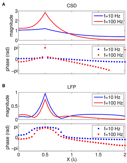
Figure A1. Theoretical CSD and LFP Green’s functions for a population of parallel finite cables. The theoretical CSD (A) and the corresponding LFP (B) laminar profiles for the population of parallel finite cables having a membrane time constant τm = 30 μm and dimensionless electrotonic length L = 2 in response to the point input currents applied at x = 0.5. The magnitude of the CSD only shows the return currents, whereas the input CSD is given by the delta function (not shown). The LFP profiles along the cylindrical column axis are found using Eq. A7 assuming a dimensionless column diameter D = 0.5. The magnitude of both CSD and the LFP are normalized to the peak value at the steady-state.
Current-Dipole Moment and Equivalent Current-Dipole Length on a Spectral Basis
The current-dipole moment P(t) = ∈tVC(r,t)rdV of a distribution of time-varying currents within the volume V when Fourier transformed, i.e.,  yields the current-dipole moment in response to sinusoidal currents oscillating at frequency f. The cylindrical volume of unit cross-section and dimensionless length L containing current sources homogeneously distributed in a plane perpendicular to the cylinder axis but varying along the axis itself will evoke the current-dipole moment
Applying Eq. A21, the current-dipole moment takes the form
The current-dipole moment in response to the input current of magnitude I0 per unit cylindrical cross-section applied at the position X′ equals to
The same current-dipole moment will result from the two point current sources of magnitude I0 and opposite polarity separated by the distance
and has a meaning of equivalent current-dipole length. Consequently, the current-dipole moment produced in response to an arbitrary distribution of input CSD  can be expressed as
being the sum of equivalent current-dipole lengths weighted by the magnitude of input CSD at each location along the length of the cables.
In case the current sources in the considered volume cylinder are generated by a population of parallel linear cables (see CSD Green’s Function for a Population of Parallel Finite Liner Cables in Appendix), the equivalent current-dipole length can be evaluated analytically by substituting the corresponding Green’s function given by Eq. A22 into Eq. A26, yielding

which is symmetric relative to the population center, because of the symmetry of the cables relative to their midpoint.
Keywords: extracellular potential, cortical column, local field potential, neuronal population, current source density, synaptic activity, inverse problem
Citation: Gratiy SL, Devor A, Einevoll GT and Dale AM (2011) On the estimation of population-specific synaptic currents from laminar multielectrode recordings. Front. Neuroinform. 5:32. doi: 10.3389/fninf.2011.00032
Received: 07 June 2011; Accepted: 21 November 2011; Published online: 20 December 2011.
Edited by:
Daniel Gardner, Weill Cornell Medical College, USACopyright: © 2011 Gratiy, Devor, Einevoll and Dale. This is an open-access article distributed under the terms of the Creative Commons Attribution Non Commercial License, which permits non-commercial use, distribution, and reproduction in other forums, provided the original authors and source are credited.
*Correspondence: Sergey L. Gratiy, Multimodal Imaging Lab, Department of Radiology, University of California San Diego, 8950 La Jolla Village Drive, La Jolla, CA 92037, USA. e-mail: sgratiy@ucsd.edu