A mutual information approach to automate identification of neuronal clusters in Drosophila brain images

1. Introduction

How the nervous system processes sensory information and generates behavior critically depends on its underlying circuitry. Mapping this circuitry (and understanding its developmental origins) is a major challenge in neuroscience, and there are currently two distinct approaches to the problem. One approach, dense reconstruction, involves labeling many neural structures in a single brain, and resolving these structures using electron microscopy (Briggman and Denk, 2006). The main difficulty with this approach is that segmenting large numbers of neural structures cannot be fully automated and is too time-intensive to perform manually (Macke et al., 2008; Jurrus et al., 2009; Seung, 2009). The second approach, sparse labeling, involves labeling few neural structures in a single brain which can be subsequently resolved using light microscopy (e.g., Otsuna and Ito, 2006; Jefferis et al., 2007; Lin et al., 2007). By imaging many sparsely labeled brains, one can piece together the neural circuitry.

One successful approach to sparse labeling has been the Mosaic Analysis with a Repressible Cell Marker (MARCM) technique in Drosophila (Lee and Luo, 1999), where only a subset of neurons that normally express a gene of interest are stochastically labeled. In MARCM, heat-shock driven mitotic recombination before cell division segregates the transcriptional repressor Gal80 from the Gal4-UAS binary transcription system. The progeny of the cell inheriting Gal80 will not display Gal4 driven expression while the progeny of the cell devoid of Gal80 will. After a recombination event, all cells displaying Gal4 driven gene expression (in this case the green fluorescent protein, GFP) are born from the same progenitor; these are referred to as a clone and in the case of neurons a neuroblast clone. If a large enough number of samples is analyzed, the stochastic nature of the recombination allows one to catalog all neurons expressing the gene in an unbiased manner.

One major bottleneck with this technique is thousands of brains may need to be imaged, and it is time consuming to manually identify the clones present in each brain. If one were able to identify the clones in a limited set of images, it would be advantageous to use this information to automatically identify clones in the remaining set of images.

The goal of this study was to develop a method to identify automatically neuroblast clones in confocal images of Drosophila brains. Our procedure is based upon the knowledge that cell bodies and their projections generated from a single clone are stereotyped across animals (Jefferis et al., 2007). We tested our procedure on 350 male Drosophila brains, where a sparse number of clones expressing the gene fruitless (fru) were stochastically labeled using MARCM and the clones present in each image were manually identified to create a training set for automatic annotation of clones in the other images. Images were filtered to accentuate the labeled cell bodies and projections (see Figure 2) and were then registered onto a common template to allow for comparison between images. Next, we compared the location of these structures, as well as the tangent vectors of the projections, across images; this allowed us to determine how informative the presence of these structures is about the presence of specific clones. Finally, by matching the parts of novel images against these informative structures, we were able to reliably determine the presence of most clones.

2. Materials and Methods

2.1. Fly Strains

fru+ Cells were labeled using the fru^GAL4 line in which the yeast transcriptional regulator Gal4 has been targeted to the start of the coding sequence for the FruM isoform (Stockinger et al., 2005). MARCM labeling used male flies of the genotype y w hs-FLP UAS-mCD8-GFP; FRT^G13UAS-mCD8-GFP/FRT^G13tubP-GAL80; fru^GAL4/ + . MARCM clones were generated by heat shocking first instar larvae for 17 minutes at 37°C between 0 and 3 h after larval hatching.

2.2. Immunochemistry

Fixation, immunochemistry, and imaging were carried out as described (Cachero et al., 2010). Primary: Mouse anti-nc82 (Wagh et al., 2006) 1:20–1:40, rat anti-CD8a (Caltag, Burlingame) 1:100, Chicken anti-GFP (Abcam, ab13970) 1:1000, rotate 2–3 days at 4°C. Secondary: Alexa-568 anti-mouse (Invitrogen) 1:200, Alexa-488 anti-rat (Invitrogen) 1:200. Rotate 2–3 days at 4°C. Prolonged incubation with both primary and secondary antibodies was required for homogeneous staining. Specimens were whole mounted in Vectashield (Vector Labs) on charged slides to avoid movement.

2.3. Image Acquisition

Confocal stacks were acquired using a Zeiss 710 confocal microscope equipped with a motorized stage which allowed unattended overnight scanning of multiple samples. Brains were scanned at 768 × 768 pixel resolution every 1 μm (0.46 μm × 0.46 μm × 1 μm) using an EC Plan-Neofluar 40×/1.30 Oil DIC M27 objective and 0.6 zoom factor. All images were taken using 16 bit color depths. To speed up processing time, all images were down-sampled by a factor of 4 × 4 × 2 and converted to 8 bit color depth for this analysis. We found that processing images at higher resolutions did not improve our algorithm’s ability to identify clones (data not shown).

2.4. Image Registration

We used nc82 neuropil staining from multichannel confocal stacks as the input to a fully automatic intensity-based (landmark free) 3D image registration software (Rohlfing and Maurer, 2003; Jefferis et al., 2007). An initial linear registration with 9 degrees of freedom (translation, rotation and scaling of each axis) was followed by a non-rigid registration that allows different brain regions to move somewhat independently, subject to a smoothness penalty (Rueckert et al., 1999). The underlying deformation model is based on third order B splines; for the central brain the final grid of B spline control points was 51 × 51 × 35, for a total of 91035 control points and therefore 273105 degrees of freedom. The algorithm typically held about two thirds of the control points fixed because they contained no useful information – usually locations outside the brain. The final control point grid had a mean spacing of 5–6 μm. The registration for the nc82 channel could then be applied to other channels containing labeled neurons.

We used an updated version of the core registration software which we have made available at http://flybrain.stanford.edu along with a control script used to coordinate multiple registrations. In the later stages of the project, the core registration toolkit (CMTK) was made open source and is now available at http://www.nitrc.org/projects/cmtk. The only pre-processing of raw confocal images before registration was rotation to match the orientation of the template to the nearest 90°, followed by export in Biorad PIC format using a plugin that we have contributed to the Fiji distribution of ImageJ¹.

2.5. Clone Identification

The central brain is generated by about 180 neuroblasts (neural stem cells) per hemisphere; each produces a specific group of neurons usually consisting of only one or two morphological classes (Ito and Awasaki, 2008). Using MARCM we generated brains in which only those fru+ neurons made by one or a few neuroblasts are labeled with a membrane targeted GFP. Each fru+ clone consisted of neurons with closely apposed cell bodies in a consistent location on the surface of the brain, primary neurites following a highly stereotyped path into the neuropil and axons and dendrites targeting reproducible neuropil locations. Our dataset of 350 images contains 60 fru+ neuroblast lineages (counting all 4 mushroom body lineages as a single clone).

2.6. Image Pre-processing

The goal of image pre-processing is to improve the fluorescent signal originating from labeled cell bodies or their projections while reducing the noise from all other sources (1). The fluorescent signal from labeled cell bodies is generally quite strong, while the signal from labeled projections can vary considerably depending on their thickness and the strength of the Gal4 driver. Thus, we processed images in two different ways to accentuate either labeled cell bodies or projections. For cell bodies (Figure 1A), images were registered onto the template brain before they were masked, setting the voxel intensity inside the neuropil to zero. We then convolved the image with a volume of 2 × 2 × 2 pixels (3.28 μm × 3.28 μm × 4.26 μm), and voxels whose intensity was greater than half of the maximum intensity of the convolved image were considered part of cell bodies (all parameters are listed in Table 1).

FIGURE 1

Figure 1. Flowchart describing the different steps of the procedure (see Materials and Methods). (A) To process cell body information, images were first reformatted onto the common template brain and were then masked to eliminate any contribution from the neuropil. Images were then isotropically filtered, thresholded and those points above threshold were compared between images based on coordinate position alone. We then calculated how informative the presence of each point was of each clone, and used these values to identify clones in novel images. (B) To process neural projection information, images were first anisotropically filtered followed by calculating the cylindrical nature each region by multiplying the two lowest eigenvalues of the Hessian matrix. Images were then thresholded before a dimension reduction algorithm was applied. Those points above threshold were then reformatted onto a common template brain and were subsequently masked to eliminate the contributions of regions outside the neuropil. We then calculated the tangent vectors to the resultant one-dimensional structures by computing the moments of inertia. This was followed by comparing points between images based on position and tangent vector. As above, we then calculated the information about the presence of a clone in each point based on these matches. Clones in novel images were identified based on how they matched points in other images, and the mutual information of these points. (C) Example projections of a raw image before filtering. (D) The same image after anisotropic filtering. (E) The image after each pixel was scored based on the Hessian matrix followed by thresholding. (F) The image after the dimension reduction algorithm was applied.

TABLE 1

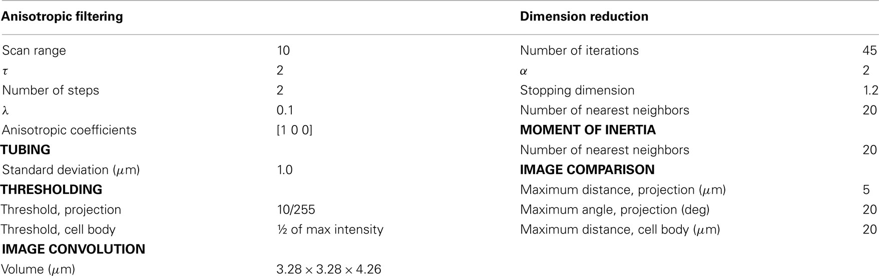
Table 1. Parameters used in the algorithms.

In order to separate signals emanating from labeled neural projections from noise (Figure 1B), we rely on the fact that neural projections are approximately cylindrical in shape. We used two complementary approaches in the pre-processing step to accentuate cylindrical structures in the image data. The first step was anisotropic diffusion filtering as described by Broser et al. (2004). As opposed to isotropic filtering which smooths the image equally in all directions, anisotropic filtering can be implemented to filter in a direction selective manner. In this implementation, the moment of inertia in a small volume surrounding each voxel is calculated to determine the local geometry (all constants used in our algorithms are presented in Table 1). Next, the image is smoothed only in the direction of the principal eigenvector of the moment of inertia. For example, if the local volume contains a cylindrical structure, the principal eigenvector would be the main axis of the cylinder and smoothing would only occur parallel to this axis. In addition to preserving cylindrical structures, the algorithm has the added advantage that it can fill in small gaps within these structures. The effect of anisotropic filtering on an example image is shown in Figures 1C,D.

To further emphasize cylindrical structures in our image, we scored how cylindrical each local region was using the ImageJ plugin “tubeness”² bundled with Fiji. The plugin works by Gaussian smoothing the image followed by multiplying the two lowest eigenvalues of the local Hessian matrix (Sato et al., 1998). High tubeness scores are given when two eigenvalues are highly negative: when the two lowest eigenvalues λ₁ and λ₂ are negative, the score is $\sqrt{{\lambda }_1{\lambda }_2},$ and is zero otherwise. The tubeness scores are then thresholded to produce a binary image. These two complementary algorithms strongly emphasized neural processes of cylindrical shape provided their diameter was not too small. The effect of the tubeness function on our example image is shown in Figure 1E. Next, there exists an optional step that removes voxels that are above threshold which form isolated regions. Specifically, one could determine the connected regions formed by the voxels above threshold (using the Matlab function bwlabeln, part of the Image Processing Toolbox), and regions consisting of less than 200 voxels were eliminated. The source code we have made available (see below) only performs this step if the user has access to the bwlabeln function. The results in this study were produced without this step. Finally, voxels above threshold were reformatted onto the common reference brain and then masked to remove voxels outside the neuropil.

2.7. Dimension Reduction

The anisotropic filtering along with the tubeness function strongly emphasized cylindrical structures, however there still existed variability in the size and shape of these structures (Figure 2). Since we wished to compare projections in different regions based on their coordinate position and their tangent vector, we applied one final algorithm to ensure that the images were mostly composed of one-dimensional structures. Condensing a three-dimensional image onto a one-dimensional structure is inherently a form of dimension reduction, and so we adapted an existing dimension reduction algorithm developed by Chigirev and Bialek (2004). The algorithm is based on the information bottleneck method (Tishby et al., 1999), which is a trade-off between minimizing the distance D and the mutual information I between the original image and its representation. Let x_i represent the coordinates of our image that are above threshold; we wish to project these onto an equal number of points, whose coordinates are given by γ_j, that form a one-dimensional representation of the original image. Letting p(γ_j| x_i) be the probability that the coordinate x_i is projected onto γ_j, and using the Euclidean distance, the functional to be minimized is:

FIGURE 2

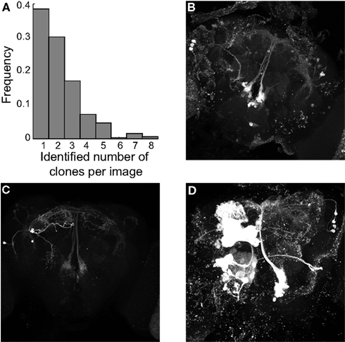
Figure 2. Example images from the dataset. (A) Histogram of the number of identified images per clone. (B) Z-projection of image SAHM16, which contained one identified clone and several unidentified. (C) Z-projection of image SAKW1 which contained two identified clones. (D) Z-projection of image SAJV25 which contained five identified clones.

$\begin{array}{lll}F& =D+\alpha I,\hfill & \\ \hfill D& =\sum _i\sum _{j}p\left(x_i\right)p\left({\gamma }_j|x_i\right){∥x_i-{\gamma }_j∥}^2\\ \hfill I& =\sum _i\sum _{j}p\left(x_i\right)p\left({\gamma }_j|x_i\right)log\frac{p\left({\gamma }_j|x_i\right)}{p\left({\gamma }_j\right)}\end{array}$

Minimizing the functional F with respect to γ and p(γ|x) leads to a set of self consistent equations which can be iteratively solved. By assigning equal probability to the N points in the image, p(x_i) = 1/N, the iteration scheme reads

$\begin{array}{ll}\hfill p\left({\gamma }_j\right)& =\frac{1}{N}\sum _{i=1}^{N}p\left({\gamma }_j|x_i\right),\hfill \\ \hfill {\gamma }_j& =\frac{1}{Np\left({\gamma }_j\right)}\sum _{i=1}^N{x}_{i}p\left({\gamma }_j|x_i\right),\hfill \\ \hfill Z\left(x_i\right)& =\sum _{j=1}^{N}p\left({\gamma }_j\right)exp\left(-\frac{1}{\alpha }{∥x_i-{\gamma }_j∥}^2\right),\hfill \\ \hfill p\left({\gamma }_j|x_i\right)& =\frac{p\left({\gamma }_j\right)}{Z\left(x_i\right)}exp\left(-\frac{1}{\alpha }{∥x_i-{\gamma }_j∥}^2\right).\hfill \end{array}$

We note that the expression for the probability p(γ_j|x_i) that the point x_i is projected onto γ_j naturally falls out of the minimization.

If we let α = 0 so that there is no mutual information constraint, the projected coordinates γ will be identical to the original coordinates x, and by default the dimensionality of the representation will be equal to the dimensionality of the original image. At the other extreme, as α becomes very large, all coordinates γ_j will collapse to a single point located at the center of mass of the image, forming a 0-dimensional representation. By using an intermediate value for α, we can force the representation to assume a one-dimensional representation. The difficulty is that different values of α are required to project the image onto a one-dimensional structure depending on the local structure of the image. In theory, one could use a variable α adapted to different portions of image. We chose a simpler approach, and chose a uniform value of α = 2, sufficiently large for most image structures, and then fixed the location of coordinates γ_j whenever their dimensionality came sufficiently close to one. Specifically, after each iteration of the algorithm we calculated the local dimensionality around each point γ_j using the Grassberger-Procaccia algorithm (Grassberger and Procaccia, 1983). Using the 20 nearest neighbors for each point, we first measured the function C(r), the number of nearest neighbors that were within a radius r of the point. The dimension is then given by

$dim=\frac{dlogC\left(r\right)}{dr}$

We considered the point γ_j belonged to a sufficiently one-dimensional structure if its local dimension was below 1.2, and we fixed its position as long as it remained below this value. This procedure was able to reduce most image structures to one-dimensional structures (Figure 1F), allowing us to easily calculate the tangent vectors for each point γ_j as described below.

2.8. Comparing Points between Images

Since neuroblast clones produce mostly stereotyped cell bodies and projections across different brains, we wished to determine whether an image contained a structure that was repeated in other images. We determined whether cell bodies and projections were repeated across images in two different manners. Points belonging to cell bodies in different images, which have been registered onto the template brain, were considered a match if they were separated by no more than 20 μm. To compare points belonging to projections between images, the local information along these one-dimensional curves can be captured by its coordinate position and its tangent vector. We again used the local moment of inertia to determine the tangent vector: for each point in a neural projection, we used its 20 nearest neighbors to compute the moment of inertia, and used the principal eigenvector as the tangent vector. Points in two different images were deemed to match if they were separated by less than 5 μm, and their tangent vectors differed by no more than 20°.

We used this procedure to separately describe each point belonging to either a cell body or a projection as a binary vector whose length matched the number of images. Each entry in the vector was associated with an image, and its value was one if that point matched a point in another image, and zero otherwise.

2.9. Calculating the Information of Each Point

Assigning binary vectors to each point belonging to a cell body or projection allowed us to determine whether the point was associated with a specific clone. Intuitively, a point would be informative of a specific clone if it matched points in images also containing the clone, but did not match points in images that did not. To quantify this measure, for each point in each image we calculated the mutual information between the images that contained a matching point and whether these images contained the clone. This was calculated separately for points belonging to cell bodies or projections. Specifically, for each image, its points, and all clones, the mutual information is:

$MI\left(\text{image,}\text{point,}\text{clone}\right)=\sum _{m=0,1}\sum _{c=0,1}p\left(c,m\right)log\frac{p\left(c,m\right)}{p\left(c\right)p\left(m\right)}$

where p(c) is the probability that an image contains the clone and p(m) is the probability that there exists a matching point. Intuitively, the mutual information between two variables measures how much our uncertainty about one variable decreases given the value of the second. Describing each point as a binary vector allows us to quickly calculate the mutual information, a necessity given that there exists thousands of points per image, 350 images, and 60 clones.

2.10. Classifying New Images

Two sets of values are needed to determine which clones are present in a new image. First, one must determine the points in all existing images that match a point in the test image. Secondly, one requires the mutual information scores for all clones. When testing whether the image contains a specific clone, the images already known to contain this clone form our template, and the score is based on the mutual information of the points in the template images that match a point in the new image. Specifically, let I_j,k= 1 if point j from the template image k matches a point in the new image and equals zero otherwise. Give this, the score of our new image for a specific clone is

$s\left(\text{imag}{\text{e}}_{\text{test}}\text{,}\text{clone}\right)=\frac{{\sum }_k{\sum }_j{I}_{j,k}max\left(0,MI\left(k,j,\text{clone}\right)-\lambda \right)}{{\sum }_k{\sum }_{j}max\left(0,MI\left(k,j,\text{clone}\right)-\lambda \right)}$

This value was calculated separately for cell bodies and for projections. For each clone, we tested 40 different values of λ, ranging in equal steps from 0.0025 to 0.1. The value that maximized the receiver operator characteristic score (see below) was used.

2.11. Scores Using the Receiver Operator Characteristic

We measured the performance of our classification using the area under the receiver operating characteristic (AROC) curve (Green and Swets, 1975). Given two random samples drawn from two distributions, the AROC measures the probability that one can correctly determine from which distribution each random sample was drawn, based on which sample has a greater value. In other words, it is a measure of how separate two distributions are from each other. Specifically, given two distributions, p(x) and q(x), the AROC is

$AROC={\int }_0^{\infty }{\int }_x^{\infty }p\left(x\right)q\left(y\right)dydx.$

In our analysis, the distribution q(y) corresponds to the distribution of scores of images containing the clone of interest, and the distribution p(x) corresponds to the distribution of scores of images not containing the clone of interest. We used this method to assess the reliability of our procedure to identify clones based on either the cell body or neural projection information. We also assessed the reliability of identifying clones by combining cell body and projection scores:

$\begin{array}{rc}\hfill p\left(x\right)& =w_{CB}{p}_{CB}\left(x\right)+w_P{p}_P\left(x\right),\hfill \\ \hfill q\left(x\right)& =w_{CB}{q}_{CB}\left(x\right)+w_P{q}_P\left(x\right),\hfill \end{array}$

where CB and P denote cell body and projection, respectively. We desired that the weights satisfy three conditions: (1) they sum to one, (2) they are monotonically increasing with respect to the AROC score, and (3) if the AROC score of a feature is close to 1, then its weight is strongly favored over the other. Several possibilities were explored before settling on the following equations that were both intuitive and produced high AROC scores:

$\begin{array}{l}{w}_{CB}=\frac{\frac{1}{1-ARO{C}_{CB}}-2}{\frac{1}{1-ARO{C}_{CB}}+\frac{1}{1-ARO{C}_P}-4},\\ w_P=\frac{\frac{1}{1-ARO{C}_P}-2}{\frac{1}{1-ARO{C}_{CB}}+\frac{1}{1-ARO{C}_P}-4}.\end{array}$

We subtracted by 2 in the numerator so that the weight was assigned a value of 0 if the corresponding AROC score was equal to 0.5 (i.e., the neural feature provided no information regarding the presence of the clone).

2.12. Computer Code and Data

The image processing pipeline and analysis code were both implemented in Matlab³. The image processing pipeline, which has external dependencies on fiji and CMTK as noted above, can also run in Octave, a free and open source alternative to Matlab⁴. This allowed us to carry out some investigations of different parameters using a Linux/Sun Grid Engine based compute cluster. However all regular image processing and all analysis was carried out on MacOSX or Windows desktop machines. Full source code is available for download at https://github.com/jefferis/FruCloneClustering. A simple installation script is provided. Functions are documented and some examples of their use are provided. The final processed data used to generate the figures in this manuscript is available for immediate web download via the installation script, along with some of the original image data. Further details of these supplemental data are presented at http://jefferislab.org/data and the full image dataset is available on request from GSXEJ on a hard drive.

3. Results

We used cross-validation to test our procedure on a set of 350 images of male Drosophila brains. Only clones that were present in at least 4 brains were included in the analysis, giving a total of 60 clones. Images contained from one to eight identified clones with a median of two (Figure 2A). Three example images with various levels of background noise are shown in Figures 2B–D containing one, two, and five identified clones, respectively. It is important to note that the number of identified clones per images does not fully capture the number of structures in each image. For example, the image shown in Figure 2B contains only one identified clone, but also contains an optic lobe clone (which we did not seek to identify) as well as two additional clones that were only weakly labeled and thus considered part of the background. We believe that a single metric such as the number of identified clones per image does not fully convey the complexity of the dataset and the reader is encouraged to examine the sample images from the first three clones available for download (see Materials and Methods) to form their own opinion.

To determine whether an image contained a certain clone, we compared it against a template derived from all the images in our dataset containing that specific clone (however the image we were testing was never included in any template). In Figure 3A, we show a test image (black points, same brain as presented in Figure 1) containing an AL-PN clone compared against one of the 47 AL-PN template images (red points) and one of the 7 mcAL-PN template images (blue points) where the brightness of each red and blue point corresponds to its mutual information. Our algorithm finds the points in each template image that match at least one point in the test image; in this case, more points from the AL-PN template image matched points in the test image compared to the mcAL-PN template image (Figure 3B). Thus, this AL-PN template image received a greater score (which depends on the proportion of matching points and their mutual information, see Materials and Methods) for this test image compared to the mcAL-PN template image.

FIGURE 3

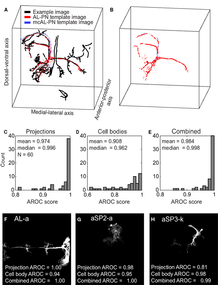
Figure 3. Assessment of the clone identification algorithm using cross-validation. (A) A processed test image (black points) containing an AL-PN clone is compared against a AL-PN template image (red points) and a mcAL-PN template image (blue points). The brightness of the red and blue points correspond to the mutual information of the point. (B) Same as (A), except only those points from the two template images that matched a point in the test image are shown.(C) Distribution of projection AROC scores for the 60 clones. (D) Same as (C), except showing the cell body AROC scores. (E) Same as (C), except showing the combined AROC score. (F–H) Z-projections of three example clones with variable projection and cell body AROC scores.

In total, 350 images were compared against 60 clone templates. For each clone, we divided the scores for all 350 images into two distributions: one distribution for images that contained the clone and one for images that did not. A template can reliably identify a specific clone if there exists little overlap between the two distributions. We quantified the separation between the distributions using the area under the ROC curve (AROC, see Materials and Methods). Given a random sample from each of these two distributions, the AROC gives the probability that the sample image containing the clone scores higher than the sample image without the clone. A score of 0.5 indicates that one can only guess at chance whether the image contained the clone while a score of 1 indicates that one can always determine whether the image contained the clone.

Overall, we could reliably identify clones using templates based on either neural projections or cell bodies (mean projection AROC = 0.974, median = 0.996; mean cell body AROC = 0.908, median = 0.962) although both the mean and median AROC scores were greater for templates based on neural projections (p < 10⁻³, two-sided t-test; p < 10⁻⁵, two-sided Wilcoxon signed-rank test; Figures 3C,D). We could improve upon our ability to identify clones by combining the projection and cell body scores (see Materials and Methods); mean combined AROC scores were greater than mean projection scores (mean combined AROC = 0.984, p = 0.041, two-sided t-test), although the increase in the median combined AROC score was not significant (median combined AROC = 0.998, p = 0.096, two-sided Wilcoxon signed-rank test; Figure 3E). Although our method was capable of reliably identifying the majority of clones (combined AROC scores for 40 clones were above 0.99), certain clones proved more difficult to identify (scores for 3 clones below 0.9). We wished to understand the source of this variability.

Interestingly, the number of clones per image was not correlated with the combined AROC scores (Spearman correlation coefficient; r = −0.16, p = 0.23). The two clones with the greatest number of images, the mushroom body (78 images) and AL-PNs (48 images) clones scored lower than the average (projection AROC scores of 0.932 and 0.930, respectively). For these clones, more than one projection pattern existed, reducing the amount of common processes shared by all images containing the clone.

One problem that our algorithm encountered was the variable level of fruitless driven GFP expression. In clones mcAL-b and aSP3-i, strong fru expression allowed Gal4 to circumvent the Gal80 repressor, leading to low-level “leak” of GFP expression independent of any labeling event. A clone was only considered labeled if it strongly expressed GFP in an image, but in many cases, our algorithm was able to detect the low expression levels of these clones that were present in many images. Calculating the mutual information for these clones and scoring them was troublesome since they were often present in images where their presence had not been manually annotated. This partially explains why clones mcAL-b and aSP3-i had projection AROC scores of 0.904 and 0.972, respectively, well below the median score.

Another contributing factor was the amount of overlap between different clones: clones located in unique regions in the brain were much easier to identify than those clones that overlapped substantially with others. For example, the clone AL-a (Figure 3F) which had a perfect projection AROC score of 1.0, had a distinctive projection that crosses both hemispheres of the brain. Even clones that did not possess such a well defined main neurite, such as the clone aSP2-a with a projection AROC score of 0.983 (Figure 3G), could be identified due to its unique projection. On the other hand, clones such as aSP3-k (projection AROC score of 0.811; Figure 3H) were located in densely populated areas of the brain, overlapping considerably with other clones. For several clones with lower projection AROC, combining the cell body scores led to a significant improvement in their identification. For example, the combined AROC score for clone aSP3-k was 0.986, an increase of 0.155 compared to its projection AROC score.

In this dataset, there was a large variety in the number of images per clone, ranging from 4 to 78 (median 9.5). Much time could be saved if one had to identify only a few examples of each clone and use this procedure to automatically identify clones in the remaining images. We wondered whether clone templates consisting of small numbers of example images could be used to reliably identify clones in novel images. Thus, we repeated the cross-validation analysis used for 3, but we used a maximum of either three, four, or five images per clone to determine the mutual information and classify new images (Figure 4). If a clone had more than the maximum number of images, we selected the image names ranked first alphabetically.

FIGURE 4

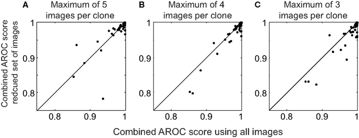
Figure 4. Performance using a limited set of images in the clone templates. (A) Scatter plot of the combined AROC scores using a maximum of five images per clone template compared to the combined AROC scores using all images. (B,C) Same as (A), except using a maximum of 4 and 3 images to form the templates, respectively.

Limiting the number of images in the template had a surprisingly small effect on the AROC scores. The median combined AROC scores were 0.997, 0.996, and 0.993 using a maximum of 5, 4, and 3 images, respectively (Figure 4). Scores for several images actually increased when using a reduced set of images, highlighting the fact that including poor quality images can degrade the clone template, and that choosing a small number of high quality images per clone can be sufficient to reliably identify novel images. Thus, our algorithm can reliably identify clones using a relatively small number of images to form the templates.

In our procedure, a decision on whether an image contains a clone ultimately depends on how the image scored compared to a user-determined threshold. As an additional test, we considered a different metric of success. We selected the 135 images in our dataset that, according to our original annotation, contained a single clone. We compared these images against all 60 clone templates and measured whether the clone template with the highest score matched the clone contained in the image. Of 135 images, 125 scored highest against the matching clone template. For five of the images that failed, our algorithm identified either mcAL-b or aSP3-i, two clones that showed GFP expression independent of MARCM labeling events (see above). Our algorithm correctly detected the presence of these neurons although the images were not annotated as possessing either clone. For the other five images our algorithm failed to identify the correct clone.

All of the analysis that we have presented so far has examined images from the same dataset used to generate the classifier. These images are challenging because they contain complex labeling patterns with multiple neuronal clusters and a significant amount of image noise; furthermore all testing was done by leave-one-out cross-validation, so no image could contribute information to the classifier used for its identification. Nevertheless, these confocal image data were acquired in a single lab with quite consistent experimental conditions. We therefore decided to test the generality and robustness of our approach by using rather different input data. In parallel with our own group’s studies of the neuroanatomy of the fruitless courtship circuit, Yu et al. (2010) used image registration (to their own distinct template brain) combined with a distinct genetic labeling strategy to divide fruitless expressing neurons into about 110 genetically and morphologically discrete clusters. As part of their data analysis Yu et al. (2010) traced the main processes of many of these neuronal groups, resulting in simple neuronal skeletons with only a few branches. Since Cachero et al. (2010) and Yu et al. (2010) were in theory studying exactly the same population of fruitless expressing neurons it should be a relatively simple matter to identify the corresponding neuronal clusters from both studies. However in practice, we have found that this is challenging even for expert neuroanatomists (AO, SC, GSXEJ, unpublished observations). We therefore decided to use the neuronal tracings from Yu et al. (2010) to search the image classifier developed in this study from the image data of Cachero et al. (2010).

For searching, the tracings were first transformed onto the IS2 template brain used in this study. Their 3D coordinates were then extracted (ignoring connectivity) and tangent vectors and local dimensionality were calculated in identical fashion to the approach used to characterize neuronal projections from images in the main dataset. The mutual information score against each template clone was then calculated using the same procedure described in 2. We found numerous cases where the top hit for the tracings differed from our tentative manual annotation. Figure 5 presents two such examples. In the first case (Figure 5A) one cluster (aDT3) of olfactory projection neurons defined by Yu et al. (2010) mapped onto two neuroblast clusters according to Cachero et al. (2010). The mutual information approach successfully identified the correct neuroblast clone corresponding to the query tracing (mAL-PNs), which had been incorrectly matched with the second neuroblast cluster (AL-PNs) during manual annotation. As a second example, no candidate had been proposed for the aSP7 cluster of Yu et al. (2010) during manual annotation. However searching with a query tracing against the 60 clone templates identified a strong and unique match in clone AL-b (Figure 5B). Three dimensional volume rendering of an AL-b clone and the tracing provided a visual confirmation of the match (Figure 5C).

FIGURE 5

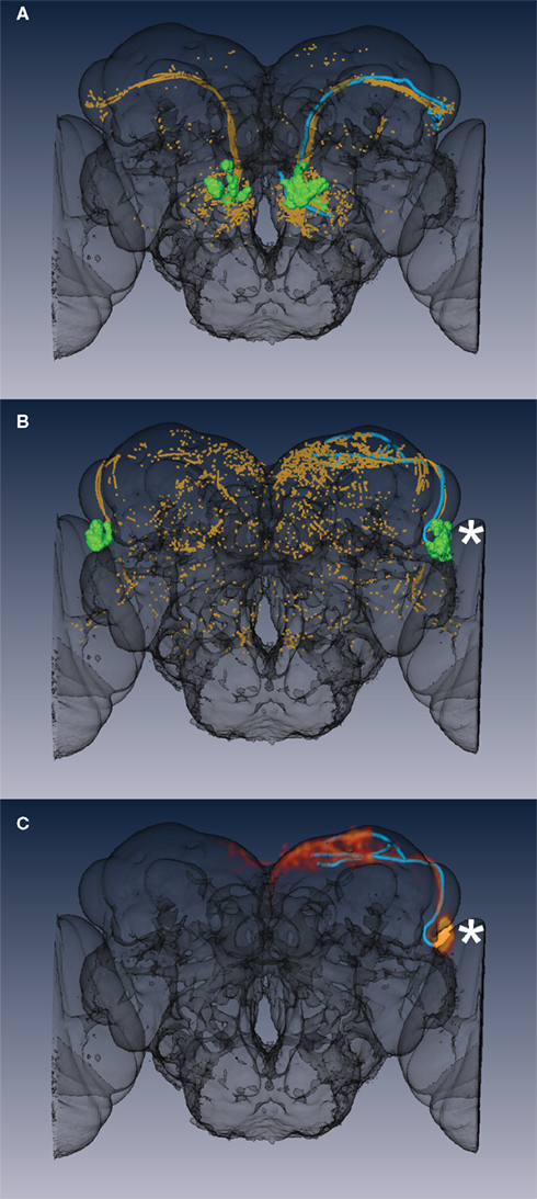
Figure 5. Searching fruitless clone templates using partial tracings. (A) A query tracing (cyan, aDT3 cluster) was used to search the classifier developed in this study. The informative (high mutual information) points from the closest matching template clone are shown in orange, while the cell bodies are shown in green. (B) A similar search was carried out for a second tracing (aSP7 cluster). (C) Volume rendering of an image containing the AL-b neuroblast clone (red/orange) showing the excellent match with the query tracing (cyan). Notice also the excellent correspondence of the position of the cell body cluster (asterisk) with the green template cell bodies in (B). In both (A,B) informative points (orange) are present on both sides of the brain since the training set has clones in the left and right hemispheres (see Materials and Methods for details of this issue).

4. Discussion

In this study, we have described how one can speed up the identification of Drosophila neuroblast clones in large datasets. By manually identifying clones in a small set of images, our procedure identifies informative regions in the brain, allowing one to detect the presence of clones in novel images. Crucially, one must identify only a handful of images for most clones (Figure 4) before using this method to identify clones in novel images.

Overall, our procedure was successful at reliably identifying the majority of clones; the combined AROC scores for 40 out of 60 clones were above 0.99 while 48 clones scored above 0.98 (Figure 3E). However, our procedure had difficulty detecting several clones for reasons outlined in the Results. Some of these difficulties were not related to our procedure, but can be attributed to the annotation of our dataset which was not designed for this study. For example, AL-PN and mushroom body clones both contain several different projection patterns; labeling these distinct projection patterns as different clone types could improve the chances of successful identification.

Another problem unrelated to our procedure was the low-level leaky expression of GFP in neurons from two of the clones. In many images the weak fluorescence from these clones was detected even though the image were annotated as not containing the clone. In future implementations it might be helpful to raise the threshold in the regions of the brain where these clones are located to prevent the false detection of low-level GFP leak. In contrast, GFP expression for some clones was always weak; in these cases, one could lower the threshold in the brain regions where these clones are located to guarantee that their presence is detected.

As seen in Figure 4, reducing the number of images per clone had a marginal effect on performance, and in some cases actually improved reliability. One possible improvement to our procedure would be to optimally select images used to form the templates; one can visually identify images of poor quality that would degrade the quality of the template. A more rigorous approach would be to select a subset of images that maximizes the mutual information for the most informative points. For the majority of clones with AROC scores close to 1.0 this would probably have little effect, but may prove beneficial for the lower scoring clones.

For many clones, the main neurite was relatively small compared to the diffuse projections that were too small to resolve in the confocal data. Our filtering approach for neural projections was meant to accentuate cylindrical structures, such as the main neurites and was not designed for these finer, more diffuse structures. As a result the filtered output of diffuse projections did not resemble the original image. One possible modification would be to employ a second, separate filter adapted to accentuate these diffuse projections. One could then try to identify diffuse projections that are stereotyped across animals. Another possible modification to our pre-processing methods could be to improve how we process images to identify cell bodies. The combination of a mask to exclude the neuropil with a simple convolution worked well for our dataset. However for other datasets where cell bodies are not so readily identifiable based on position or so cleanly separated from image noise, 3D versions of more advanced algorithms may be required (e.g., Huang et al., 2010; Wu et al., 2010).

Although this procedure relies on manually identifying clones for an initial set of images, it is possible to adapt this method to identify clones without any prior annotation. As described in 2, every point in every image is assigned a binary vector with length equal to the number of images in the dataset. Each entry in the vector indicates whether the point matches a point in a different image. Clustering algorithms (Slonim et al., 2005) can then be employed to find those points that have matches in a common set of images. Using this approach, we found that many clusters were associated with specific clones (results not shown), however, many clusters were comprised of points belonging to several overlapping clones. Provided that one could properly separate clusters associated with a single clone, manual annotation of the dataset might no longer be necessary. Furthermore such unsupervised learning could also be used to bootstrap a supervised learning process: unsupervised clusters could be manually validated and then used as the basis for learned categories.

Large scale efforts to map the fly brain are resulting in a variety of single cell and neuronal cluster level data (Cachero et al., 2010; Yu et al., 2010; Chiang et al., 2011; Peng et al., 2011). There is therefore a pressing need to develop approaches that can integrate neuroanatomical data across different labeling approaches and laboratories. We have demonstrated that our approach can be used for neuronal matching of tracings of image data obtained in a second laboratory that encompass only fragments of a full neuronal cluster. Although a quantitative study of this application is beyond the scope of the current work, we believe that our approach is sufficiently robust and general that it could be of widespread use in this area. Furthermore, the same strategy could be adapted for matching long range, projectome level data from mouse (Bohland et al., 2009) or human brains (Hagmann et al., 2008), since the spatial location and orientation of neuronal fibers are likely to have rather similar properties to the Drosophila neuron clusters we have examined.

Conflict of Interest Statement

The authors declare that the research was conducted in the absence of any commercial or financial relationships that could be construed as a potential conflict of interest.

Acknowledgments

We thank members of the Jefferis lab for comments on the manuscript, Jake Grimmett for assistance with the LMB’s compute cluster and Steffen Prohaska and Torsten Rohlfing for discussions about image analysis and registration. This study made use of the Computational Morphometry Toolkit (http://www.nitrc.org/projects/cmtk), supported by the National Institute of Biomedical Imaging and Bioengineering. This work was supported by the Medical Research Council [MRC file reference U105188491] and a European Research Council Starting Investigator Grant (GSXEJ).

Footnotes

1. ^http://fiji.sc
2. ^http://homepages.inf.ed.ac.uk/s9808248/imagej/tubeness
3. ^http://www.mathworks.co.uk
4. ^http://www.gnu.org/software/octave/

References

Bohland, J. W., Wu, C., Barbas, H., Bokil, H., Bota, M., Breiter, H. C., Cline, H. T., Doyle, J. C., Freed, P. J., Greenspan, R. J., Haber, S. N., Hawrylycz, M., Herrera, D. G., Hilgetag, C. C., Huang, Z. J., Jones, A., Jones, E. G., Karten, H. J., Kleinfeld, D., Kötter, R., Lester, H. A., Lin, J. M., Mensh, B. D., Mikula, S., Panksepp, J., Price, J. L., Safdieh, J., Saper, C. B., Schiff, N. D., Schmahmann, J. D., Stillman, B. W., Svoboda, K., Swanson, L. W., Toga, A. W., Van Essen, D. C., Watson, J. D., and Mitra, P. P. (2009). A proposal for a coordinated effort for the determination of brainwide neuroanatomical connectivity in model organisms at a mesoscopic scale. PLoS Comput. Biol. 5, e1000334. doi:10.1371/journal.pcbi.1000334

Pubmed Abstract | Pubmed Full Text | CrossRef Full Text

Briggman, K. L., and Denk, W. (2006). Towards neural circuit reconstruction with volume electron microscopy techniques. Curr. Opin. Neurobiol. 16, 562–570.

Pubmed Abstract | Pubmed Full Text | CrossRef Full Text

Broser, P. J., Schulte, R., Lang, S., Roth, A., Helmchen, F., Waters, J., Sakmann, B., and Wittum, G. (2004). Nonlinear anisotropic diffusion filtering of three-dimensional image data from two-photon microscopy. J. Biomed. Opt. 9, 1253–1264.

Pubmed Abstract | Pubmed Full Text | CrossRef Full Text

Cachero, S., Ostrovsky, A. D., Yu, J. Y., Dickson, B. J., and Jefferis, G. S. X. E. (2010). Sexual dimorphism in the fly brain. Curr. Biol. 20, 1589–1601.

Pubmed Abstract | Pubmed Full Text | CrossRef Full Text

Chiang, A.-S., Lin, C.-Y., Chuang, C.-C., Chang, H.-M., Hsieh, C.-H., Yeh, C.-W., Shih, C.-T., Wu, J.-J., Wang, G.-T., Chen, Y.-C., Wu, C.-C., Chen, G.-Y., Ching, Y.-T., Lee, P.-C., Lin, C.-Y., Lin, H.-H., Wu, C.-C., Hsu, H.-W., Huang, Y.-A., Chen, J.-Y., Chiang, H.-J., Lu, C.-F., Ni, R.-F., Yeh, C.-Y., and Hwang, J.-K. (2011). Three-dimensional reconstruction of brain-wide wiring networks in Drosophila at single-cell resolution. Curr. Biol. 21, 1–11.

Pubmed Abstract | Pubmed Full Text | CrossRef Full Text

Chigirev, D., and Bialek, W. (2004). “Optimal manifold representation of data: an information theoretic approach,” in Advances in Neural Information Processing Systems 16: Proceedings of the 2003 Conference (Cambridge: The MIT Press), 161.

Grassberger, P., and Procaccia, I. (1983). Characterization of strange attractors. Phys. Rev. Lett. 50, 346–349.

CrossRef Full Text

Green, D. M., and Swets, J. A. (1975). Signal Detection Theory and Psychophysics. Huntington, NY: Robert E. Krieger.

Hagmann, P., Cammoun, L., Gigandet, X., Meuli, R., Honey, C. J., Wedeen, V. J., and Sporns, O. (2008). Mapping the structural core of human cerebral cortex. PLoS Biol. 6, e159. doi:10.1371/journal.pbio.0060159

CrossRef Full Text

Huang, Y., Zhou, X., Miao, B., Lipinski, M., Zhang, Y., Li, F., Degterev, A., Yuan, J., Hu, G., and Wong, S. T. C. (2010). A computational framework for studying neuron morphology from in vitro high content neuron-based screening. J. Neurosci. Methods 190, 299–309.

Pubmed Abstract | Pubmed Full Text | CrossRef Full Text

Ito, K., and Awasaki, T. (2008). Clonal unit architecture of the adult fly brain. Adv. Exp. Med. Biol. 628, 137–158.

Pubmed Abstract | Pubmed Full Text | CrossRef Full Text

Jefferis, G. S. X. E., Potter, C. J., Chan, A. M., Marin, E. C., Rohlfing, T., Maurer, C. R. J., and Luo, L. (2007). Comprehensive maps of Drosophila higher olfactory centers: spatially segregated fruit and pheromone representation. Cell 128, 1187–1203.

Pubmed Abstract | Pubmed Full Text | CrossRef Full Text

Jurrus, E., Hardy, M., Tasdizen, T., Fletcher, P. T., Koshevoy, P., Chien, C.-B., Denk, W., and Whitaker, R. (2009). Axon tracking in serial block-face scanning electron microscopy. Med. Image Anal. 13, 180–188.

Pubmed Abstract | Pubmed Full Text | CrossRef Full Text

Lee, T., and Luo, L. (1999). Mosaic analysis with a repressible cell marker for studies of gene function in neuronal morphogenesis. Neuron 22, 451–461.

Pubmed Abstract | Pubmed Full Text | CrossRef Full Text

Lin, H.-H., Lai, J. S.-Y., Chin, A.-L., Chen, Y.-C., and Chiang, A.-S. (2007). A map of olfactory representation in the Drosophila mushroom body. Cell 128, 1205–1217.

Pubmed Abstract | Pubmed Full Text | CrossRef Full Text

Macke, J. H., Maack, N., Gupta, R., Denk, W., Scholkopf, B., and Borst, A. (2008). Contour-propagation algorithms for semi-automated reconstruction of neural processes. J. Neurosci. Methods 167, 349–357.

Pubmed Abstract | Pubmed Full Text | CrossRef Full Text

Otsuna, H., and Ito, K. (2006). Systematic analysis of the visual projection neurons of Drosophila melanogaster. I. Lobula-specific pathways. J. Comp. Neurol. 497, 928–958.

Pubmed Abstract | Pubmed Full Text | CrossRef Full Text

Peng, H., Chung, P., Long, F., Qu, L., Jenett, A., Seeds, A. M., Myers, E. W., and Simpson, J. H. (2011). Brainaligner: 3d registration atlases of Drosophila brains. Nat. Methods 8, 493–500.

Pubmed Abstract | Pubmed Full Text | CrossRef Full Text

Rohlfing, T., and Maurer, C. R. J. (2003). Nonrigid image registration in shared-memory multiprocessor environments with application to brains, breasts, and bees. IEEE Trans. Inf. Technol. Biomed. 7, 16–25.

Pubmed Abstract | Pubmed Full Text | CrossRef Full Text

Rueckert, D., Sonoda, L. I., Hayes, C., Hill, D. L., Leach, M. O., and Hawkes, D. J. (1999). Nonrigid registration using free-form deformations: application to breast mr images. IEEE Trans. Med. Imaging 18, 712–721.

Pubmed Abstract | Pubmed Full Text | CrossRef Full Text

Sato, Y., Nakajima, S., Shiraga, N., Atsumi, H., Yoshida, S., Koller, T., Gerig, G., and Kikinis, R. (1998). Three-dimensional multi-scale line filter for segmentation and visualization of curvilinear structures in medical images. Med. Image Anal. 2, 143–168.

Pubmed Abstract | Pubmed Full Text | CrossRef Full Text

Seung, H. S. (2009). Reading the book of memory: sparse sampling versus dense mapping of connectomes. Neuron 62, 17–29.

Pubmed Abstract | Pubmed Full Text | CrossRef Full Text

Slonim, N., Atwal, G., Tkacik, G., and Bialek, W. (2005). Information-based clustering. Proc. Natl. Acad. Sci. U.S.A. 102, 18297.

Pubmed Abstract | Pubmed Full Text | CrossRef Full Text

Stockinger, P., Kvitsiani, D., Rotkopf, S., Tirian, L., and Dickson, B. J. (2005). Neural circuitry that governs Drosophila male courtship behavior. Cell 121, 795–807.

Pubmed Abstract | Pubmed Full Text | CrossRef Full Text

Tishby, N., Pereira, F., and Bialek, W. (1999). “The information bottleneck method,” in Proceedings of the 37th Allerton Conference on Communication, Control, and Computing, eds B. Hajek, and R. S. Sreenivas (Urbana: University of Illinois Press).

Wagh, D. A., Rasse, T. M., Asan, E., Hofbauer, A., Schwenkert, I., Durrbeck, H., Buchner, S., Dabauvalle, M. C., Schmidt, M., Qin, G., Wichmann, C., Kittel, R., Sigrist, S. J., and Buchner, E. (2006). Bruchpilot, a protein with homology to elks/cast, is required for structural integrity and function of synaptic active zones in Drosophila. Neuron 49, 833–844.

Pubmed Abstract | Pubmed Full Text | CrossRef Full Text

Wu, C., Schulte, J., Sepp, K. J., Littleton, J. T., and Hong, P. (2010). Automatic robust neurite detection and morphological analysis of neuronal cell cultures in high-content screening. Neuroinformatics 8, 83–100.

Pubmed Abstract | Pubmed Full Text | CrossRef Full Text

Yu, J. Y., Kanai, M. I., Demir, E., Jefferis, G. S. X. E., and Dickson, B. J. (2010). Cellular organization of the neural circuit that drives Drosophila courtship behavior. Curr. Biol. 20, 1602–1614.

Pubmed Abstract | Pubmed Full Text | CrossRef Full Text