Natural selection at work: an accelerated evolutionary computing approach to predictive model selection

We implement genetic algorithm based predictive model building as an alternative to the traditional stepwise regression. We then employ the Information Complexity Measure (ICOMP) as a measure of model fitness instead of the commonly used measure of R-square. Furthermore, we propose some modifications to the genetic algorithm to increase the overall efficiency.

Introduction

Variable selection in predictive model building is known to be a difficult procedure. The main difficulty lies in determining what variables best explain the system. For instance, exhaustive search becomes unreasonable as the number of variables increases; employing a multiple regression search produces over one billion possible models for data with 30 explanatory variables.

In ecological studies, one of the commonly used methods for selection is stepwise regression, with forward or backward variable selection algorithms. These methods have been criticized for lacking the ability to truly pick the best model for several reasons (Boyce et al., 1974; Wilkinson, 1989). One problem is that the choice by which the variables enter the selection algorithm is not justified theoretically. In addition, the probabilities for the selection procedure are chosen arbitrarily, which may lead to a poorly selected model. Since these methods employ local search, it is unlikely that the global maximum set of variables will be found (Mantel, 1970; Hocking, 1976, 1983; Moses, 1986).

We propose the use of genetic algorithms (GAs) to determine the subset of variables with the highest goodness of fit for a multiple regression model. Due to their global search capabilities, the GA based model building is not prone to the problems associated with local search method, hence is a wise choice for this procedure.

We now explain the basics of GAs briefly; a thorough one can be found in Goldberg (1989).

Genetic Algorithms

Genetic algorithms are a set of optimization techniques inspired by biological evolution, operating under natural selection. First developed by Holland (1975), they have grown in popularity because of the ability of the algorithm to perform well on many different types of problems. In a GA, possible solutions are coded using binary strings, which are called chromosomes. Each chromosome has a fitness value associated with it based on how well the string model parameters predicts the dependent variables. During each generation, which is the time step of the algorithm, a population of chromosomes compete to have their “genes” passed on to the next generation. The selection step is used to pick the chromosomes for the next generation based on their fitness. Those selected enter the mating pool, where two chromosomes mate using crossover. During this phase, parts of each parent string are swapped to form two new chromosomes that have certain aspects of their parents. After crossover, mutation is implemented. Mutation occurs with a small probability and is defined by a change from 0 to 1 or 1 to 0 in the binary string. Mutation allows the introduction of new “genes” that were either lost from the population or were not there to start with. Through successive generations, increasingly better chromosomes come to dominate the population, and the optimal solution (or something very close) is realized.

Complexity of a Model

A key component of a GA is the method to evaluate the fitness of a chromosome. Thus, in order to use a GA for model selection in multiple regression, a way to evaluate the chromosomes is needed. More specifically the fittest chromosome is the set of parameters that maximizes the explanatory power of the model with minimum number of parameters. Bozdogan (1988, 2004) considered “complexity” as a measure of fitness, which can be described as follows:

The complexity of a system (of any type) is a measure of the degree of interdependency between the whole system and a simple enumerative composition of its subsystems or parts.

The concept of “information complexity” was first introduced by Akaike (1973) as a measure of the complexity of a model: it is a relative measure of the information lost when a given model is used, and can be described as a function of the precision and accuracy of the model. The expression for AIC is given as

where denotes the maximum likelihood function, is the maximum likelihood estimate of parameter vector θ_k, and m(k) is the number of parameters in the model. The first term of AIC gives the lack of fit of the model, and the second term is a penalty for the number of parameters in the model. The model with the lowest AIC value is considered the best, because the model successfully determines the underlying stochastic process with the least number of parameters. Although AIC does take into account the problem of over-fitting, where other measures such as R-square do not, AIC is not sensitive to parameter dependency, which is an important component for model selection. If a model with both low variance and low covariance can be produced, then the parameters can be better estimated, as they will not be correlated. As an alternative to AIC, we consider ICOMP as a complexity measure which considers variance and covariance, and accounts for the problem of over-fitting the model. It is calculated by

where again denotes the maximum likelihood function, is the maximum likelihood estimate of parameter vector θ_k under the model m_k, C is a real-valued complexity measure, and is the estimated covariance matrix of the parameters of the model. Note that the first term in AIC is double the first term in ICOMP. The main difference between the two measures of complexity is that AIC only considers the number of parameters as a penalty, whereas ICOMP considers the covariance between parameters. In predictive model building, we use ICOMP (IFIM) as our multiple regression model selection criterion. This value for ICOMP is based on the inverse-Fisher information matrix (IFIM). For multiple regression, the value of ICOMP can be directly calculated after regression is implemented, and is given by

where

n is the number of parameters in the model, q is the number of observations, is the trace of the observation matrix multiplied by its inverse and then scaled by and is the determinant of the previous matrix.

Since the model with the lowest ICOMP value is considered the best, the GA chooses strings biased toward those with the lowest value. A commonly used method to form the mating pool is “proportional selection,” which depends on selecting strings for the mating pool with a probability proportional to their fitnesses. In proportional selection, the first step of the calculation of the fitness values is subtracting the ICOMP value of each string in that generation from the maximum value of ICOMP in the population. That is,

for each i = 1,2,…,N, where N is the size of the population. Then the average ICOMP difference (the “average fitness”) for the total population is calculated as

Finally, each string is given a fitness value that is the ratio of its ICOMP difference and the average fitness of the population:

A Genetic Algorithm for Multiple Linear Regression Model Selection

Here we consider the implementation of GA’s for predictive model selection and discuss possible improvements.

Background

The first step to implementing a GA for any optimization problem is to encode the input variable into binary strings. In the case of multiple linear regression, we have q data points with n explanatory variables and one response variable. We wish to fit the data to

where y is an n × 1 response vector, X is an n × q matrix of the data points, β is a q × 1 coefficient matrix, and ε is an n × 1 error vector with entries from independent normal distributions [N(0, σ²) for all components]. The encoding is done by creating a binary string which has n + 1 bits, where each bit represents a different parameter of the model and an intercept. The last n bits correspond to the n explanatory variables contained in the dataset, whereas the first bit is the intercept for the linear model. A parameter is included in the model if the value of the bit for that parameter is a 1 and is excluded if it is a 0. For example, suppose we have a dataset where we are interested in predicting the reproductive fitness of a species of trees. The possible explanatory variables may include:

1. Age of tree,

2. Height of tree,

3. Soil pH,

4. Density of trees in the surrounding area,

5. Average temperature of environment,

6. Average rainfall of environment,

7. Circumference of trunk,

8. Longitude of environment,

9. Latitude of environment,

10. Prevalence of disease in environment.

In this case, each binary string will have 11 bits. For example, the string 10010111101 would represent a model which includes the intercept, soil pH, average temperature of environment, average rainfall of environment, circumference of trunk, longitude of environment, and prevalence of disease in environment. Similarly, the string 00001000110 is a model that has no intercept, and includes density of trees in the surrounding area, longitude of environment, and latitude of environment (see Table 1).

TABLE 1

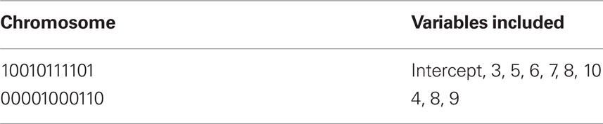
Table 1. Chromosomes and variables included by the model it represents.

The probability that a string will be chosen for the mating pool is proportional to its fitness value. Note that the string with the worst ICOMP value will never be picked for the mating pool, as its fitness will be 0.

Now that we have a method of encoding information and a method to evaluate the fitness values, we have to determine the remaining parameters of the GA. The first one we consider is the method of creating the initial population and determining its size. Unless previous knowledge about the problem is given, it is commonplace in GAs to randomly generate binary strings (Goldberg, 1989). However, in the case of model selection, a user may want to force a parameter(s) to be included, even if it is not part of the model with the lowest complexity. In this case, the initial population can be generated in such a way that certain parameters are always in the model. In addition to determining the method to generate the population, the user must choose the size of the initial population. This decision can be difficult. Generally the size should not be too large, as this will slow the algorithm, and should not be so small that genetic drift takes over the course of evolution of the population. In typical GAs, the size of the population stays the same; however, this may not be an effective use of computation. We will see in the next section that starting with a larger size then reducing it may be more effective.

Finally, we discuss the genetic operators which allow the algorithm to find the optimal model. There are two operators that are generally implemented in GAs: crossover and mutation. Crossover mimics biological crossover in a simplified manner. First, the probability of crossover, p_c, is chosen. In the mating pool, a pair of strings are chosen along with a random number from [0, 1]. If that number is less than the probability of crossover, crossover occurs. Thus, if p_c = 1, then every pair will cross, and if p_c = 0, then no strings will be altered by crossover. After the choice of p_c, the number of crossover points must be chosen. The location of the crossover points is chosen at random. Then the bits from the parent strings are swapped to create two new offspring strings (see Figure 1). The purpose of crossover is to bring together models which have components that reduce complexity. Recall the previous example about trees, where we specified two strings, which we will call Parent 1 and Parent 2. Applying crossover to the two parents creates two offspring (see Figure 1), where Offspring 1 represents a model with an intercept, soil pH, average temperature of environment, longitude of environment, latitude of environment, and prevalence of disease in environment, and Offspring 2 represents a model that includes density of trees in the surrounding area, average rainfall of environment, circumference of trunk, and longitude of environment. Through successive generations and application of crossover of low complexity models, the algorithm is able to find the least complex model (or something close to it) to explain the data.

FIGURE 1

Figure 1. Diagram of crossover with two points.

Crossover can only generate models that include parameters which already exist in the population. But, what happens if the actual least complex model includes a parameter that is not present in the population, that is, the position in the string that represents the parameter is fixed at 0? Mutation alleviates this problem. Mutation in GAs is similar to the mutation that occurs naturally in DNA. First, the probability of mutation, p_m, has to be determined. This value gives the probability that at each location in the string the bit will be flipped. Flipping is defined as a change of a 0 to 1 or a 1 to a 0. Typically, mutation rates are low, on the order of 10⁻³ to 10⁻⁵. However, strings used for other applications of GA’s are usually longer than the ones used for determining least complex models. Although there are ongoing studies on determining optimal crossover and mutation rates (such as Nested GAs, Self-adjusting parameterless GAs), these rates can be determined by trial and error or by pilot runs before the actual data set has been used to build a model.

We conclude this section with a pseudo code for a GA used to find the least complex model that sufficiently describes the data.

1. Generate Initial Population

2. While (t < Max Generations OR the maximum number of computations have not been executed)

(a) Calculate ICOMP for the model each string encodes

(b) Select strings for the mating pool

(c) Create a new population using crossover

(d) Mutate new population

(e) t = t + 1

3. End

Model Building VIA Accelerated Genetic Algorithms

While the use of a typical GA for model selection already proves to be more efficient than stepwise regression, with a few modifications, the process can show a 10-fold increase in accuracy given the same amount of computation. First, we discuss the modifications, and then we explain the study done to determine the effectiveness of these modifications.

The first modification is changing how the initial population was created. According to Fisher’s Fundamental Theorem of Natural Selection (Fisher, 1930), the increase in mean fitness is equal to the variance in fitness. For model selection using GAs, the easiest way to increase variance in fitness would be to allow every model to be represented in the population. Of course, this is impossible for a model with a large number of possible explanatory variables, and would amount to doing an exhaustive search. We believe that the next best procedure is to force the population to start with the highest variance in each position of the chromosome. Since each position is either a 0 or 1, this would imply that at each position there are the same amount of 0’s and 1’s across the entire population. To implement this procedure, half of the initial population is randomly generated. The other half is generated by taking each of the chromosomes in the first half and changing each bit from 1 to 0 or 0 to 1. We call this process diversifying. In addition to increasing variance at each position, this procedure guarantees that within one generation, recombination alone could generate the best model. That is, every possible combination of explanatory variables is attainable within one generation. This does not imply that mutation is not necessary, as selection acts on the entire string, not individual positions. Since selection will reduce variance at each position, mutation is still required to maintain some variance.

The second modification is starting with a larger initial population and then reducing it in size. We have used a reduction method that adapts to the changes in the algorithm in this study.

Adaptively reducing the population is done by calculating the change in the best fitness between two consecutive generations and then reducing the population based on this change. More specifically, the population is reduced by the percentage increase in best fitness up to some limit. Clearly, there must be a limit to the percentage of reduction, since the population should not be reduced too much, and also because the percent change can be more than 100. Here the amount of population reduction depends on the complexity of the problem, that is the type of the fitness function (such as MSE, AIC, ICOM, Mallow’s Cp and so on) used. This limit on the reduction may be determined by pilot studies. The percent change in fitness at generation t is denoted by and the limit is denoted by The change is calculated by the formula The population size N(t) at each generation is given by the recursive relation

When using the adaptive method, “elitism” was also implemented. Elitism is a procedure commonly used in GAs in order to pass the best chromosome, or a group of the best chromosomes, to the next generation without any modifications. Using elitism guarantees that the change in best fitness is always non-negative. As a result, the population never increases in size. Since we wished to minimize ICOMP, we set the fitness of each chromosome to be the negative of the ICOMP value.

The user must determine the values for and MIN_POPSIZE. The choices of these parameters should be done by considering characteristics of the problem such as the expected increase in fitness over time. This is typically a difficult characteristic to determine. Generally, as the number of variables increase, the value of should decrease. As the number of variables increases, so does the number of possible values of ICOMP, and the likelihood that the population will evolve slower. The value of MIN_POPSIZE should be chosen so that it is quite small (≈5), regardless of the number of variables. As a side note, the GA with no population reduction is a special case of the adaptive method where

The final modification to a GA for multiple regressions is the use of “binary tournament” instead of proportional selection. In this selection scheme, two chromosomes are chosen at random, and the one with the lower ICOMP value is selected for the mating pool. Then both chromosomes are put back into the pool of contestants of the tournament. One advantage of this technique is that ICOMP values need only be calculated for the chromosomes that participate in the tournament. For models with few explanatory variables, this gain in computation may be negligible. On the other hand, for those models with many variables, the reduction in computation means that more generations can be used, or the initial population can be larger. When the population is being reduced, genetic drift may be amplified, since the sampling space for the next generation decreases. Proportional selection may increase this effect because a few chromosomes with extremely high fitness are expected to be picked often for the mating pool. However, selection to participate in the tournament is random, avoiding the over-selection of chromosomes with extremely large fitness values.

To test the benefits of these modifications, we used the data set in Bozdogan (2004) where the predictive model is constructed for body fat and 13 explanatory variables. In order to determine how well the GA was performing, all subsets of the variables (2¹⁴ − 1 = 16,383 subsets) were used to generate a model, and then the ICOMP value was determined. This way, the subset yielding the least complex model was found. Testing was done to ensure the same ICOMP values were being generated for the MATLAB and Java code. We performed comparisons between Bozdogan’s original setup and four cases with our modifications. These cases differed in the value of and as a result in the initial population size. All trials were allowed 600 computations, where a computation is the total number of chromosomes summed over every generation. Table 2 gives the parameters that were the same for all different setups. Each different GA scheme ran through 200 trials and the number of times the correct model was selected was recorded. Table 3 gives the results.

TABLE 2

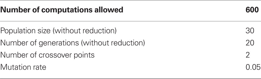
Table 2. Parameters that were the same for all genetic algorithm schemes.

TABLE 3

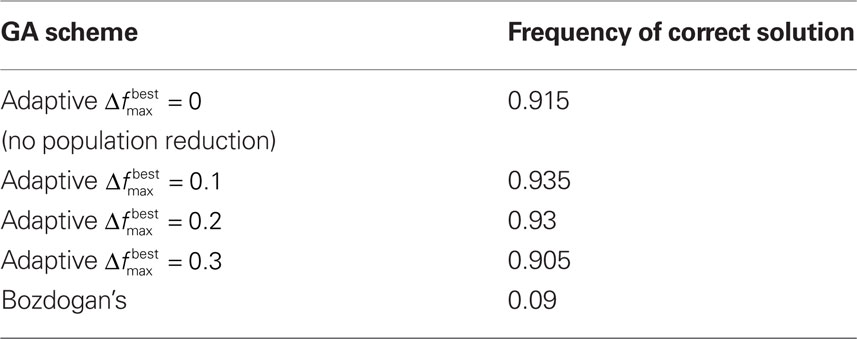
Table 3. The frequency of the correct model being selected over 200 trials. The first 4 schemes are with the modifications and the last is without.

Conclusion

While model selection remains to be a difficult procedure in case of a large number of parameters, using a GA to find the least complex model can be quite helpful. We have shown that our modifications to the original GA for model selection can yield strong results. Additionally, the GA approach (because of the use of ICOMP) is better at handling data in which collinearity exist than the traditional selection methods such as forward, backward, and stepwise selection. In particular it is clear that the modifications had a large effect on the accuracy of the GA. All of the GAs which implemented our modifications significantly outperformed Bozdogan’s GA. This seems to indicate that we may reduce computation and still get statistically the same accuracy if we employ diversification. In all trials, diversification never decreased accuracy. Along with the facts presented above and the fact that diversification is easy (and not costly) to implement, it is our recommendation that it be used for model selection using GAs.

Conflict of Interest Statement

The authors declare that the research was conducted in the absence of any commercial or financial relationships that could be construed as a potential conflict of interest.

References

Akaike, H. (1973). “Information theory and an extension of the maximum likelihood principle,” in Second International Symposium on Information Theory, eds B. N. Petrov and F. Csáki (Budapest: Académiai Kiadó), 267–281.

Boyce, D. E., Farhi, A., and Weischedel, R. (1974). Optimal Subset Selection: Multiple Regression, Interdependence, and Optimal Network Algorithms. New York: Springer-Verlag.

Bozdogan, H. (1988). “ICOMP: a new model-selection criterion,” in Classification and Related Methods of Data Analysis, ed. H. H. Bock (Amsterdam: Elsevier Science Publishers), 599–608.

Bozdogan, H. (2004). Statistical Data Mining and Knowledge Discovery. Boca Raton, FL: Chapman and Hall/CRC.

Fisher, R. A. (1930). The Genetical Theory of Natural Selection. Oxford: Clarendon Press.

Goldberg, D. E. (1989). Genetic Algorithms in Search, Optimization, and Machine Learning. Reading, MA: Addison-Wesley.

Hocking, R. R. (1976). The analysis and selection variables in linear regression. Biometrics 32, 1044.

CrossRef Full Text

Hocking, R. R. (1983). Developments in linear regression methodology: 1959–1982. Technometrics 25, 219–230.

CrossRef Full Text

Holland, J. H. (1975). Adaptation in Natural and Artificial Systems. Ann Arbor, MI: University of Michigan Press.

Mantel, N. (1970). Why stepdown procedures in variables selection. Technometrics 12, 591–612.

CrossRef Full Text

Moses, L. E. (1986). Think and Explain with Statistics. Reading, MA: Addison-Wesley.

Wilkinson, L. (1989). SYSTAT: The System for Statistics, Evanston, IL: SYSTAT.