Assessing periodicity of periodic leg movements during sleep

Background: Periodic leg movements (PLM) during sleep consist of involuntary periodic movements of the lower extremities. The debated functional relevance of PLM during sleep is based on correlation of clinical parameters with the PLM index (PLMI). However, periodicity in movements may not be reflected best by the PLMI. Here, an approach novel to the field of sleep research is used to reveal intrinsic periodicity in inter movement intervals (IMI) in patients with PLM. Methods: Three patient groups of 10 patients showing PLM with OSA (group 1), PLM without OSA or RLS (group 2) and PLM with RLS (group 3) are considered. Applying the “unfolding” procedure, a method developed in statistical physics, enhances or even reveals intrinsic periodicity of PLM. The degree of periodicity of PLM is assessed by fitting one-parameter distributions to the unfolded IMI distributions. Finally, it is investigated whether the shape of the IMI distributions allows to separate patients into different groups. Results: Despite applying the unfolding procedure, periodicity is neither homogeneous within nor considerably different between the three clinically defined groups. Data-driven clustering reveals more homogeneous and better separated clusters. However, they consist of patients with heterogeneous demographic data and comorbidities, including RLS and OSA. Conclusions: The unfolding procedure may be necessary to enhance or reveal periodicity. Thus this method is proposed as a pre-processing step before analyzing PLM statistically. Data-driven clustering yields much more reasonable results when applied to the unfolded IMI distributions than to the original data. Despite this effort no correlation between the degree of periodicity and demographic data or comorbidities is found. However, there are indications that the nature of the periodicity might be determined by long-range interactions between LM of patients with PLM and OSA.

Introduction

Periodic leg movements (PLM) during sleep are a sleep related phenomenon with periodic episodes of repetitive stereotypical movements of the lower extremities (American Sleep Disorder Association, 1993). PLM are more frequent in several sleep disorders, including restless legs syndrome (RLS, Montplaisir et al., 1997), narcolepsy (Moscovitch et al., 1993), rapid eye movement sleep behavior disorder (Fantini et al., 2002) as well as in disorders not primarily affecting sleep such as end stage renal disease (Benz et al., 2000). PLM during sleep are also documented in normal subjects (Pennestri et al., 2006) giving rise to the debate about functional relevance.

To determine the functional significance of PLM, the criteria used to score PLM during sleep are pivotal. Thus the criteria of detecting single leg movements (LM) as well as determining what constitutes periodicity may have a significant impact on the final result. According to the new standards PLM occur in a series of at least four LM and are separated by 5–90 s (Zucconi et al., 2006). An increased number of PLM during sleep with a PLM index (PLMI, i.e., the number of PLM per hour of total sleep time) of five or more is considered abnormal (American Academy of Sleep Medicine, 2005). Though the PLMI is taken to reflect periodicity in PLM in most studies, periodicity is not always obvious and PLMI may fail to report it. The definition of a period implicit in the PLMI encompasses inter movement intervals (IMI) from 5 to 90 s. This range of IMI may not be sufficiently restrictive to identify periodicity in LM and could allow randomly occurring LM to be considered periodic. On the other hand, IMI may change across the night (Coleman et al., 1980; Pollmächer and Schulz, 1993; Nicolas et al., 1998; Ferri et al., 2009) and PLM will be missed if period criteria are too narrow. Varying IMIs during night may lead to broad IMI distributions or to a distribution showing several local maxima. This makes a wide range of periods appear similarly prevalent, and thus hides intrinsic periodicity. Another way intrinsic periodicity may become difficult to detect is when pooling data from patients with different average periods of PLM. The definition of periodicity of LM is problematic and may not be sensitive enough. This lack of sensitivity could be one of the reasons for the ongoing debate about their functional relevance (Ancoli-Israel et al., 1991; Mendelson, 1996; Hornyak et al., 2004; Carrier et al., 2005; Högl, 2007; Mahowald, 2007).

A new statistical approach to analyze PLM was developed by Ferri et al. (2006b) who recommend to study the entire distributions of IMI rather than parametric measures as mean and standard deviation. They examined periodicity with a metric, termed the Periodicity Index (PI) measuring the percentage of LM appearing in series of periodic events. Instead of focusing on IMI frequency distributions the PI accounts for certain dependencies between subsequent IMIs. The PI was investigated for homogenous patient groups with RLS, narcolepsy/cataplexy and rapid eye movement sleep behavior disorder and without further potentially sleep relevant comorbidities or medication (Ferri et al., 2006a,b; Manconi et al., 2007). Based on different levels of the PI patients were divided into subgroups. For patients with narcolepsy/cataplexy and RLS a significantly different median of the PI was found (Ferri et al., 2006a). Very recently increased PI was also detected in a subgroup of patients with insomnia, for which no apparent cause could be found and enabled diagnosis of periodic leg movements disorder (PLMD, Ferri et al., 2009). Quantifiable aspects of PLM such as periodicity may serve to differentiate between clinical conditions and may eventually help capturing the nature of the underlying biological phenomenon (Rye, 2006). However, as afore mentioned, quantitative assessment of the periodicity of LM/PLM as measured by IMI is difficult because the empirical probability distribution may obscure underlying periodicity.

To date no study uses methods to enhance and reveal intrinsic periodicity before analyzing the statistics of IMI. We here employ the so-called unfolding procedure, which potentially uncovers intrinsic periodicity of LM data that is confounded by external influences. The unfolding procedure was originally developed in a branch of statistical physics called Random Matrix Theory (RMT) to study and compare the correlation between energy levels of heavy atomic nuclei and other complex quantum systems (see Brody et al., 1981; Guhr et al., 1998; Mehta, 2004, for comprehensive reviews). In the context of neurophysiology the concept was recently applied to the eigenvalue spectrum of the cross-correlation matrix calculated from multi-channel EEG (Seba, 2003; Müller et al., 2006; Baier et al., 2007).

In the present study we use the unfolding concept to assess the intrinsic periodicity of IMI of PLM examining a typical clinical patient cohort with PLM during sleep and different comorbidities from our database. Instead of studying the absolute IMI sizes, IMI are locally normalized to unit mean event spacing. Under these conditions the distribution of the spacings of randomly distributed events decays exponentially (Poisson distribution). In contrast, for strictly periodic systems the events are equally spaced. Fitting intermediate distributions, which interpolate between these extreme cases, to unfolded IMI distributions we quantify PLM periodicity.

Specifically, the goal of our study is to answer the following questions:

1. Does applying the unfolding procedure enhance and reveal periodicity that is not obvious from the measured IMI distribution?

2. Does periodicity differentiate between the clinical conditions of RLS, of OSA and of PLM without RLS or OSA?

3. Does data-driven clustering separate patients into different groups and are such groups clinically homogeneous?

Answering these questions could potentially provide further information about the clinical relevance of PLM during sleep.

Methods

Patients and Setting

Thirty patients were retrospectively evaluated at the Inselspital Bern Sleep Laboratory, all having a PLMI >15/h. Ten patients were diagnosed with PLM and OSA (group 1) with 10 or more obstructive apneas or hypopneas per hour of total sleep time. Ten patients were diagnosed with PLM without RLS or OSA (group 2). Five of these patients fulfilled the diagnostic criteria for PLMD (American Academy of Sleep Medicine, 2005). The last 10 patients had in addition RLS (group 3), fulfilling the minimal criteria accepted for the diagnosis of RLS (Allen et al., 2004). The presence of the following medical conditions was recorded: chronic cardiac or pulmonary disease, snoring, systemic hypertension, depression, obesity, Parkinsonism, headaches, fatigue, epilepsy, non-rapid eye movement parasomnia, idiopathic hypersomnia, and insomnia.

The case history analysis revealed that 17 of 30 patients were taking at least one medication on a regular basis at the time of evaluation. In group 1 (PLM with OSA) 2 patients out of 10 were not taking any medication, 2 patients were treated with opioids, 1 patient was taking betablocker and 1 patient paroxetin. The remaining 4 patients were taking medication not known to influence PLM. In group 2 (PLM without OSA or RLS) 6 patients out of 10 were not taking any medication, 1 patient was taking dopamine, 1 patient venlafaxine, trimipramin and betablocker and 1 patient mirtazapine and olanzapine. In group 3 (PLM with RLS) 5 patients out of 10 were not taking any medication, 1 patient was taking gabapentin and 1 patient was treated with mirtazapine and trazodone. The remaining 3 patients were taking medication not known to influence PLM. Tricyclic antidepressants, selective serotonin reuptake inhibitors and betablockers are considered to exacerbate PLM, whereas dopamine agonists, opioids, gabapentin, apomorphine are considered to reduce PLM (Allen et al., 2004).

Characteristics of patient groups are shown in Table 1 and Figure 1. The studied cohort shows a broad distribution of demographic data and sleep parameters. To assess statistical differences between the groups first a Kruskal–Wallis H-test for different central tendencies in the three groups (Siegel, 1956) was performed. If the differences were significant pairwise Mann–Whitney–Wilcoxon U-tests (Siegel, 1956) were subsequently performed in order to reveal where medians are different. Both tests were performed on significance level α = 0.01. For the Epworth Sleepiness Scale score (ESS) the H-test was not significant and for the PI it was only marginally significant (p = 0.049). With a few exceptions (see Figure 1) most pairwise U-tests were not significant. The reason is that the within group variability of the small groups (N = 10) was rather large and overshadowed the between group differences in most cases. However, these characteristics are representative for a typical patient cohort in a sleep clinic. Note that the highly significant differences with respect to AHI are due to the clinical a priori definition of the groups.

TABLE 1

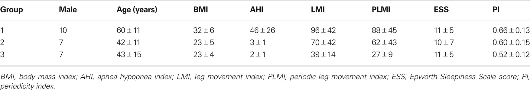
Table 1. Patient characteristics of group 1 (PLM with OSA), group 2 (PLM without OSA or RLS), and group 3 (PLM with RLS). Given are mean values and standard deviations. In Figure 1 the data is shown in box plot form.

FIGURE 1

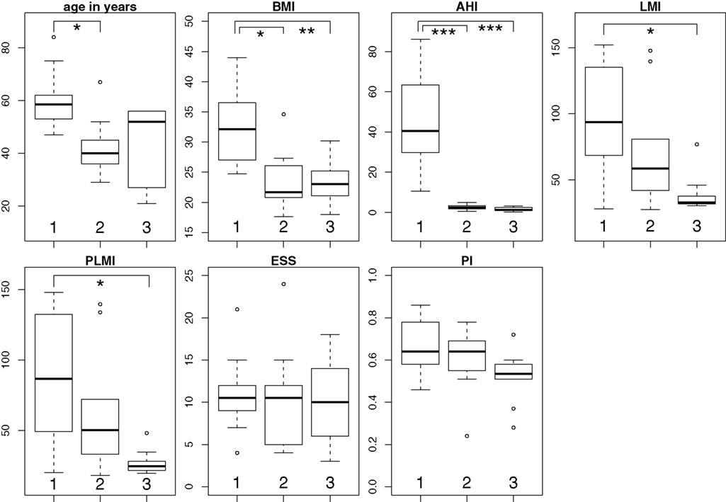
Figure 1. Box and whisker plots of the group-wise patient characteristics summarized in Table 1. The lower and upper lines of the boxes are the 25th and 75th percentiles (delimiting the “interquartile range”) of the sample and the line in the middle of the box represents the sample median. The “whiskers” are the lines extending above and below the box and show the extent of the rest of the sample. Outliers are shown as open circles. Significant differences of the medians (uncorrected pairwise Mann–Whitney–Wilcoxon U-tests) are indicated as follows: *p < 0.01, **p < 0.001, ***p < 0.0001. BMI, body mass index; AHI, apnea hypopnea index; LMI, leg movement index; PLMI, periodic leg movement index; ESS, Epworth Sleepiness Scale score; PI, periodicity index.

Polysomnography

Each patient underwent a diagnostic full night polysomnography (PSG). Patients had given their written informed consent for using their data for scientific purposes. Retrospective use of clinical data was approved by the local ethic committee.

Parameters recorded were electroencephalogram (EEG, minimal leads C4-M1, C3-M2, O2-M1, O1-M2, and additional F4-M1, F3-M2) respiration (nasal and oral airflow with thermistors, nasal pressure with a cannula, thoracic and abdominal respiratory movements with strain gauges, and oxygen saturation with finger oximetry), left and right electrooculogram, and three electromyogram (EMG) channels (submentalis muscle and right and left tibialis anterior muscles). EMG signals were sampled at 200 or 500 Hz, high pass filtered at 10 Hz and low-pass filtered at 45 or 100 Hz, respectively. Before the beginning of a recording a sleep technician checked that the amplitude of the EMG signal from the two tibialis anterior muscles was below 2 μV at rest and impedance was kept less than 5 kΩ. Sleep stages were scored by an experienced scorer (H. Gast) visually in 30 s epochs according to Rechtschaffen and Kales (1968).

Leg Movement Detection and Computation of Indices

Leg movements were first detected by the software Somnologica, Version 5.0.1. (Embla N7000 Recording Systems, Embla, Broomfield, CO, USA). The detections proposed by the automatic analysis were then edited by an experienced scorer (H. Gast) before computing the various parameters. All LM during sleep were included irrespective of association with arousals or apneas or hypopneas. LM while awake were not considered and thus a PLM sequence was terminated by intervening wakefulness. Otherwise the WASM standards for recording and scoring PLM during sleep were applied (Zucconi et al., 2006). A LM duration was at least 0.5 s and no longer than 10 s and IMI were calculated as the time elapsed from onset to onset of subsequent movements. LMs in the right and left leg were considered as simultaneous LMs and counted as only one LM if the separation between termination of the earlier and onset of the latter was equal or less than 0.5 s. LM were included in periodicity analysis if they occurred in a series of four or more events and if they were separated by IMI of more than 5 s and equal or less than 90 s.

The Unfolding Transformation

To characterize and quantify the intrinsic periodicity of PLM regardless of confounding systematic influences the “unfolding procedure,” which originates from RMT, was introduced to the field of PLM analysis for the first time. In the following a simple example is given, illustrating why unfolding may become necessary to reveal intrinsic periodicity. Thereafter the unfolding transformation is developed formally. Finally its usefulness is illustrated by applying it to model data.

Motivation

The ideal pendulum often serves as the paradigm of a periodic system. Event times T_i (i = 1,…,n) are defined as whenever the pendulum crosses the equilibrium from the left to the right. In the absence of any disturbing influences the events are equally spaced in time: T_i+1 = T_i + S. Here S = ΔT is the fundamental period of the pendulum which is related to the frequency f and the length l of the pendulum by According to this equation a shorter pendulum l′ < l has a higher frequency f′ and a smaller period ΔT′. If the pendulum is disturbed by environmental influences of any kind the spacings S_i = T_i+1 − T_i are no longer strictly equal but follow a distribution P₁(S), which we assume centered at ΔT. The characteristic of a (quasi-)periodic system is the narrowness of this distribution P₁(S). In contrast, broad distributions P₁(S) are identified with aperiodic systems where a characteristic frequency is absent.

To extend the example, suppose that the length of the pendulum becomes time dependent: l = l(T). If the length of the pendulum suffers a sudden change from l to l′ < l the distribution P₁(S) becomes bimodal with two centers at ΔT and ΔT′. If, however, a continuous but slow variation of l takes place over a large time period a broad distribution may result for P₁(S). Without doubt, the pendulum remains a periodic system. Solely, its intrinsic periodicity is obscured by an outer influence [its varying length l(T)] such that it can hardly be detected by measuring the spacing distribution P₁(S) in the most straight forward way.

Formal development

Instead one has to make use of a method designed for revealing and quantifying intrinsic fluctuations regardless of systematic trends of possibly unknown nature and origin. Originally it was introduced in the context of nuclear physics to put energy spectra of different atomic nuclei on the same footing before making comparison of certain fluctuation properties. Nowadays this method is extensively used in the field of quantum chaos. The crucial point consists in performing the so-called “unfolding procedure” (Brody et al., 1981; Haake, 1992; Guhr et al., 1998; Mehta, 2004) where the event times are transformed T_i → t_i such that the average distance (or time interval) between adjacent events becomes unity. Whereas a simple normalization can attain this goal on the global level, unfolding is designed to assure unit average spacing also locally. Different to the spacings S_i of the directly measured event times T_i the spacings s_i = t_i+1 − t_i of the unfolded t_i can be used to reveal intrinsic periodicities.

To develop the unfolding procedure formally, one starts from the density of n discrete events – in our case LM times:

Here δ(·) denotes the delta-distribution, i.e., a function that is very narrowly peaked at zero with unit integral. In the second identity we have split the event density into a smoothly T-dependent part that will subserve the unfolding distribution and a fluctuating residual. It is obvious that the probability P₁(S) of finding a neighboring event at a distance S from a selected one crucially depends on the event density ρ(T). Neighboring events will in general be closer if the event density is high than for low event density. To eliminate this influence, which may affect the inference of the system’s periodicity, one has to correct all spacings for the local smooth event density ρ_smooth(T).

Estimates of the event density ρ(T) from a finite amount n of data typically involve parameters like bin width and bin number. To avoid such influences it is more convenient to work with the parameter free cumulated event density:

that counts the number of events in the interval [ −∞,T], see Figure 2A for an illustration. At every event time T_i the so-called “staircase function” makes one step up. The unfolded events t_i are obtained from the smooth part of the cumulated event density by the transformation:

FIGURE 2

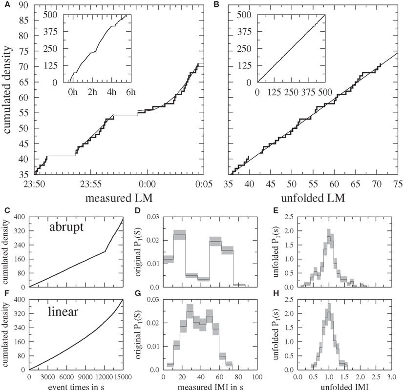
Figure 2. Top: Principle of the unfolding procedure. (A) In the inset the cumulated LM density (staircase function) is displayed for the whole night. Variations of the steepness of the curve due to varying event density ρ(T) are clearly visible. In the main part a detail of the staircase function is shown. LM runs of four or more spacings with IMI between 5 and 90 s are highlighted as fat curves. These pieces are fitted by low order polynomials (thin curves, here Δm = 4) which are subsequently used for the unfolding transformation Eq. 3. (B) Shows the unfolded cumulated LM density for the same data. Bottom: Demonstration of the unfolding for model data, see text. (C,F) The cumulated event densities are shown for abrupt and continuous linear change of the fundamental period ΔT. (D,G) are the measured IMI distributions for both cases. For the abrupt change of ΔT the intrinsic periodicity of the system is obscured by two pronounced peaks at S = 15 and 60 s whereas for the continuous linear decrease of ΔT a broad distribution results, where no significant peak can be identified. (E,H) show the unfolded IMI distributions of the same data. Here the intrinsic periodicity of the model becomes obvious in both cases from the single narrow peak.

By definition the mean spacing 〈s〉 of the t_i is locally equal to one along the whole unfolded event series.

The crucial issue of unfolding an event series is to find an appropriate estimate of N_smooth(T). In some physical cases an analytical formula for ρ_smooth(T) or N_smooth(T) is known and can be used in Eq. 3. Otherwise N_smooth(T) must be approximated from the experimentally measured data. To this end different strategies can be used, see e.g., discussion by Bruus and Anglés d’Auriac (1997). A common procedure consists of the so-called Gaussian broadening, where the delta-distributions in Eq. 1 are replaced by Gaussians. The constant or event-dependent widths are used as fit parameters. It has been found that Gaussian broadening tends to artificially introduce periodicity into event series at larger scales (Guhr et al., 1999; Gómez et al., 2002). To avoid this problem one can use a low order polynomial fit to the experimentally or numerically obtained cumulated event density N(T). The polynomial that minimizes square deviation from the staircase function of Eq. 2 is then used to perform the unfolding transformation Eq. 3, see e.g., Flores et al. (2000).

Here we proceed as follows, see Figure 2: according to the definition of PLM during sleep (Zucconi et al., 2006) we select LM runs of n ≥ 4 events occurring with IMI between 5 and 90 s from the whole series of LM times. An odd low order polynomial is fitted independently to each of these pieces. In order to prevent overfitting the staircase function with a polynomial of too high degree m, this parameter is given a logarithmic dependence on n:

Here the floor function ⌊·⌋ denotes the largest integer smaller than the argument. Eq. 4 guarantees that 1 ≤ m < n. It must be checked carefully that the dependence of the results on the particular choice of m is very weak. This can for example be done by lowering/rising m of Eq. 4 by Δm ∈ [−4, 4] (but respecting m ≥ 1), see Figures 3B–D. In addition to the m-dependence of the nearest neighbor spacing distribution P₁(s), which is extensively discussed in the present paper, also the next nearest neighbor distribution P₂(s) and the number variance Σ²(l) (Guhr et al., 1998; Mehta, 2004) should be considered. It measures long-range correlations between events by quantifying the variance of the number of events in pieces of (unfolded) length l and is known to be much more sensitive than the spacing distributions.

FIGURE 3

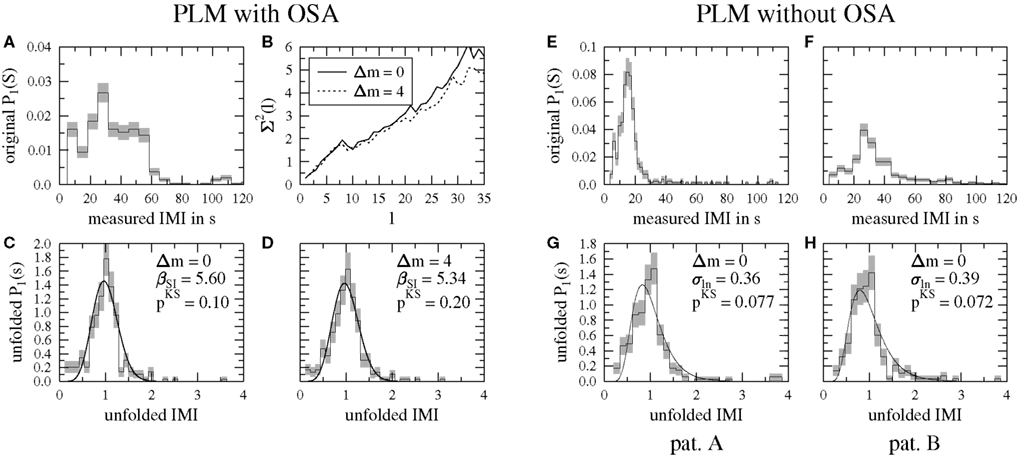
Figure 3. Examples for the usefulness of the unfolding. (A) Distribution of IMI before the unfolding procedure for the data of Figure 2A. IMI across the night with more than 6 h of sleep. Series of four or more leg movements with separation between 5 and 90 s have a very broad IMI distribution, suggesting a sequence with high randomness. (B) Insensitivity of the number variance to variations Δm of the degree of the fit polynomials. (C,D) After unfolding, IMI distribution became clearly peaked at 1 and the periodicity was thus correctly revealed. The unfolding procedure was insensitive to moderate variations of the polynomial degree m. As fully drawn lines, the best Scharf–Izrailev fit distributions (see Eq. 8 in Appendix) are shown. (E–H) Comparison of measured (E,F) and unfolded IMI distribution (G,H) for two patients with PLM without OSA or RLS. In patient A measured IMI show a narrow peak near 15 s whereas patient B has a much broader distribution with maximum near 30 s. Pooling data from both patients would have led to an even broader distribution. Applying the unfolding procedure the IMI distribution of both patients became very similar such that pooling patients conserved the characteristics of the distribution. As fully drawn lines the best fitting log-normal distributions (see Eq. 6 in Appendix) are shown.

Figure 2B shows the unfolded cumulated LM density after application of Eq. 3. Systematic trends are absent here. The data fluctuate around the function f(t) = t and the average event distance is 〈s〉 = 1 throughout the whole data set (reflecting local normalization).

Application to model data

The performance of the unfolding is illustrated at the example of the pendulum with variable length l and period ΔT discussed already above: n = 400 events were sampled from a pendulum subject to strong environmental noise, which was modeled by a Gaussian distribution of width 7.5 s. In the first case the center of the distribution is abruptly changed from 15 to 60 s after 200 events, whereas in the second case the change is continuously modeled by linear interpolation between the limiting values. The cumulated event densities are different, see Figures 2C,F. The linearly changing situation can be seen as a smooth version of the abrupt one with equal steepness at both ends of the curve. Comparison with Figure 2A shows that similar variations of the cumulated event density indeed occur in LM data.

In Figures 2D,G the measured IMI distributions P₁(S) are shown. Here and in subsequent histograms the optimal bin width (Scott, 1979) is used, which balances bias and variance by minimizing the mean squared error between measured data and histogram bins. It scales like n^−1/3 where n is the number of available data. The uncertainty of the number of events n(s) falling into a histogram bin centered at s is estimated by and symbolized as gray bars. Finally histograms (and errors) are downscaled in order to have unit sum In the abrupt situation (Figure 2D) two distinct, narrow peaks are visible. For the linearly changing case (Figure 2G) both have merged into a common, broader distribution. Different to the directly measured IMI distributions the unfolding procedure is able to reveal the intrinsic periodicity of the underlying system in both cases, see Figures 2E,H. Here clear peaks at s = 1 become visible after normalizing to the locally defined event density. Note that a simple global normalization would not succeed in either case.

Quantifying the Periodicity of the Unfolded IMI Distributions

Ferri et al. (2006b) have found that log-normal distributions fit the pooled measured IMI distributions best. Here it was investigated how the unfolded IMI distributions of individual patients can be fitted by standard distributions. To be independent of any kind of binning the least-squares fit was performed for the cumulated event densities. Like the unfolded IMI distributions P₁(s) all used fit distributions had mean 〈s〉 = 1. All of them depended on a single parameter, which controls the width of the distributions in monotonous manner. Consequently, these parameters could be used to quantify PLM periodicity. If an unfolded IMI distribution was more narrow than a second distribution we concluded that the PLM of were intrinsically more periodic.

For the log-normal distribution the fit parameter σ_ln determines the width of the distribution directly, see Appendix for details and formulae. The log-normal distribution neither contains the exponentially decaying Poissonian case as a limit nor is it used in RMT for description of spacing distributions. Here it was used in order to tie in with previous work by Ferri et al. (2006b). Excluding one possible parametrization of the IMI distribution in favor of another might help to learn about the nature of the interaction (e.g., long-range vs. short-range) between subsequent LM in PLM series. Therefore we probed in addition two RMT spacing distributions that can be derived rigorously for classical one-dimensional particle gases on rings (Dyson gases), see Appendix for details and formulae. The Scharf–Izrailev distribution (Izrailev, 1988; Scharf and Izrailev, 1990) describes the spacings for Dyson gases with long-range interactions between all particles at temperature 1/β_SI. Similarly, starting from Dyson gases with short-range interactions between neighboring particles at temperature 1/β_sP one arrives at the semi-Poisson distribution (Bogomolny et al., 1999). For both distributions a decreasing temperature (increasing fit parameters β_SI and β_sP in the present context) translates into decreasing width. Both distributions interpolate between the exponentially decaying Poissonian (β_SI = β_sP = 0) and peaked distributions (β_SI, β_sP > 0).

To investigate which distribution fits the empirical distributions of unfolded IMI best, the non-parametric Kolmogorov–Smirnov (KS) test (Press et al., 1992) was employed. It gives a distance d^KS ≥ 0 between the cumulated density of the sample distribution and the one of the functions given in explicit form in the Appendix (Eq. 7 for log-normal, the numerical integral of Eq. 8 for Scharf–Izrailev or Eq. 11 for semi-Poisson) and a significance 0 ≤ p^KS ≤ 1. The latter depends on d^KS as well as on the size n of the distribution and gives the probability that a distance d^KS or larger is found although the null hypothesis of equal distributions is correct. We considered a fit as a good one if p^KS ≥ 0.1 and discarded it otherwise.

In order to rank the performance of the fit distributions for clinical patient groups and automatically defined clusters (see Automated Similarity Clustering) we followed two approaches. The first one used the average p-value 〈p^KS〉 of a fit distribution over the individuals of the selected group. For the second one we gave credits to the fit distributions in the following way: zero credits if for a patient’s unfolded IMI distribution p^KS < 0.1, one credit if p^KS ≥ 0.1, three credits for the best fit and two credits for the second best fit. In order to make the total number of credits comparable across groups or clusters it was divided by the number of group or cluster members.

Automated Similarity Clustering

Besides interpreting the distributions of measured and unfolded IMI for patients and clinically defined patient groups it was in addition investigated if it is possible to partition the total of the 30 data sets in a way that maximizes similarity within and differences between the groups. To quantify the similarity of two IMI distributions P_μ and P_ν the KS test was employed again, now in its version for two samples (Siegel, 1956; Press et al., 1992). As before, it results in a distance and a significance Here depends on as well as on the sizes n_μ and n_ν of the distributions. In the present paper was used to quantify the similarity of two distributions with a single number in [0, 1] (0 for non-overlapping distributions and 1 for identical ones) in a size independent manner.

For automated similarity clustering on basis of the matrix with entries the contrast turned out too weak. To deal with this problem the transformation:

was performed, where and σ_p denote the average and standard deviation of the off-diagonal respectively. This monotonic transformation sharpened the contrast by enlarging elements larger than average and decreasing elements smaller than average.

On the basis of these x_μν the recently developed cluster participation vector (CPV) algorithm (Rummel et al., 2007, 2008; Rummel, 2008) was employed. It operates on the eigenvectors of the symmetric similarity matrix with elements 0 ≤ x_μν ≤ 1 (with ones on the diagonal) and performs two tasks in a fully data-driven manner. First, the number K of clusters present in the data can be estimated from features of all eigenvectors rather than pre-specifying it on the basis of previous knowledge. For this step another Kolmogorov–Smirnov test must be carried out, for which a significance level of α = 0.01 was chosen. Second, the data sets are attributed to the clusters on basis of the components of suitable linear combinations of the eigenvectors belonging to the K largest eigenvalues of the similarity matrix. The CPV algorithm has been tested extensively and was shown to outperform traditional approaches especially in situations with clusters that show sizable inter-cluster similarities.

Results

Unfolding in Single Patient Data

Applying the unfolding procedure Eq. 3 revealed periodicity and allowed pooling of data. Figure 3A shows the example of a measured IMI distribution of a 75-year-old male with PLM and OSA (BMI = 27.3, AHI = 63.4, LMI = 77.1, PLMI = 70.7, PI = 0.62). The distribution of measured IMI is broad and almost flat between 5 and 60 s with only a small peak near IMI = 30 s. This distribution suggests a non-periodic system with all periods between 5 and 60 s appearing similarly often. Note that a small sample of IMI drawn with a random number generator (the prototype of a non-periodic system) from a uniform distribution between 5 and 60 s (and zero outside) could lead to a similar distribution. By definition such a LM series has PI = 1 although it is purely random (Ferri et al., 2006b).

Unfolding the data showed a clear contrast with a distinct peak at 1, revealing periodicity of LM that was previously hidden (Figures 3C,D). The intrinsically periodic character of the data was obscured in Figure 3A by the different slopes of the staircase function (see this patients’ event times in Figure 2A), which represent different kinds of external influences on IMI duration such as, e.g., sleep stage or time elapsed after falling asleep. Both, the number variance (Figure 3B) and the unfolded IMI distribution were rather insensitive to the particular choice of the polynomial degree of Eq. 4. Increasing m for every piece by Δm = 4 led to very similar results. For both versions of the unfolded IMI distribution the p-value of a Scharf–Izrailev fit [see Eq. 8 in Appendix] was largest as compared to the remaining fit distributions and exceeds 0.1. Therefore the Scharf–Izrailev fit was accepted for further analysis, see below.

Pooled IMI from different patients may become broad and therefore suggest high randomness, i.e., non-periodic distribution of IMI. The measured IMI distribution of two patients showing PLM without OSA or RLS are given in Figures 3E,F. Patient A (67 years, male, BMI = 27.3, AHI = 1.0, LMI = 147.8, PLMI = 139.6, PI = 0.56) had a pronounced peak at 15 s whereas the distribution of patient B (45 years, male, BMI = 26.1, AHI = 2.4, LMI = 60.3, PLMI = 54.2, PI = 0.74) was much broader and peaked near 30 s. Pooling the measured data of these two patients would have led to an even broader distribution. After unfolding (Figures 3G,H) the IMI distribution of both patients became similar and the estimated values of the log-normal fit parameters σ_ln were very close. Pooling them would not alter the character of the distribution. The log-normal distribution (see Eq. 6 in Appendix) turned out as the best fit distribution in both cases and is indicated as fully drawn lines in Figures 3G,H. Although the log-normal distribution fitted the data better than the alternatives, both p-values remained below 0.1. Therefore these examples were excluded from our further analysis of the fit parameter σ_ln.

Unfolding in Patient Groups 1 to 3

The pooled measured IMI of patient group 1 (PLM with OSA) showed the most peaked distribution whereas patient group 3 (PLM with RLS) showed the broadest distribution, see Figure 4. The shape of all three distributions was clearly different. In contrast, the unfolded IMI distributions in groups 2 (PLM without OAS or RLS) and 3 showed much more similar shape.

FIGURE 4

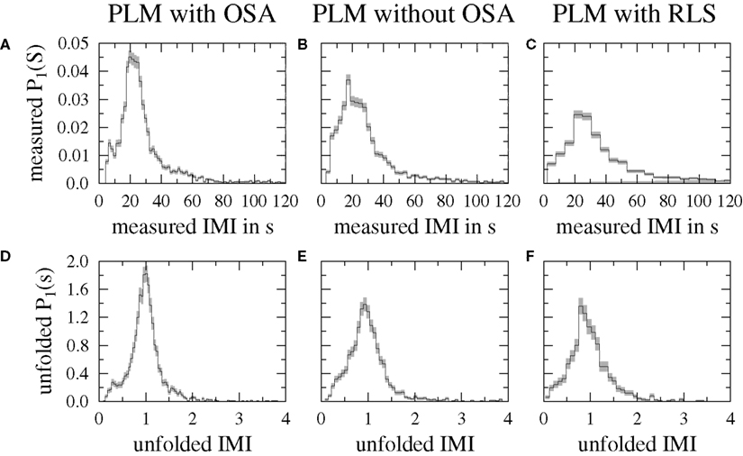
Figure 4. Pooled measured (A–C) and unfolded IMI distribution (D–F) for three clinically defined patient groups.

The majority of the unfolded IMI distributions of individual patients belonging to the three patient groups could be fitted well by the functions given in the Section “Methods.” Patient group 3 (PLM with RLS) could be fitted best by the log-normal distribution according to both ranking criteria (Table 2). This result confirmed a finding by Ferri et al. (2006b) who successfully fitted the pooled measured IMI distributions of RLS patients by log-normal distributions. For patient group 1 (PLM with OSA) the Scharf–Izrailev distribution turned out as a much better fit than the semi-Poisson or the log-normal distribution, implying that long-range interactions between LM could play a role in this patient group. For patient group 2 (PLM without OSA or RLS) there was disagreement between the maximum number of credits and the maximal average p-value 〈p^KS〉 thus implying fundamental differences in the shape of the unfolded IMI distributions within these patient groups. These differences were accounted for best by describing the data of different patients with different fit distributions. Overall, unfolded IMI distributions were fitted best by the Scharf–Izrailev distribution closely followed by the semi-Poisson distribution, see Table 2. With the exception of the RLS group the log-normal distribution led to the worst fits.

TABLE 2

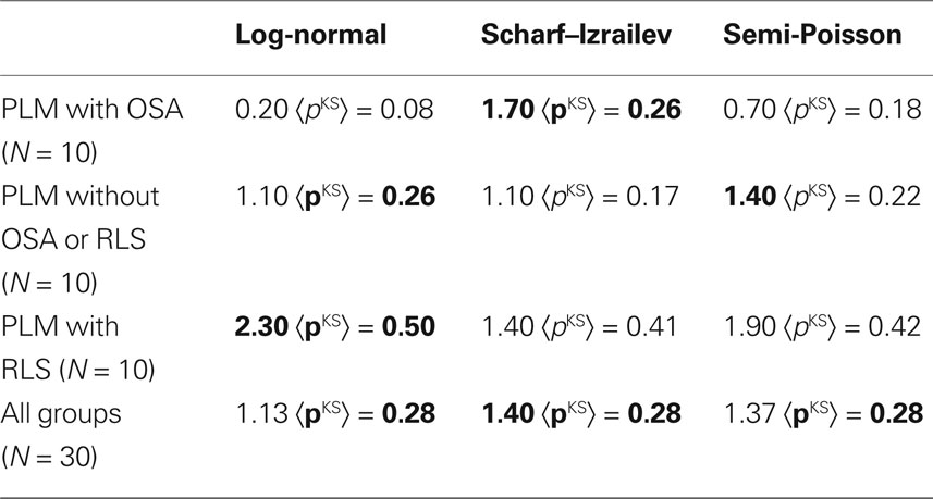
Table 2. Ranking of the goodness-of-fit for the clinical groups. The left numbers are the group-wise average number of credits whereas the right number is the average significance of the KS test. The group-wise best fit is displayed in boldface.

A Kruskal–Wallis H-test was carried out for group-wise different central tendency of the accepted (p^KS ≥ 0.1) fit parameters σ_ln, β_SI, and β_sP without finding significant differences (p > 0.1). Finally, it was found that the fit parameter σ_ln of the N = 17 good fits of the log-normal distribution anti-correlated significantly (non-parametric Spearman correlation, p < 0.01) with the patients’ BMI, suggesting more overweight patients show a more narrow distribution, see Table 3. Investigation on a larger patient cohort is necessary to decide whether age, subjective sleepiness and PI (which turn out marginally significant, p < 0.05) are also candidates for significant anti-correlation. Very similar tendencies toward non-parametric correlation are present for the N = 19 accepted fit parameters β_SI of the Scharf–Izrailev fit (now correlation instead of anti-correlation). In contrast no significant correlation with demographic data was found for the N = 18 accepted semi-Poisson fits.

TABLE 3

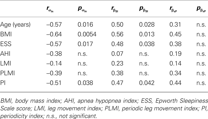
Table 3. Spearman’s rank-order correlation between the fit parameters of the log-normal, the Scharf–Izrailev and the semi-Poisson distribution and demographical data.

Data-Driven Clustering

Visually comparing the measured and unfolded IMI distributions within clinically defined patient groups showed large dissimilarities occasionally, see Figure 3E and F for an example of measured data. On the other hand very similar IMI distributions were found for patients from different clinically defined groups. Therefore the following questions arose:

1. Is it possible to define new groups according to the shape of the IMI distributions using cluster algorithms?

2. Is there a common/are there shared clinical or demographic features that may cause the cluster formation?

To address question 1 the CPV clustering algorithm on basis of the similarities between the measured IMI distributions was employed (see Methods). Figure 5A shows the similarity matrix of the original pairwise Kolmogorov–Smirnov significances Data was ordered according to the clinically defined groups: PLM with OSA (a to j), PLM without OSA or RLS (k to t), PLM with RLS (u to δ). Apart from the diagonal and some exceptions in the group PLM with RLS, similarities were small. Application of Eq. 5 sharpens the contrast (Figure 5B). However, using these x_μν for CPV clustering did not reveal a distinct cluster pattern. Determining the number of clusters in data-driven manner led to K = 10 clusters, the strongest one comprising the data sets o, w, y, and δ (data not shown). The second strongest cluster comprised data sets t, u, and x. Three clusters contained only two data sets, like, e.g., m and α. Figure 5B shows large elements of the similarity matrix x_μν connecting these data sets. However, most importantly, none of the clusters was homogeneous consisting of patients belonging to the same patient group or sharing any other clinical or demographical characteristic. In summary, clustering on the basis of the similarities of measured IMI distributions did not seem to lead to clinically conclusive results.

FIGURE 5

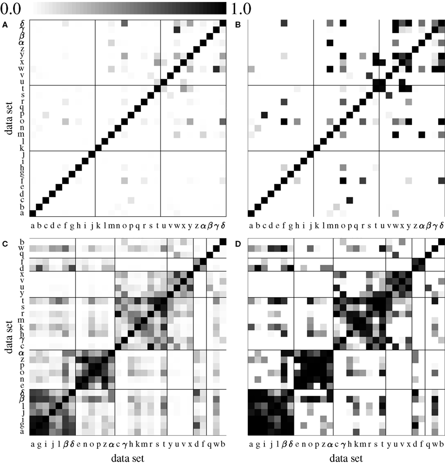
Figure 5. Matrix of similarities of the distributions. Top: Similarities (A) and x_μν (B) of measured IMI distributions. Data sets were ordered according to patient groups and group boundaries are indicated by fully drawn lines: PLM with OSA (a to j), PLM without OSA or RLS (k to t), PLM with RLS (u to δ). The similarity in the group PLM with RLS was higher than for the remaining groups. Data-driven clustering predominantly depicted small clusters (see Methods). Bottom: Similarities (C) and x_μν (D) of the unfolded IMI distributions were much larger. Data-driven clustering found several large clusters. For illustration purposes, the channels were ordered according to five automatically detected clusters comprising data sets a to δ (cluster A, seven members), e to α (cluster B, six members), c to t (cluster C, eight members), y to x (cluster D, four members) as well as d and f (cluster E, two members). Cluster boundaries are again indicated by fully drawn lines.

Cluster participation vector clustering was repeated on the basis of the similarity of the unfolded IMI distributions. The elements and x_μν of the similarity matrices shown in Figures 5C,D were in general much larger than for the measured data. For better visual representation the data sets were rearranged according to K = 5 clusters that were found by the CPV algorithm. The clusters comprised data sets a to δ (cluster A, seven members), e to α (cluster B, six members), c to t (cluster C, eight members), y to x (cluster D, four members) and d and f (cluster E, two members). Data sets q, w, and b remained unclustered. Data set β (female, 21 years, RLS) had only slightly stronger similarities with cluster A than with B and therefore connected both clusters. Similarly, clusters A and E as well as C and D were strongly interconnected.

Figure 6 shows the pooled unfolded IMI distributions for the clusters A to E of Figures 5C,D. Clusters B and E had the narrowest distribution notwithstanding a weak connection. Cluster E was more strongly connected with cluster A via data set d (male, 49 years, OSA), see Figure 5D. The strongly connected clusters C and D had similar distributions.

FIGURE 6

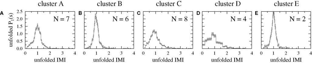
Figure 6. Pooled unfolded IMI distributions of the five automatically detected similarity clusters. The membership of the data sets in the clusters becomes transparent from the similarity matrices shown in Figures 5C,D.

Analyzing medical conditions or medication that exacerbate or reduce PLM within these clusters did not reveal any common cluster specific features. Only the Kruskal–Wallis H-test for cluster-wise different central tendency of the PI (Ferri et al., 2006b) was significant on significance level α = 0.01. For the cluster medians of the PI significant pairwise differences between clusters A and D as well as between clusters B and D (U-test) were found. Note that these cluster pairs were especially weakly interconnected in Figure 5D. In addition PI medians were marginally different for the following combinations: C vs. D (p = 0.016) and C vs. E (p = 0.044). The medians of the demographic data were only marginally significantly different. BMI and PLMI: cluster A vs. D (p = 0.042); AHI: cluster B vs. D (p = 0.038). It is interesting to note that Ferri’s PI was the only quantity that showed significant differences between the automatically found similarity clusters. Mind that for the clinically defined groups no significant difference of PI was found (Figure 1).

Subsequently the analysis of the goodness-of-fit of the one-parameter fit distributions given in the Section “Methods” for the automatically defined similarity clusters was repeated, see Table 4. With the exception of cluster C there was agreement between both ranking methods for all clusters. In addition now the cluster-wise average p-value of the best fit distribution was larger, implying that clustering automatically groups patients whose IMI can be fitted best by the same distribution.

TABLE 4

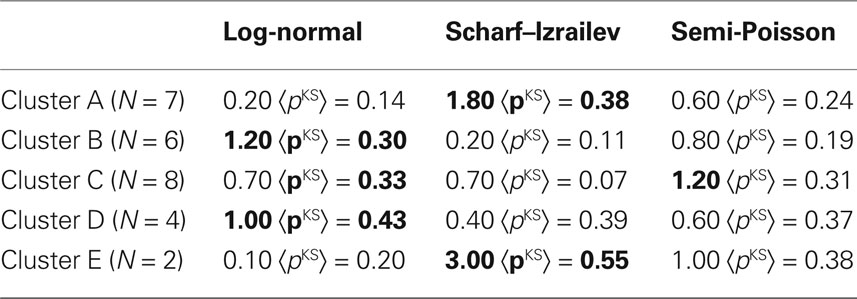
Table 4. Ranking of the goodness-of-fit for the automatically defined clusters. Displayed are the same quantities as in Table 2. The cluster-wise best fit is displayed in boldface.

For clusters B and D the log-normal distribution delivers clearly the best fit. However, this does not imply the fit parameter σ_ln was the same in both clusters (see Figure 6): σ_ln = 0.25 ± 0.03 for cluster B and σ_ln = 0.55 ± 0.06 for cluster D (marginally significant difference of medians, U-test: p = 0.029). Note that for the clinically defined patient groups differences in σ_ln were not significant (p > 0.1). Note also that the apparently similar unfolded IMI distributions of clusters B and E were best fitted by different fit distributions. This illustrates how automatic clustering reveals features of the data that cannot be obtained by visual inspection. For the unfolded IMI distributions of patients belonging to clusters A and E the Scharf–Izrailev distribution had the best fit performance. Here the fit parameters had different tendencies in both clusters (A: β_SI = 5.21 ± 1.26, E: β_SI = 9.76 ± 0.34), however, due to the small cluster sizes the difference did not reach significance (U-test: p = 0.095).

Discussion

In the present study, we applied for the first time the unfolding procedure of RMT to analyze PLM data. Our first objective was to test whether unfolding would enhance and reveal intrinsic periodicity that is not obvious from the measured IMI distribution. Indeed, we found that applying this procedure in single patients improved detection of periodicity, which was hidden within a broad distribution of measured IMI (Figures 3A,C,D). Thus, this result underlines the usefulness of unfolding for the detection of periodicity in neurophysiological time series. The broad range of measured IMI may be due to their dependence on the time of night and sleep stage (Coleman et al., 1980; Culpepper et al., 1992; Pollmächer and Schulz, 1993). In addition, the IMI probably may also depend on the time of intake of medication and its pharmacokinetics influencing motor activity in sleep.

Because unfolding may be necessary to enhance and reveal periodicity, we propose this method as an important pre-processing step before analyzing PLM. Note that this recommendation holds independently from the method used for recording the LM, be it EMG (as in our study) or other methods like the recently applied Emfit sensor (Rauhala et al., 2009). Pooling of measured IMI may also broaden a group’s IMI distribution, whereas applying the unfolding procedure before pooling the patients’ data retains their characteristics (Figures 3G,H). Technically, it is important to note that our choice of the degree m of the fit polynomial according to Eq. 4 prevents overfitting the data. Allowing for variations Δm ∈ [−4, 4] we have shown in addition that the results are robust against variation of the particular choice of m (Figures 3B–D).

Here we investigated PLM periodicity by focusing on the shape of IMI distributions through the unfolding procedure. In patients with PLM and RLS Ferri et al. (2006b) found a bimodal distribution of measured IMI with the lower peak considerably below 10 s. This differs from our finding of a single-peaked distribution of measured IMI in patient group 3 (Figure 4C). The reason for this difference might be that in contrast to our analysis these authors based their calculation of LM distribution on all IMI intervals >0.5 s in contrast to the WASM definition of PLM during sleep applied to our data (Zucconi et al., 2006).

PLM associated with OSA and RLS show distinct IMI characteristics (Culpepper et al., 1992; Briellmann et al., 1997). Therefore our second objective was to test whether periodicity could differentiate between the clinical groups containing patients with PLM and OSA (group 1), PLM and RLS (group 3) and PLM without RLS or OSA (group 2). PLM periodicity was assessed by fitting one-parameter distributions to the unfolded IMI distributions of individual patients. The pooled IMI distributions of the three groups appeared very similar (Figures 4D–F) and none of the patients’ fit parameters σ_ln, β_SI, and β_sP was significantly different between the groups. These results suggest that the degree of periodicity as quantified by these parameters is not related to the comorbidity (OSA or RLS). However, patients within groups were heterogeneous in terms of medication and comorbidities, thus representing a typical patient cohort in a sleep clinic. This heterogeneity contrasts with other studies that investigated patients with RLS and/or PLM excluding patients with medication influencing motor activity during sleep or significant sleep disorder or major comorbidities (Allen et al., 2004; Garcia-Borreguero et al., 2004; Hornyak et al., 2004; Ferri et al., 2006a,b, 2009; Manconi et al., 2007).

Non-parametric correlation between the fit parameters and demographic patient data showed a significantly more narrow IMI distribution, i.e., a more pronounced periodicity, for overweight patients. BMI of patient group 1 (PLM with OSA) was significantly higher compared to groups 2 (PLM with RLS) and 3 (PLM without RLS or OSA), see Figure 1.

In contrast to the degree of periodicity (as defined by the values of the fit parameters σ_ln, β_SI, and β_sP), its nature (as defined by the best fit distribution) was different between patient groups. We confirmed the result by Ferri et al. (2006b) that IMI distributions of patients suffering from RLS (here unfolded patient-wise distributions instead of pooled measured ones) can be fitted best by the log-normal distribution. On the contrary, the IMI distributions of patients in the OSA group could best be described by the Scharf–Izrailev distribution. Keeping in mind that this distribution can be derived for Dyson gases with long-range interaction between the particles (Izrailev, 1988; Scharf and Izrailev, 1990) this might imply a certain role of long-range interactions across several LM in these patients.

Our third objective was to test whether a data-driven cluster analysis would separate patients into different groups. Measured and unfolded IMI distributions showed considerable dissimilarity within groups, while patients from different groups occasionally showed similar distributions. Therefore a possible definition of data-driven group formation could be derived from the shape of the IMI distributions. Data-driven clustering of unfolded IMI distributions of PLM had not been described before and yielded five similarity clusters. We found that the PI (Ferri et al., 2006b) is the only quantity that shows significant differences between these clusters. This may be due to both approaches aiming at quantifying PLM periodicity.

However, the clusters were heterogeneous with respect to clinical and most demographic data. It remains unclear, which pathophysiological mechanism is responsible for the different shapes of the IMI distributions. One might speculate that the presumed neuronal central pattern generator responsible for the occurrence of PLM (Parrino et al., 1996, 2006; Guggisberg et al., 2007), is differentially influenced by medication and comorbidities such as RLS or OSA.

Analysis of the goodness-of-fit of the one-parameter fit distributions for the automatically defined similarity clusters showed the log-normal distribution to yield the best fit for two of the clusters (10 patients altogether). Also the Scharf–Izrailev distribution fitted two of the clusters best (9 patients altogether). Furthermore the apparently similar unfolded IMI distributions of two clusters (Figures 6B,E) were best fitted by different distributions. This finding indicates that subtle differences of periodicity may not be detected visually.

It remains to be investigated, whether and how applying the unfolding procedure to larger and more homogeneous patient groups allows the association between PLM and clinical significance. Furthermore, an interesting question is whether application of more sophisticated RMT tools like, e.g., the number variance or the related but more stable Dyson–Mehta statistic Δ₃(l) (not used in the present publication) helps to clarify the open questions of the clinical relevance of PLM and the nature of interaction between subsequent LM in PLM series. Both, and Δ₃(l) can be used to measure long-range correlations between IMI and consequently could complement the Markovian analysis carried out by Ferri et al. (2006a,b) from a methodological point of view.

Appendix

One-Parameter Fit Distributions

Here we give the distributions used for fitting unfolded IMI distributions in explicit form. The Scharf–Izrailev and semi-Poisson distributions can be derived rigorously from the model assumptions of one-dimensional particle gases on a ring (Dyson gas) with long-range and short-range interactions, respectively. As a consequence, excluding one distribution in favor of the other one, could help to understand mechanisms underlying LM series.

Log-normal distribution

Similar to Ferri et al. (2006b) the log-normal distribution is used (see e.g., Limpert et al., 2001) with mean 〈s〉 = 1 and a fit parameter σ_ln that controls the width:

Its cumulated density is given by

Scharf–izrailev distribution

A heuristic formula for interpolating between the exponentially decaying Poisson and the peaked Wigner distribution results from the spacing statistics of Dyson gases with long-range interactions at temperature 1/β_SI (Izrailev, 1988; Scharf and Izrailev, 1990):

Here increasing parameter β_SI (decreasing “temperature”) implies decreasing width of the distribution. The constants A_SI and B_SI must be calculated numerically for given β_SI by demanding normalization and mean unit spacing Also the cumulated density is integrated numerically. For integer values of β_SI the Scharf–Izrailev distribution coincides with well known distributions of RMT. For β_SI = 0 the Poisson distribution and for β_SI = 1 the Wigner distribution are reproduced.

Semi-poisson distribution

The semi-Poisson distribution describes the spacing statistics of Dyson gases with short-range interaction at temperature 1/β_sP (Bogomolny et al., 1999) as well as incomplete spectra of complex systems (Hernández-Saldaña et al., 1999). In addition it has been found empirically that distributions of (unfolded) car distances on highways can be fitted by the semi-Poisson distribution (Krbalek et al., 2001):

Also here increasing parameter β_sP (decreasing “temperature”) decreases the distribution’s width. The normalization is given by

Its cumulated density is given by the incomplete Gamma function P(·,·):

For β_sP = 0 again the Poisson distribution is reproduced.

Conflict of Interest Statement

The authors declare that the research was conducted in the absence of any commercial or financial relationships that could be construed as a potential conflict of interest.

Acknowledgments

This work was supported by Deutsche Forschungsgemeinschaft, Germany (grant RU 1401/2-1) and Schweizerischer Nationalfonds, Switzerland (project 320030_122010). Markus Müller receives support by CONACyT, Mexico (project 48500).

References

Allen, R., Becker, P. M., Bogan, R., Schmidt, M., Kushida, C. A., Fry, J. M., Poceta, J. S., and Winslow, D. (2004). Ropinirole decreases periodic leg movements and improves sleep parameters in patients with restless legs syndrome. Sleep 27, 907–914.

Pubmed Abstract | Pubmed Full Text

American Academy of Sleep Medicine. (2005). International Classification of Sleep Disorders: Diagnostic and Coding Manual, 2nd Edn. Westchester: American Academy of Sleep Medicine.

American Sleep Disorder Association. (1993). Atlas task force. Recording and scoring of leg movements. Sleep 16, 748–759.

Pubmed Abstract | Pubmed Full Text

Ancoli-Israel, S., Kripke, D. F., Klauber, M. R., Mason, W. J., Fell, R., and Kaplan, O. J. (1991). Periodic limb movements in sleep in community-dwelling elderly. Sleep 14, 496–500.

Pubmed Abstract | Pubmed Full Text

Baier, G., Müller, M., Stephani, U., and Muhle, H. (2007). Characterizing correlation changes of complex pattern transitions: the case of epileptic activity. Phys. Lett. A 363, 290–296.

CrossRef Full Text

Benz, R. L., Pressman, M. R., Hovick, E. T., and Peterson, D. D. (2000). Potential novel predictors of mortality in end-stage renal disease patients with sleep disorders. Am. J. Kidney Dis. 35, 1052–1060.

Pubmed Abstract | Pubmed Full Text | CrossRef Full Text

Bogomolny, E. B., Gerland, U., and Schmit, C. (1999). Models of intermediate spectral statistics. Phys. Rev. E 59, R1315–R1318.

CrossRef Full Text

Briellmann, R. S., Mathis, J., Bassetti, C., Gugger, M., and Hess, C. W. (1997). Patterns of muscle activity in legs in sleep apnea patients before and during nCPAP therapy. Eur. Neurol. 28, 113–118.

CrossRef Full Text

Brody, T., Flores, J., French, J., Mello, P., Pandey, A., and Wong, S. (1981). Random-matrix physics: spectrum and strength fluctuations. Rev. Mod. Phys. 53, 385–479.

CrossRef Full Text

Bruus, H., and Anglés d’Auriac, J.-C. (1997). Energy level statistics of the two-dimensional hubbard model at low filling. Phys. Rev. B 55, 9142–9159.

CrossRef Full Text

Carrier, J., Frenette, S., Montplaisir, J., Paquet, J., Drapeau, C., and Morettini, J. (2005). Effects of periodic leg movements during sleep in middle-aged subjects without sleep complaints. Mov. Disord. 20, 1127–1132.

Pubmed Abstract | Pubmed Full Text | CrossRef Full Text

Coleman, R. M., Pollak, C. P., and Weitzman, E. D. (1980). Periodic movements in sleep (nocturnal myoclonus): relation to sleep disorders. Ann. Neurol. 8, 416–421.

Pubmed Abstract | Pubmed Full Text | CrossRef Full Text

Culpepper, W. J., Badia, P., and Shaffer, J. I. (1992). Time-of-night patterns in PLMS activity. Sleep 15, 306–311.

Pubmed Abstract | Pubmed Full Text

Fantini, M., Michaud, M., Gosselin, N., Lavigne, G., and Montplaisir, J. (2002). Periodic leg movements in REM sleep behavior disorder and related autonomic and EEG activation. Neurology 59, 1889–1894.

Pubmed Abstract | Pubmed Full Text

Ferri, R., Gschliesser, V., Frauscher, B., Poewe, W., and Högl, B. (2009). Periodic leg movements during sleep and periodic limb movement disorder in patients presenting with unexplained insomnia. Clin. Neurophysiol. 120, 257–263.

Pubmed Abstract | Pubmed Full Text | CrossRef Full Text

Ferri, R., Zucconi, M., Manconi, M., Bruni, O., Ferini-Strambi, L., Vandi, S., Montagna, P., Mignot, E., and Plazzi, G. (2006a). Different periodicity and time structure of leg movements during sleep in narcolepsy/cataplexy and restless legs syndrome. Sleep 29, 1587–1594.

Ferri, R., Zucconi, M., Manconi, M., Plazzi, G., Bruni, O., and Ferini-Strambi, L. (2006b). New approaches to the study of periodic leg movements during sleep in restless legs syndrome. Sleep 29, 759–769.

Flores, J., Horoi, M., Müller, M., and Seligman, T. H. (2000). Spectral statistics of the two-body random ensemble revisited. Phys. Rev. E 63, 026204.

CrossRef Full Text

Garcia-Borreguero, D., Larrosa, O., de la Llave, Y., Granizo, J. J., and Allen, R. (2004). Correlation between rating scales and sleep laboratory measurements in restless legs syndrome. Sleep Med. 5, 561–565.

Pubmed Abstract | Pubmed Full Text | CrossRef Full Text

Gómez, J. M. G., Molina, R. A., Relano, A., and Retamosa, J. (2002). Misleading signatures of quantum chaos. Phys. Rev. E 66, 036209.

CrossRef Full Text

Guggisberg, A. G., Hess, C. W., and Mathis, J. (2007). The significance of the sympathetic nervous system in the pathophysiology of periodic leg movements in sleep. Sleep 30, 755–766.

Pubmed Abstract | Pubmed Full Text

Guhr, T., Ma, J.-Z., Meyer, S., and Wilke, T. (1999). Statistical analysis and the equivalent of a Thouless energy in lattice QCD Dirac spectra. Phys. Rev. D 59, 054501.

CrossRef Full Text

Guhr, T., Müller-Groeling, A., and Weidenmüller, H. A. (1998). Random-matrix theories in quantum physics: common concepts. Phys. Rep. 299, 189–425.

CrossRef Full Text

Haake, F. (1992). Quantum Signatures of Chaos, 2nd Edn. Berlin: Springer.

Hernández-Saldaña, H., Flores, J., and Seligman, T. H. (1999). Daisy models: semi-Poisson statistics and beyond. Phys. Rev. E 60, 449–452.

CrossRef Full Text

Högl, B. (2007). Periodic limb movements are associated with disturbed sleep. J. Clin. Sleep Med. 3, 12–14.

Pubmed Abstract | Pubmed Full Text

Hornyak, M., Riemann, D., and Voderholzer, U. (2004). Do periodic leg movements influence patients’ perception of sleep quality? Sleep Med. 5, 597–600.

Pubmed Abstract | Pubmed Full Text | CrossRef Full Text

Izrailev, F. M. (1988). Quantum localization and statistics of quasienergy spectrum in a classically chaotic system. Phys. Lett. A 134, 13–18.

CrossRef Full Text

Krbalek, M., Seba, P., and Wagner, P. (2001). Headways in traffic flow: remarks from a physical perspective. Phys. Rev. E 64, 066119.

CrossRef Full Text

Limpert, E., Stahel, W. A., and Abbt, M. (2001). Log-normal distributions across the sciences: keys and clues. Bioscience 51, 341–352.

CrossRef Full Text

Mahowald, M. W. (2007). Periodic limb movements are NOT associated with disturbed sleep. J. Clin. Sleep Med. 3, 15–17.

Pubmed Abstract | Pubmed Full Text

Manconi, M., Ferri, R., Zucconi, M., Fantini, M. L., Plazzi, G., and Ferini-Strambi, L. (2007). Time structure analysis of leg movements during sleep in REM sleep behaviour disorder. Sleep 30, 1779–1785.

Pubmed Abstract | Pubmed Full Text

Mehta, M. L. (2004). Random Matrices, 3rd Edn. Amsterdam: Elsevier Academic Press.

Mendelson, W. B. (1996). Are periodic leg movements associated with clinical sleep disturbance? Sleep 19, 219–223.

Pubmed Abstract | Pubmed Full Text

Montplaisir, J., Boucher, S., Poirier, G., Lavigne, G., Lapierre, O., and Lespérance, P. (1997). Clinical, polysomnographic, and genetic characteristics of restless legs syndrome: a study of 133 patients diagnosed with new standard criteria. Mov. Disord. 12, 61–65.

Pubmed Abstract | Pubmed Full Text | CrossRef Full Text

Moscovitch, A., Partinen, M., and Guilleminault, C. (1993). The positive diagnosis of narcolepsy and narcolepsy’s borderland. Neurology 43, 55–60.

Pubmed Abstract | Pubmed Full Text

Müller, M., López Jiménez, Y., Rummel, C., Baier, G., Galka, A., Stephani, U., and Muhle, H. (2006). Localized short-range correlations in the spectrum of the equal-time correlation matrix. Phys. Rev. E 74, 041119.

CrossRef Full Text

Nicolas, A., Lespérance, P., and Montplaisir, J. (1998). Is excessive daytime sleepiness with periodic leg movements during sleep a specific diagnostic category? Eur. Neurol. 40, 22–26.

Pubmed Abstract | Pubmed Full Text | CrossRef Full Text

Parrino, L., Boselli, M., Buccino, G. P., Spaggiari, M. C., Di Giovanni, G., and Terzano, M. G. (1996). The cyclic alternating pattern plays a gate-control on periodic limb movements during non-rapid eye movement sleep. J. Clin. Neurophysiol. 13, 314–323.

Pubmed Abstract | Pubmed Full Text | CrossRef Full Text

Parrino, L., Halasz, P., Tassinari, C. A., and Terzano, M. G. (2006). CAP, epilepsy and motor events during sleep: the unifying role of arousal. Sleep Med. Rev. 10, 267–285.

Pubmed Abstract | Pubmed Full Text | CrossRef Full Text

Pennestri, M. H., Whittom, S., Adam, B., Petit, D., Carrier, J., and Montplaisir, J. (2006). PLMS and PLMW in healthy subjects as a function of age: prevalence and interval distribution. Sleep 29, 1183–1187.

Pubmed Abstract | Pubmed Full Text

Pollmächer, T., and Schulz, H. (1993). Periodic leg movements (PLM): their relationship to sleep stages. Sleep 16, 572–577.

Pubmed Abstract | Pubmed Full Text

Press, W. H., Teukolsky, S. A., Vetterling, W. T., and Flannery, B. P. (1992). Numerical Recipes in C, The Art of Scientific Computing, 2nd Edn. Cambridge: Cambridge University Press.

Rauhala, E., Virkkala, J., and Himanen, S.-L. (2009). Periodic limb movement screening as an additional feature of Emfit sensor in sleep-disordered breathing studies. J. Neurosci. Methods 178, 157–161.

Pubmed Abstract | Pubmed Full Text | CrossRef Full Text

Rechtschaffen, A., and Kales, A. (1968). A Manual of Standardized Terminology, Techniques and Scoring System for Sleep Stages of Human Subjects. National Institute of Health Publications 204. Washington DC: US Government Printing Office.

Rummel, C. (2008). Quantification of intra- and inter-cluster relations in non-stationary and noisy data. Phys. Rev. E 77, 016708.

CrossRef Full Text

Rummel, C., Baier, G., and Müller, M. (2007). Automated detection of time-dependent cross-correlation clusters in nonstationary time series. Europhys. Lett. 80, 68004.

CrossRef Full Text

Rummel, C., Müller, M., and Schindler, K. (2008). Data-driven estimates of the number of clusters in multivariate time series. Phys. Rev. E 78, 066703.

CrossRef Full Text

Rye, D. B. (2006). What should we be measuring? Defining the “P” in PLMS. Sleep 29, 741–742.

Pubmed Abstract | Pubmed Full Text

Scharf, R., and Izrailev, F. M. (1990). Dyson’s Coulomb gas on a circle and intermediate eigenvalue statistics. J. Phys. A 23, 963–977.

CrossRef Full Text

Scott, D. W. (1979). On optimal and data-based histograms. Biometrika 66, 605–610.

CrossRef Full Text

Seba, P. (2003). Random matrix analysis of human EEG data. Phys. Rev. Lett. 91, 198104.

Pubmed Abstract | Pubmed Full Text | CrossRef Full Text

Siegel, S. (1956). Non-parametric Statistics for the Behavioral Sciences. New York: McGraw-Hill.

Zucconi, M., Ferri, R., Allen, R., Baier, P. C., Bruni, O., Chokroverty, S., Ferini-Strambi, L., Fulda, S., Garcia-Borreguero, D., Hening, W. A., Hirshkowitz, M., Högl, B., Hornyak, M., King, M., Montagna, P., Parrino, L., Plazzi, G., and Terzano, M. G. (2006). The official World Association of Sleep Medicine (WASM) standards for recording and scoring periodic leg movements in sleep (PLMS) and wakefulness (PLMW) developed in collaboration with a task force from the International Restless Syndrome Study Group (IRLSSG). Sleep Med. 7, 175–183.

Pubmed Abstract | Pubmed Full Text | CrossRef Full Text