Adaptive Sound Localization with a Silicon Cochlea Pair

A neuromorphic sound localization system is presented. It employs two microphones and a pair of silicon cochleae with address event interface for front-end processing. The system is based the extraction of interaural time difference from a far-field source. At each frequency channel, a soft-winner-takes-all network is used to preserve timing information before it is processed by a simple neural network to estimate auditory activity at all bearing positions. The estimates are then combined across channels to produce the final estimate. The proposed algorithm is adaptive and supports online learning, enabling the system to compensate for circuit mismatch and environmental changes. Its localization capability was tested with white noise and pure tone stimuli, with an average error of around 3° in the −45° to 45° range.

Introduction

Sound localization is the ability to identify the direction of a sound and is a key to survival in the animal world. In robotics, however, sound localization has received much less focus compared to vision. Nevertheless, sound localization is expected to become more important as robots are required to operate in the real world and must handle both visual and auditory stimuli.

Unlike the retina, which creates a two-dimensional map of electromagnetic activity in the visible spectrum, the cochlea decomposes sound into its frequency components, i.e., a tonotopic representation. Spatial information, i.e., the position of the sound sources, must therefore be extracted from the tonotopic information. Several cues are available for the brain to perform this task. The first cue is the interaural time difference (ITD). It arises because of the difference in time of arrival of the sound to the two ears – the ear nearer to the source will receive the sound before the far ear (Figure 1). At low frequencies, this appears in the form of interaural phase difference (IPD), whereas at high frequency, it takes the form of interaural envelope delay (IED). This is a result of the half-wave rectification and first order low pass filtering introduced by the inner hair cells (IHCs) that sense the vibration of the basilar membrane in the cochlea.

FIGURE 1

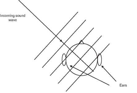
Figure 1. ITD arises from the difference in time of arrival of sound to the two ears, while IID is a result of sound attenuation by the head.

The second and equally important cue is the interaural intensity difference (IID), also known as interaural level difference (ILD), and is the result of the head being an obstacle that shadows the sound’s path to the eardrum. Since the head is a dense medium, a sound must diffract around the head to reach the far ear and its amplitude drops as a result. This effect is more perceptible when the wavelength of the sound is less than or comparable to the size of the head. As a result, the IID is more pronounced at high frequencies and provides complimentary information to the ITD. Other localization cues include the spectral cues and motion cues, which are useful in removing ambiguities associated with elevation discrimination when localization of both azimuth and elevation is required.

One of the earliest ITD processing models was proposed by Jeffress over 60 years ago (Jeffress, 1948), where he modeled the computation of ITD by having signals from the two ears propagating along delay lines in opposite directions and arriving at an array of coincidence detectors, each responding best to a particular ITD (Figure 2). This neural arrangement is analogous to a mathematical cross-correlation operation, with the delay between the signals given by the position of maximum correlation. Such neural computational circuits were later found in the owl’s brainstem (Konishi, 1992).

FIGURE 2

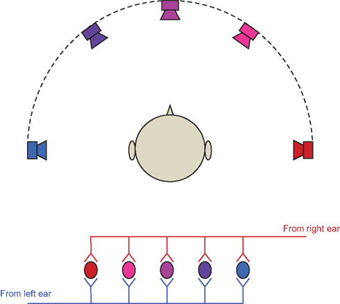
Figure 2. An illustration of Jeffress’ model. Each coincidence detector responses best to a particular ITD corresponding to sound arriving from a specific direction.

Localization systems are dominated by those based on ITD because time delay can be determined accurately, is relatively frequency independent (compared to IID), and its relationship with the source position can be most easily determined among all localization cues. Further, in many localization systems, the microphones are mounted on a plane or in free space so that no spectral cues or IIDs are available. Traditional ITD-based localization systems, whether using two microphones or a microphone array, often perform cross-correlation in software to determine the time delays between microphones (Huang et al., 1999, 2002; Julian et al., 2003, 2004). In systems with more than two microphones, these delays are combined using statistical methods, such as maximum likelihood or minimizing mean square error, to estimate the location of the source (Rabinkin et al., 1996; Svaizer et al., 1997). Alternatively, spatial temporal processing can be performed on the microphone array signals to compute the gradient of the sound field to obtain source direction (Clapp and Etienne-Cummings, 2002, 2004; Stanacevic and Cauwenberghs, 2005; Gore et al., 2010). While software implementations are more flexible, hardware implementations offer lower power consumption and guarantee real-time operation, which is especially important for sensor and robotic applications.

Some researchers have taken the bio-mimetic approach in an effort to build more human-like artificial systems. Subsequently, many of these systems employ biologically realistic strategies to perform sound localization. For instance, they use only two microphones mounted on a spherical head or manikin. A filter bank or Fourier Transform is often used to mimic the function of the biological cochlea, and the ITD and the IID in each band are then extracted. Some examples include the Cog project (Irie, 1995), the humanoid robot SIG (Nakadai et al., 2001; Okuno and Nakadai, 2003; Okuno et al., 2004), the robots used by Andersson and colleagues (Handzel et al., 2003; Andersson et al., 2004), and an audio-visual object localization system being developed by Schauer and Gross (2001).

Others have taken the challenge one step further by implementing some of these processing in analog VLSI (a-VLSI). The most notable was Lazzaro’s silicon model of sound localization (Lazzaro and Mead, 1989) based on Konishi’s owl model. In this implementation, the silicon cochleae decompose the incoming signals from the left and right ears into different frequency bands and convert the signals into spike trains. Cross-correlations are then performed on the spike trains using the silicon axons as delay lines and logic AND gates as coincident detectors, similar to the computation performed at the nucleus laminaris in the owls. The cross-correlation results are summed across frequency, and finally, a non-linear inhibition circuit is used to model the competition among inferior colliculus neurons, producing a neural map of ITD. A similar architecture was adopted by Bhadkamkar, who also implemented sound localization systems on chip but with limited success (Bhadkamkar and Fowler, 1993; Bhadkamkar, 1994). Both Lazzaro and Bhadkamkar’s work suffered from mismatch, particularly at the delay lines. Methods of extracting ITD without delay lines have been proposed by Shamma et al. (1989), van Schaik and Shamma (2003), and Grech et al. (2000, 2004). However, all these ITD extraction methods deviated somewhat from biology.

Once the ITDs from multiple bands are extracted they have to be processed to estimate the source location and several techniques can be used. In the first and simplest technique, it assumes the relationship between source location and ITD is known, e.g., if ITD = sin(θ), where θ is the azimuth angle of the source, then source location can be directly computed using the inverse function or a look-up table. Examples include (Huang et al., 1999; Julian et al., 2003).

The second method is a search strategy similar to the Nearest Neighbor Search, where the system searches through an entire range of discrete positions and the position resulting in the best match becomes the estimate. This is used by the ITD algorithm in Huang et al. (2002) and the IPD/IID algorithm in Handzel et al. (2003), Andersson et al. (2004). A more elaborated version is used by Grech et al. (2004) to localize sound in both azimuth and elevation. This method is more computationally intensive but offers greater flexibility and accuracy.

In the last method, the localization system is trained to learn the relationship between the sound features and source position, and the learning can be either supervised or unsupervised. In supervised learning, training data with known source positions are presented to the system, while in unsupervised learning, the source positions are not given explicitly but have to be determined by the system itself. This is usually achieved via the interaction of motion (head-turning) and sensing (both audition and vision). Examples of system which learns sound localization can be found in Irie (1995), Nakashima et al. (2002), Nakashima and Mukai (2005), Hornstein et al. (2006).

In this paper, we propose an ITD-based sound localization system that can be implemented in a-VLSI. The proposed system is biologically realistic as it uses only two sensors and it employs an a-VLSI cochlea model. Unlike some previous a-VLSI implementations, our solution requires no prior model of ITD and can be trained to localize sound in any environment. In addition, the training allows it to adapt to compensate for ITD variation across frequency and mismatch in circuit components.

This paper is organized as follows: the experimental setup is described in Sections “Experimental Setup” and “Materials and Methods,” we will introduce our approach to the localization problem, cumulating to a neuromorphic architecture supporting learning and adaptation; experimental results are presented next in Section “Results”; this is followed by a discussion in Sections “Discussion” and “Conclusion” will conclude the paper.

Experimental Setup

The experimental setup is shown in Figure 3. Two electret microphone capsules are mounted on opposite sides of a sphere 15 cm in diameter, made of foam. The microphone capsules measure 10 mm in diameter and are omnidirectional with a frequency range from 50 Hz to 12.5 kHz. The sphere itself is then fixed atop a robot, 15 cm from the ground. This sphere simulates the effect of head shadowing and diffraction introduced by the head, hence the recording from one microphone is not simply a time-delayed version of the other. Furthermore, because the head is mounted near the front of the robot, there are front-back asymmetries, which become evident in later sections. The microphone signals are amplified before being fed into the silicon cochlea chip, the AER EAR (Chan et al., 2007), and can be recorded and played back via a computer sound card.

FIGURE 3

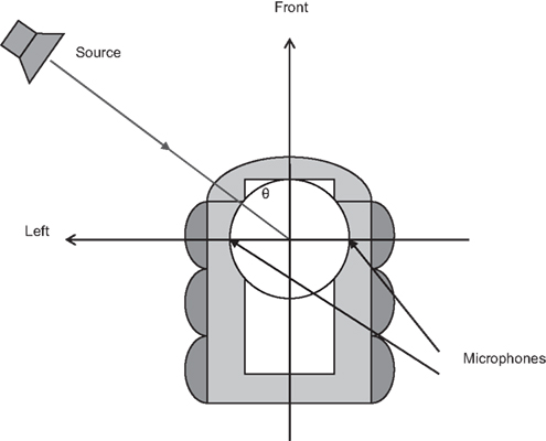
Figure 3. Localization setup. Two microphones are installed on opposite side of a 15 cm foam ball mounted on a 6-wheel robot. Azimuth = 0° at the front, 90° on the left, −90° on the right, and ±180° at the back.

We recorded the “head”-related impulse responses (IRs) of the microphones in response to a loudspeaker (Tannoy System 600A) at different azimuth positions in an “almost anechoic” environment. Although our “head” is a simple sphere, it is a good approximation in this case, since our system is ITD-based and pinna related spectral cues are minimal at the frequencies where ITD is thought to operate in humans (<3 kHz). The audio environment consists of a room in which the walls are fitted with sound absorbing material to minimize reflection with the only major reflection coming from the floor, which is covered with thick carpet. The Tannoy loudspeaker features concentric bass driver and tweeter unit to provide a single point source for all audio frequencies, and has a flat spectrum from 44 Hz to 20 kHz. It was placed at the same height as the sphere, 2.6 m from the center of the sphere, and the IRs were recorded at 10 steps. These IRs allow us to present any stimulus to the AER EAR to simulate a far-field source in an open environment for both learning and testing, from different directions, by simply convolving the source signal with the appropriate left and right IRs. This method also allows simulated automatic gain control to be applied to the signals before they enter the cochleae, which is required due to a limited dynamic range in our silicon cochlea.

Each of the two silicon cochleae in the AER EAR contain 32 sections and is tuned to cover the frequency range from 200 Hz to 10 kHz, logarithmically spaced. In the human cochlea the cut-off frequency of the low pass filter created by the inner hair cell (IHC) is around 1 kHz and significant phase locking cannot be expected for frequencies above 3 kHz. In biology, around 10 auditory nerves innervate a single IHC and many IHCs would cover a frequency range equivalent to the bandwidth of our silicon cochlea channels. To simulate many fibers innervating a single cochlear region with our AER cochlea, which has only one output address for this region, we have turned off the low-pass filtering in the IHC and used a high spike rate. At the same time any cochlear section with a best frequency above 3 kHz will not be used by the system, leaving us with 19 pairs of left and right cochlea channels for the current bias settings of the cochlea.

Each channel generates, on average, 6000 spikes per second when a 35 mV_rms sine wave is presented at the channel’s best frequency (BF). The leakage current at the integrate-and-fire neuron is adjusted to strike a balance between sensitivity and spontaneous spike rate. For demonstrative purposes, all processing after the cochlea has been performed in MATLAB.

Materials and Methods

Traditional Implementation

The block diagram of a commonly used bio-inspired algorithm for ITD-based sound localization (Lazzaro and Mead, 1989; Bhadkamkar and Fowler, 1993; Bhadkamkar, 1994; Lotz et al., 1999; Schauer and Paschke, 1999; Schauer and Gross, 2001) is shown in Figure 4. It is based on Jeffress’ model, where a pair of cochleae analyze the incoming sound and separate it into different frequency bands. Cross-correlation, typically implemented by delay lines and coincidence detectors, is then performed on the left and right outputs of each section, Y_{L i} and Y_{R i},

before being summed across frequency. The delay position with maximum correlation is selected using a winner-takes-all (WTA) circuit (Lazzaro et al., 1989; Indiveri et al., 2002) and becomes the estimate of the ITD.

If ITD is independent of frequency and determined by

where θ is the direction of the source (Figure 3), then direction can be computed from by applying the inverse function,

However, if the microphones are mounted on a head, the introduced diffraction will cause f(θ) to be frequency dependent, as shown in Figure 5. According to Kuhn (1977), at frequency less than 500 Hz, it can be approximated by a sine function, but becomes proportional to sin(θ) + θ as frequency increases above 1.5 kHz. Thus, different estimates will be given as the frequency of the source changes. The task is further complicated when implemented in a-VLSI as there will be mismatch in the delay lines at the cross-correlator, phase mismatch between the left and right cochleae, as well as mismatch in delay introduced by the signal conditioning circuits at the inputs of the cochleae.

FIGURE 4

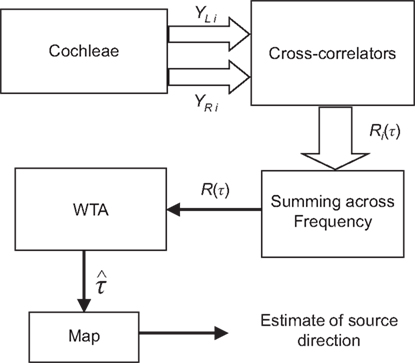
Figure 4. A commonly employed sound localization algorithm. A block arrow signifies a signal in multiple frequency bands. The cross-correlation results are summed across frequency without any adjustment for the frequency dependency of ITD.

FIGURE 5

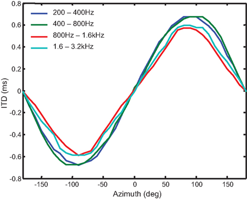
Figure 5. A plot of ITD vs. azimuth for two microphones mounted on opposite sides of the foam ball, for four different octave bands. The delay is larger at low frequencies, which is consistent with Kuhn’s model (Kuhn, 1977). Note that there are small front-back asymmetries (e.g., at 60º and 120º) at some frequencies due to the sphere being mounted near the front of the robot. Sound arriving from the back will experience more interference introduced by the robot’s body.

Mapping and Soft-WTA

The first and most intuitive solution to the ITD variation problem is to extract the delay in each band and individually map these delays to azimuth angles. They can then be averaged to obtain a global estimate. Since mapping is performed before the results are combined, the frequency dependency is corrected. A block diagram of the algorithm is shown in Figure 6.

FIGURE 6

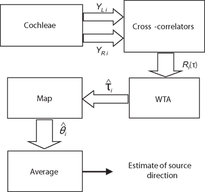
Figure 6. The first method to correct for ITD variation. For each band, the position of a single maximum is selected from the cross-correlation result using a WTA and mapped to azimuth position individually. These azimuth positions are then averaged to obtain the global estimate. The block arrows represent signals in multiple frequency bands.

While this algorithm works fine for noise inputs, it is less suitable for stimuli consisting of pure tones because the cross-correlation would result in more than one peak in some bands. If the wrong peak is picked, then in the best scenario, it is discarded (because it is physically impossible or is an outlier compared to the results from the other bands), resulting in some loss of information. In the worst case, however, it would generate a completely wrong estimate. This algorithm is also sensitive to noise and error introduced by mismatch at the WTA since only the delay corresponding to maximum correlation is extracted. Lastly, the implementation of a circuit capable of discarding outliers is not trivial. Therefore, we will investigate an alternative that is more robust and simpler to implement neuromorphically.

Instead of extracting only the global maximum in each band, it is more beneficial to retrieve all local maxima of significant magnitudes. In this way, even if the stimulus is a pure tone and the correlation result at the true time delay is not the global maximum, the true delay would still be passed on to subsequent stages rather than being discarded. This is accomplished by tuning the WTA. A typical WTA network is shown in Figure 7 and by adjusting the strength of the inhibition relative to that of the excitation, one can vary the selectivity. A weak to moderate global inhibition allows it to be used to implement the soft-max function, which selects not only the strongest but also those similar in strength (Indiveri and Delbruck, 2002). Figure 8 shows this system and Figure 9 shows the result of the application of a soft-WTA¹ (with the strength of inhibition equal to that of excitation) to a cross-correlation resulting from a pure tone stimulus. Both peaks are well-preserved.

FIGURE 7

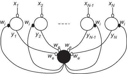
Figure 7. A winner-take-all network consists of neurons with excitatory and inhibitory synaptic connections. The global inhibitory neuron (in black) provides the negative feedback necessary for competition to occur. By adjusting the strength of the inhibition (W_i) relative to that of the excitation (W_e), one can vary the selectivity – more and more neurons go to zero as inhibition increases. (Adapted from (Indiveri and Delbruck, 2002)).

FIGURE 8

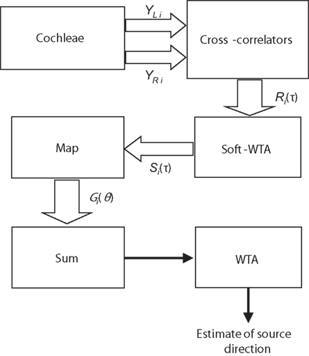
Figure 8. An improved algorithm using a Soft-WTA.

FIGURE 9

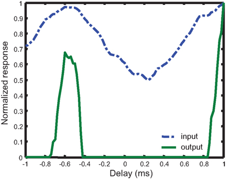
Figure 9. Application of soft-WTA to the result of cross-correlation. The stimulus is a 650 Hz pure tone with an ITD of approximately −0.6 ms. This ITD information would have been lost if a normal WTA is used, since there is a larger maximum at +1.0 ms.

Referring to Figure 8, for each frequency band, given the soft-WTA output S_i(τ), we can create a new function by mapping time (τ) to azimuth angle (θ) with the measured ITD function τ = f_i(θ),

This new function can be thought of as a measure of auditory activity at different bearing positions. Assuming there is only one source, the G_i(θ) in each band should produce a peak at the position of the source (even though there may be more than one peak if the signal is a mixture of pure tones). When the results are summed together, there will be one global maximum which gives us the correct estimate of the source direction:

Mapping as Matrix Multiplication

For the algorithm presented in Section “Mapping and Soft-WTA,” in each frequency band, the mapping essentially connects neurons representing the soft-WTA output at different delays, τ, with neurons representing auditory activity at different azimuth, θ. Since both time delay and angle are discrete, we can rewrite the WTA output as a vector S ∈ R^k and the activities at different azimuth as a vector G ∈ Rⁿ. The mapping can then be expressed as:

where W ∈ Rⁿ × R^k is a weight matrix. In each row, there will be only one “1” with all other entries being “0,” and the positions of the 1’s are given by the relationship between azimuth and ITD at that band. Thus, each neuron in G will receive spikes from exactly one neuron in S.

In biology, connections between neurons are never one-to-one. A typical neuron has dendritic trees that collect inputs from hundreds to thousands of other neurons, weighted differently depending on the synaptic strength. Such a rich network of interconnecting neurons allows computations involving hundreds of variables to be performed in parallel. Furthermore, it allows learning to take place gradually by making small incremental changes to synaptic strength, in contrast to the abrupt changes of updating a lookup table. With this mind, we generalize equation (7) and allow each element of W to take any value.

Now the question becomes: how do we determine W such that given the WTA output S, it can be transformed into G to represent activity in the auditory space? The solution can be found based on the gradient descent method.

In gradient descent, the goal is to find the point P such that f(P) is minimized. This is implemented by computing the gradient of f at the current position and move in the opposite direction, which gives the steepest rate of descent (Anderson, 1995). Mathematically, this can be expressed as:

where P_i is the current position, P_{i + 1} is the new position, and ε controls the rate of descent. In our case, given the input S and target T ∈ R^k, we define the error to be

and our aim is to find W which will minimize the square error function:

where t_i and g_i are the i-th elements of T and G, s_j is the j-th element of S, and W_ij is the element at the i-th row and j-th column of W. To determine the gradient, we take the partial derivative with respect to each element of W,

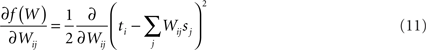
since this is the only term in the sum containing W_ij

So,

and our weight update rule² is

With a sufficiently small learning rate, ε, the error function will always converge to a local minimum. One of the elegant features of such an update rule is that learning can be performed online, i.e., the system can gradually adapt while in operation, as long as feedback is provided about the target position. This will allow us to implement a sound localization system that is continually trained by visual feedback, which will be the subject of a companion paper.

Figure 10 shows the complete block diagram of the final system. The mapping is replaced by a multiplication with a weight matrix. Such an operation is essential in artificial neural networks and has been implemented in VLSI with examples include (Morie, 1999; Serrano-Gotarredona and Linares-Barranco, 1999; Wang and Liu, 2006). Most implementations consist of an array of programmable synapses, with the weights stored in either digital or analog memory.

FIGURE 10

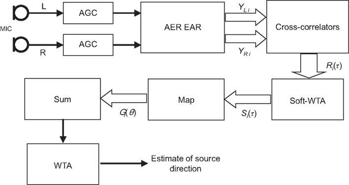
Figure 10. Block diagram of the final system. Mapping is replaced by matrix multiplication. S in each band is multiplied by a weight matrix to generate the activity map G. These frequency specific maps are then summed to produce the final estimate.

The complete system is simulated in MATLAB, except for the AER EAR, which was implemented in hardware. We use 101 delay positions (−1 to 1 ms with 20 μs resolution) and 61 azimuth angles (−90° to 90° with 3° step), resulting in weight matrices that are 61 × 101.

The weights are trained with band-limited noise stimuli under supervised learning. For each training example, we set the target T to be a Gaussian function centered at the expected position of the source, with σ = 25°. One of the advantages of choosing a Gaussian function instead of an impulse function is that it updates not only the weights going into the neuron representing the position of the source, but also those surrounding it. As a result, there is no need to provide training data at every source position and the system will be able to interpolate upon successful training. For simplicity, a fixed learning rate of 0.02 is used. While more complicated learning rate schedules can be used to speed up learning, we consider them outside the scope of this paper.

Results

After the weights have been trained, we are able to transform the soft-WTA outputs to a spatial map representing auditory activity. Figure 11 demonstrates this at one frequency channel. The outputs are essentially in a straight line, showing good correspondence between the actual and the perceived sound sources, with small imperfections at the larger azimuth positions. We repeat this process at a higher frequency channel with a different weight matrix, and again good results are shown in Figure 12.

FIGURE 11

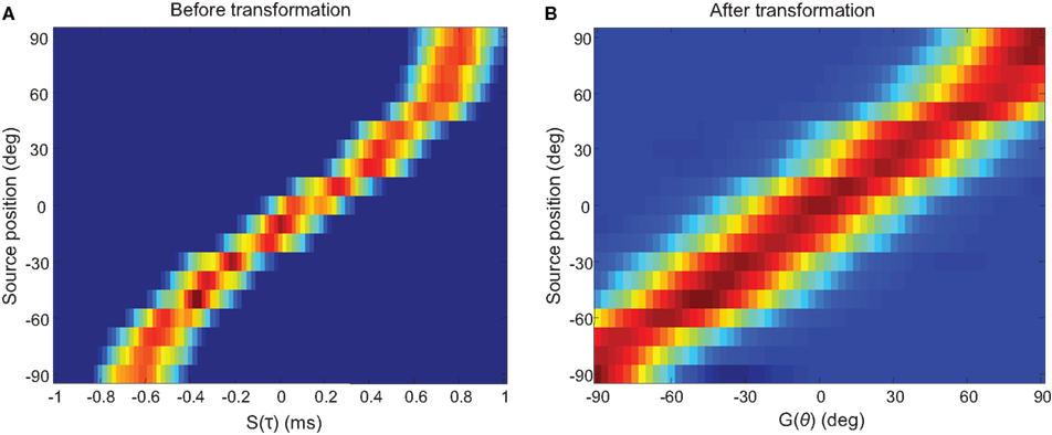
Figure 11. Before and after transformation at one channel with a best frequency (BF) of 340 Hz. (A) The soft-WTA output S, is transformed into (B) G, a representation of activity in auditory space for this frequency channel.

FIGURE 12

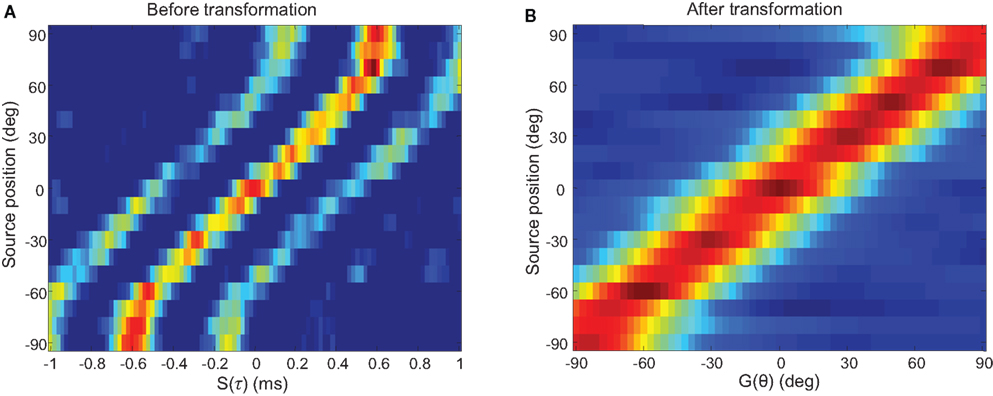
Figure 12. Before and after transformation at one channel with a BF of 2 kHz. (A) The soft-WTA output S, is transformed into (B) G, a representation of activity in auditory space for this frequency channel. The stimulus is band-limited noise centred at the BF. Unlike mapping, the transformation process is able to extract a unique source position from the positions of the three peaks in the cross-correlation result and there is no ambiguity.

Figure 13 shows how the error function f(W), in equation 10, reduces over time as the weights slowly adapt to the training data. The weights in the 2 kHz channel converge much slower than those in the 340 Hz channel. This is probably due to the gradual loss in phase-locking at the cochlea as frequency increases, resulting in more variation in the cross-correlation results, degrading the quality of the training data.

FIGURE 13

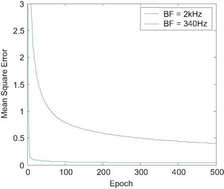
Figure 13. The mean square error as a function of epoch at two frequency channels with BF’s of 2 kHz and 340 Hz. It shows the weights adapt to slowly reduce the error. An epoch is a term used to describe the training of artificial neural network in which every training sample has been applied once.

Localization tests were performed after the weights had been trained. We tested the system with white noise (3 kHz bandwidth), a 400 Hz pure tone, and a 650 Hz pure tone, and the results are presented in Figures 14–16. 10 trials are performed at each source position and the average as well as the error of estimates is recorded. The front-back asymmetries that we saw in Figure 5, caused by the interference of the robot, are evident when the 650 Hz pure tone is played. Since the weights are trained with the source in front of the robot, the errors are large when the source comes from behind. The average RMS errors in the different ranges are presented in Table 1. The overall RMS error within the entire range is under 6º.

FIGURE 14

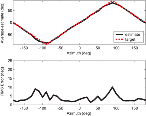
Figure 14. Localization result for a white noise stimulus, showing both the average estimate and RMS error at each position over 10 trials.

FIGURE 15

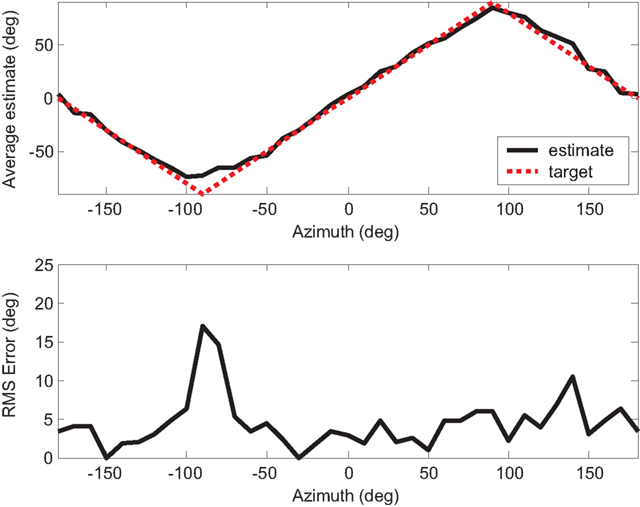
Figure 15. Localization result for a 400 Hz pure tone stimulus, showing both the average estimate and RMS error at each position over 10 trials.

FIGURE 16

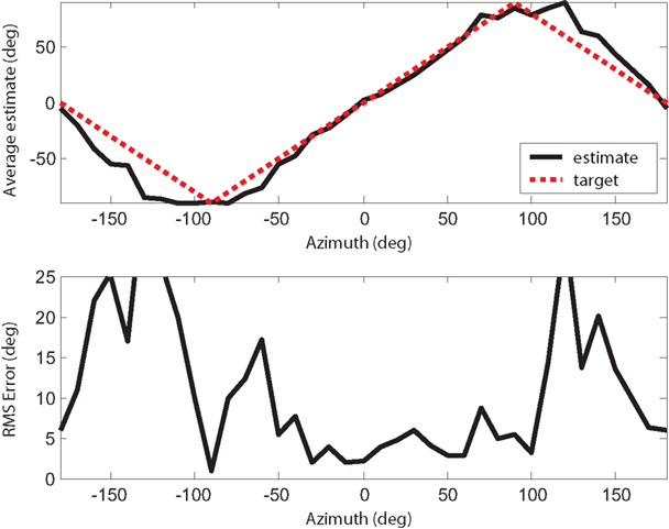
Figure 16. Localization result for a 650 Hz pure tone stimulus, showing both the average estimate and RMS error at each position over 10 trials.

TABLE 1

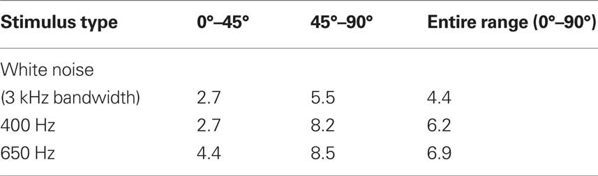
Table 1. RMS error for the three types of stimuli.

Discussion

In Table 2, we compare the performance of our system with other localization systems in which localization results are available or can be computed from published data. RMS errors are calculated manually from the average error and the standard deviation at each position, before they are combined across the two ranges, [0°, 45°] and [45°, 90°].

TABLE 2

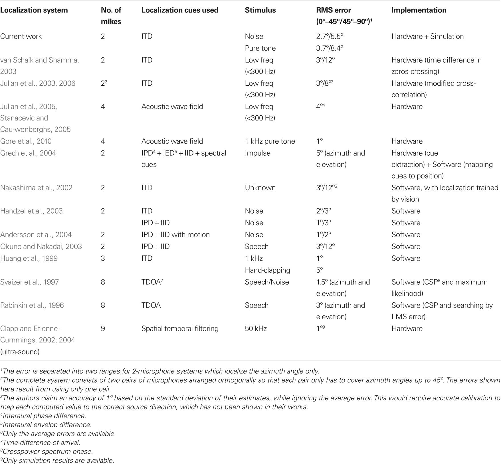
Table 2. Comparison with other sound localization systems.

The accuracy of our system is comparable with all the other 2-microphone hardware implementations (Julian et al., 2003; van Schaik and Shamma, 2003; Grech et al., 2004) and some software systems (Nakashima et al., 2002; Okuno and Nakadai, 2003). It can be seen that software systems generally offer better accuracy, with errors as low as 1° in the [0°, 45°] range, as computation can be performed in higher precision, at the expense of higher power consumption. For accurate 3-D source localization (i.e., azimuth, elevation and distance) in a reverberant and noisy environment, a microphone array has to be used.

Although our system only offers average performance in terms of accuracy, it is one of the most biologically realistic and the only one employing a pair of spiking cochleae. It is capable of localizing both white noise and pure tone sounds. This is in contrast to some existing systems which are tested with only one type of sound. Furthermore, our system is designed to adapt and learn during operation as long as feedback is provided. As a result, it is no longer necessary to accurately calibrate it to ensure good localization – instead the system will adapt and compensate for mismatch at the sensors and the processing circuitries. This is an important feature for both biological and robotic systems. However, for the system to adapt, feedback is needed with regards to the correct target position when the system encounters a new environment. In a companion paper, we will present a system that uses a silicon retina to provide visual feedback about the target positions in the visual field, which will be used to train the sound localization system.

Conclusion

An ITD-based neuromorphic sound localization system has been proposed. It uses the AER EAR as a front-end and unlike earlier attempts to implement neuromorphic sound localization systems in a-VLSI (Lazzaro and Mead, 1989; Bhadkamkar and Fowler, 1993; Bhadkamkar, 1994), by using a modular approach and processing each frequency channel individually, circuit mismatch and frequency dependent variations are overcome. The final system demonstrates the ability to reliably determine the azimuth position of the source for both pure tone and white noise sounds. In addition to the modest localization performance, this new architecture supports online learning, allowing the system to learn while in operation.

Conflict of Interest Statement

The authors declare that the research was conducted in the absence of any commercial or financial relationships that could be construed as a potential conflict of interest.

Footnotes

1. ^We use the term “soft-WTA” to describe any WTA network where the inhibition is weakened to allow more than one winner.
2. ^Gradient descent is used in the popular back-propagation algorithm to train multi-layers neural networks. The update rule is very similar, with the addition of an activation function (Anderson, 1995; Russell and Norvig, 1995).

References

Anderson, J. A. (1995). Gradient Descent Algorithms, An Introduction to Neural Networks. Cambridge, MA: MIT Press, 239–279.

Andersson, S. B., Handzel, A. A., Shah, V., and Krishnaprasad, P. S. (2004). Robot phonotaxis with dynamic sound localization. IEEE Int. Conf. Robot. Autom. 5, 4833–4838.

Bhadkamkar, N. A. (1994). Binaural source localizer chip using subthreshold analog CMOS. IEEE Int. Conf. Neural Netw. 3, 1866–1870.

Bhadkamkar, N. A., and Fowler, B. (1993). Sound localization system based on biological analogy. IEEE Int. Conf. Neural Netw. 3, 1902–1907.

CrossRef Full Text

Chan, V., Liu, S.-C., and van Schaik, A. (2007). AER EAR: a matched silicon cochlea pair with address event representation interface. IEEE Trans. Circuits Syst. I: Regul. Pap. 54, 48–59.

CrossRef Full Text

Clapp, M. A., and Etienne-Cummings, R. (2002). Ultrasonic bearing estimation using a MEMS microphone array and spatiotemporal filters. IEEE Int. Symp. Circuits Syst. 1, 661–664.

Clapp, M. A., and Etienne-Cummings, R. (2004). Bearing angle estimation for sonar micro-array using analog VLSI spatiotemporal processing. IEEE Int. Symp. Circuits Syst. 4, 884–887.

Grech, I., Micallef, J., and Vladimirova, T. (2000). Low-voltage, SC TDM correlator for the extraction of time delay. IEEE Int. Conf. Electron. Circuits Syst. 1, 112–115.

Grech, I., Micallef, J., and Vladimirova, T. (2004). Analog CMOS chipset for a 2-D sound localization system. Analog Integr. Circuits Signal Process. 41, 167–184.

CrossRef Full Text

Gore, A., Fazel, A., and Chakrabartty, S. (2010). Far-field acoustic source localization and bearing estimation using σΔ learners. IEEE Trans. Circuits Syst. I: Regul. Pap. 57, 783–792.

CrossRef Full Text

Handzel, A. A., Andersson, S. B., Gebremichael, M., and Krishnaprasad, P. S. (2003). A biomimetic apparatus for sound-source localization. IEEE Conf. Decis. Control 6, 5879–5884.

Hornstein, J., Lopes, M., Santos-Victor, J., and Lacerda, F. (2006). Sound localization for humanoid robots – Building audio-motor maps based on the HRTF. IEEE/RSJ Int. Conf. Intell. Robots Syst. 1170–1176.

Huang, J., Kume, K., Saji, A., Nishihashi, M., Watanabe, T., and Martens, W. L. (2002). Robotic spatial sound localization and its 3-D sound human interface. Int. Symp. Cyber Worlds 191–197.

Huang, J., Supaongprapa, T., Terakura, I., Wang, F., Ohnishi, N., and Sugie, N. (1999). A model-based sound localization system and its application to robot navigation. Rob. Auton. Syst. 27, 199–209.

CrossRef Full Text

Indiveri, G., and Delbruck, T. (2002). “Current-mode circuits,” in Analog VLSI: Circuits and Principles, eds S.-C. Liu, J. Kramer, G. Indiveri, T. Delbrũck, and R. Douglas (Cambridge, MA: MIT Press), 145–175.

Irie, R. E. (1995). Robust Sound Localization: An Application of an Auditory Perception System for a Humanoid Robot. Master Thesis, Department of Electrical Engineering and Computer Science, Massachusetts Institute of Technology, Cambridge, MA.

Jeffress, L. A. (1948). A place theory of sound localization. J. Comp. Physiol. Psychol. 41, 35–39.

Pubmed Abstract | Pubmed Full Text | CrossRef Full Text

Julian, P., Andreou, A. G., Mandolesi, P., and Goldberg, D. (2003). A low-power CMOS integrated circuit for bearing estimation. IEEE Int. Symp. Circuits Syst. 5, 305–308.

Julian, P., Andreou, A. G., Riddle, L., Shamma, S., Goldberg, D.H., and Cauwenberghs, G. (2004). A comparative study of sound localization algorithms for energy aware sensor network nodes. IEEE Trans. Circuits Syst. I: Regul. Pap. 51, 640–648.

CrossRef Full Text

Julian, P., Andreou, A. G., and Shamma, S. (2005). Field test results for low power bearing estimator sensor nodes. IEEE Int. Symp. Circuits Syst. 5, 4205–4208.

CrossRef Full Text

Julian, P., Andreou, A. G., and Goldberg, D. H. (2006). A low-power correlation-derivative CMOS VLSI circuit for bearing estimation. IEEE Trans. VLSI Syst. 14, 207–212.

CrossRef Full Text

Konishi, M. (1992). The neural algorithm for sound localization in the owl. Harvey Lect. Ser. 86, 47–64.

Kuhn, G. F. (1977). Model for the interaural time differences in the azimuthal plane. J. Acoust. Soc. Am. 62, 157–167.

CrossRef Full Text

Lazzaro, J., and Mead, C. A. (1989). A silicon model of auditory localization. Neural. Comput. 1, 47–57.

CrossRef Full Text

Lazzaro, J., Ryckebusch, S., Mahowald, M. A., and Mead, C. A. (1989). Winner-take-all networks of O(n) complexity. Neural Inf. Process. Syst. Conf. 1, 703–711.

Lotz, K., Boloni, L., Roska, T., and Hamori, J. (1999). Hyperacuity in time: a CNN model of a time-coding pathway of sound localization. IEEE Trans. Circuits Syst. I: Fundam. Theory Appl. 46, 994–1002.

CrossRef Full Text

Morie, T. (1999). “Analog VLSI implementation of self-learning neural networks”, in Learning On Silicon, eds. G. Cauwenberghs and M. A. Bayoumi (Boston, Dordrecht, London: Kluwer Academic Publishers), 213–242.

Nakadai, K., Okuno, H. G., and Kitano, H. (2001). Epipolar geometry based sound localization and extraction for humanoid audition. IEEE/RSJ Int. Conf. Intell. Robots Syst. 3, 1395–1401.

Nakashima, H., and Mukai, T. (2005). 3D sound source localization system based on learning of binaural hearing. IEEE Int. Conf. Syst. Man Cybern. 4, 3534–3539.

Nakashima, H., Mukai, T., and Ohnishi, N. (2002). Self-organization of a sound source localization robot by perceptual cycle. Int. Conf. Neural Inf. Process. 2, 834–838.

Okuno, H. G., and Nakadai, K. (2003). Real-time sound source localization and separation based on active audio-visual integration. Int. Work Conf. Artif. Nat. Neural Netw. 1, 118–125.

Okuno, H. G., Nakadai, K., Laourens, T., and Kitano, H. (2004). Sound and visual tracking for humanoid robot. Appl. Intell. 20, 253–266.

CrossRef Full Text

Rabinkin, D. V., Renomeron, R. J., Dahl, A., French, J., and Bianchi, M. H. (1996). A DSP implementation of source location using microphone arrays. J. Acoust. Soc. Am. 99, 2503–2529.

CrossRef Full Text

Russell, S., and Norvig, P. (1995). Artificial Intelligence: A Modern Approach. Upper Saddle River, NJ: Prentice Hall, 578–584.

Schauer, C., and Gross, H.-M. (2001). A model of horizontal 360° object localization based on binaural hearing and monocular vision. Int. Conf. Artif. Neural Netw. 2130, 1141–1146.

Schauer, C., and Paschke, P. (1999). A spike-based model of binaural sound localization. Int. J. Neural Syst. 9, 447–452.

Pubmed Abstract | Pubmed Full Text | CrossRef Full Text

Serrano-Gotarredona, T., and Linares-Barranco, B. (1999). “ART1 and ARTMAP VLSI circuit implementation,” in Learning On Silicon, eds G. Cauwenberghs and M. A. Bayoumi (Boston, Dordrecht, London: Kluwer Academic Publishers), 163–191.

Shamma, S., Shen, N., and Gopalaswamy, P. (1989). Stereausis: binaural processing without neural delays. J. Acoust. Soc. Am. 86, 989–1006.

Pubmed Abstract | Pubmed Full Text | CrossRef Full Text

Stanacevic, M., and Cauwenberghs, G. (2005). Micropower gradient flow acoustic localizer. IEEE Trans. Circuits Syst. I: Regul. Pap. 52, 2148–2157.

CrossRef Full Text

Svaizer, P., Matassoni, M., and Omologo, M. (1997). Acoustic source location in a three-dimensional space using crosspower spectrum phase. IEEE Int. Conf. Acoust. Speech Signal Process. 1, 231–234.

van Schaik, A., and Shamma, S. (2003). A neuromorphic sound localizer for a smart MEMS system. IEEE Int. Symp. Circuits Syst. 4, 864–867.

Wang, X., and Liu, S.-C. (2006). Programmable synaptic weights for an aVLSI network of spiking neurons. IEEE International Symposium on Circuits and Systems, 4531–4534.