Positive Temporal Dependence of the Biological Clock Implies Hyperbolic Discounting

Temporal preferences of animals and humans often exhibit inconsistencies, whereby an earlier, smaller reward may be preferred when it occurs immediately but not when it is delayed. Such choices reflect hyperbolic discounting of future rewards, rather than the exponential discounting required for temporal consistency. Simultaneously, however, evidence has emerged that suggests that animals and humans have an internal representation of time that often differs from the calendar time used in detection of temporal inconsistencies. Here, we prove that temporal inconsistencies emerge if fixed durations in calendar time are experienced as positively related (positive quadrant dependent). Hence, what are time-consistent choices within the time framework of the decision maker appear as time-inconsistent to an outsider who analyzes choices in calendar time. As the biological clock becomes more variable, the fit of the hyperbolic discounting model improves. A recent alternative explanation for temporal choice inconsistencies builds on persistent under-estimation of the length of distant time intervals. By increasing the expected speed of our stochastic biological clock for time farther into the future, we can emulate this explanation. Ours is therefore an encompassing theoretical framework that predicts context-dependent degrees of intertemporal choice inconsistencies, to the extent that context can generate changes in autocorrelation, variability, and expected speed of the biological clock. Our finding should lead to novel experiments that will clarify the role of time perception in impulsivity, with critical implications for, among others, our understanding of aging, drug abuse, and pathological gambling.

1 Introduction

Suppose we are asked to choose between $10 now or $11 tomorrow. We may prefer the $10 immediately rather than the $11 received after a day. However, if we are offered to choose between $10 to be received after 364 days, or $11 after 365 days, we often prefer to wait the additional day for the extra dollar. After waiting 364 days, the latter choice becomes one between an immediate $10 or $11 tomorrow. Now we would want to reverse it, asking for the $10 immediately, rather than waiting the extra day we seemed to have been willing to accept in the past. This time inconsistency can be modeled using hyperbolic discounting of future rewards (Laibson, 1997). To avoid inconsistencies, rewards should be discounted exponentially over time (Sutton and Barto, 1998).

Here, we conjecture that hyperbolic discounting has a rational explanation, based on the generally accepted principal that the animal and human biological clocks tick at a different rate from the calendar clock. Animals and humans are indeed known to maintain an internal representation of time that differs from standard calendar time and whose properties change with time scale, from microseconds up to years, with representations of (calendar) time at larger scales showing the highest variability (Buonomano, 2007). In humans, drugs (Meck, 1998; Wittmann et al., 2007), and age (Mischel et al., 1989), among other things, are known to influence time perception. The neurobiological mechanism behind the biological clock has recently become a topic of intense study (Buhusi and Meck, 2005).

We start from the preposition that discounting is exponential, as required for time-consistent choice. At the same time, we posit that the internal representation of time (under which discounting occurs) varies stochastically (randomly) from calendar time. This is illustrated in Figure 1: two events at times 0 and Δ in calendar are experienced to occur at t₀ = F(0) and t_Δ = F(Δ) in biological time, where F is some stochastic (random) transformation F.

FIGURE 1

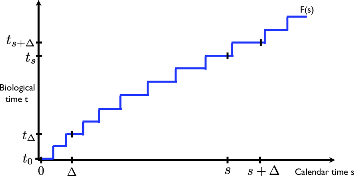
Figure 1. The calendar time and biological time evolve at different rates. Two equal intervals (0, Δ) and (s, s + Δ) in calendar time (horizontal axis) translate into unequal intervals (t₀, t_Δ) and (t_s, t_{s + Δ}) in biological time (vertical axis). The function F(•) depicts one possible realization of the (stochastic) transformation from calendar to biological time.

Now consider two events at a later time s and s + Δ, separated by the same amount of (calendar time) delay Δ. The times s and s + Δ are transformed to t_s = F(s) and t_{s + Δ} = F(s + Δ) in biological time. Although the delay between the pair of events is the same in calendar time, the corresponding delay between the events in biological time, t_Δ − t₀ and t_{s + Δ} − t_s are generally different.

We assume that the biological clock is positive quadrant dependent (Esary et al., 1967). Intuitively, this means that if t_s is small, the chance increases that the subsequent interval t_Δ − t_s is small too. It implies positive autocorrelation, i.e., cov(t_s, t_{s + Δ} − t_s) > 0. And crucially, it implies that discount factors are positive autocorrelated: cov(exp(−t_s), exp(−(t_{s + Δ} − t_s))) > 0. We also assume that increments in biological time are stationary: the distribution of time changes does not depend on when they occur; the distribution of t_Δ − t₀ is the same as that of t_{s + Δ} − t_s. The following theorem states the main result.

Theorem: Positive Dependence in Biological Time Implies Temporal Choice Inconsistency

The rigorous proof of the theorem is provided in the Section “Appendix,” that the reader is encouraged to peruse. Here we aim to provide the intuition with a simple numerical example. We envisage delivery of $1 now or K dollars at Δ (a point in calendar time). K is to be chosen so that there is indifference. We then compare delivery of $1 at s = 2 with delivery of K dollars at s = 2 + Δ.

The biological clock is as follows. Either s feels like it takes 1 unit of (biological) time, or it takes 3 units, with an average of 2 units. Δ is on average half the length; it feels either short (0.5 units) or long (1.5), with an average of 1 unit.

The biological clock is positive quadrant dependent. We will make the dependence perfect, to simplify the argument. When s feels like it takes 1 unit, the subsequent Δ will take 0.5 unit; when s feels long (2 units), the subsequent Δ is long as well, at 1.5 units.

As mentioned, K is set so that there is indifference between getting $1 now and K dollars at Δ. Today’s value of K is 0.5^* exp(−0.5) + 0.5^* exp(−1.5)^* K, because with 50% probability, delivery is felt like taking place in 0.5 units of (biological) time, and with 50% chance, it feels like it takes place 1.5 time units in the future. We set K so that today’s value equals $1. So, K = 2/(exp(−0.5) + exp(−1.5)) = 2.411.

Essentially, K is set so that the gain of having to wait a short time (only 0.5 units of biological time) is offset by the loss in value for having to wait a long time (1.5 units). The former gain (relative to today’s $1) is 2.411^* exp(−0.5) − 1 = 0.462, or 46.2%; the latter loss equals 1 − 2.411^* exp(−1.5) = (1 − 0.538) = 46.2%. The gains and losses offset.

As for delivery of K at s + Δ, notice that, while the gain and loss from waiting an extra Δ beyond s have equal probability of occurring, they are discounted differently. The gain occurs when s = 2 arrives early under the biological clock (1 unit); this is weighted more heavily, because it is discounted with only exp(−1); its weighted value is exp(−1)^* 1.462 = 0.538. The loss when s = 2 arrives late (3 units under the biological clock) is weighted less, because it occurs farther in time; it is discounted with exp(−3); the weighted value in that case is exp(−3)^* 0.538 = 0.027. In expectation, the value of receiving K at s + Δ equals (0.538 + 0.027)/2 = 0.283.

Compare this to getting $1 at s = 2. There is no loss or gain (one always gets $1). With 50% probability, the dollar arrives early (1 unit in biological time), and its discounted value is exp(−1) = 0.368, and with 50% chance the dollar arrives late (3 units under the biological clock), and its discounted value is exp(−3) = 0.050. In expectation, the value equals (0.368 + 0.050)/2 = 0.209. This is strictly less than the value of getting K delayed (0.283).

Hence, while K was set to be indifferent between receiving $1 now and K dollars at Δ, the promise of K at s + Δ is worth more than getting $1 at s.

The astute reader will have noticed that the positive dependence of the biological clock is not really needed to get time inconsistencies. They occur also with negative dependence. However, with positive dependence, the decision maker will always prefer to wait when comparing options in the future for which she is indifferent now. That is, she looks more patient when deciding about payoffs in the future. This is the classical time inconsistency that has led to modeling of intertemporal choice using hyperbolic discounting. With negative dependence, the decision maker looks more patient in the immediate future than when considering options in the far future.

2 Simulations

We now illustrate that hyperbolic discounting provides a good fit to the choices resulting from positive temporal dependence of biological time. To model biological time, we choose the lognormal distribution (Jaynes, 2003), which has a continuous positive support. Under the biological clock, any two time increments, such as t_Δ − t₀ and t_{s + Δ} − t_s, are jointly lognormal. When the time increments are positively correlated, they will also be positive quadrant dependent (this follows from Pitt, 1983), and hence, the corresponding discount factors will be positively correlated as well.

To make the example concrete, consider the choice between a payoff of 1 at time 0, and 1 + K at a delay (in calendar time) of Δ = 0.5. We compare this to a pair of later options equally distanced in calendar time, at s = 2 and at s + Δ = 2.5. In biological time, these events are at t₀ = 0 and t_Δ for the first pair, t_s and t_{s + Δ}, for the second pair. The time of payoff delivery under the biological clock is a random variable.

We obtain the values of the options by Monte Carlo sampling. To generate the samples, we consider n increments in biological time, 𝝉₁,…, 𝝉_n, that correspond to time increments of 0.5 units in calendar time. The n increments in biological time are drawn from a multivariate lognormal distribution with common mean 0.5 and unit variance. The correlations between the increments are positive, but decrease exponentially as they are farther apart in time. We encode the correlation structure as a covariance matrix with diagonals equal to 1, and covariances equal to ρ, ρ²,…, ρ^{n − 1} in the off-diagonal spots (see Appendix). We obtain instances in biological time by adding increments: t_Δ = 𝝉₁, and These formulae reflect the fact that the biological expiration time of the delayed early option occurs after one increment, while the two later options mature after four and five increments, respectively.

For the first option pair, the value of the immediate option is 1, and the option with payoff at (calendar time) Δ = 0.5, is valued at assuming a unit discount rate (in biological time). Monte Carlo analysis based on N(=10⁶) samples of t_Δ estimates this to be For K = 0.78, we find that i.e., the decision maker is approximately indifferent between immediate delivery of $1 and a payoff of $1.78 after a delay of Δ = 0.5 units of calendar time.

For the pair of options at the more distant future, the values of the early and later options are estimated to remain approximately equal when time increments are independent, i.e., ρ = 0 When time increments are positively correlated, i.e., ρ > 0, the later option is valued more highly, in accordance with our Theorem. For example, when ρ = 0.5, the early option has value and the later option has value 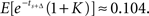So the decision maker prefers to wait to receive $1.78 later, while he was indifferent between an immediate $1 and $1.78 after an equally long delay of Δ = 0.5. We thus have obtained a temporal inconsistency.

We can obtain a discounting curve by evaluating payoffs at various delays, as in the previous example. We generated n(=10) increments, 𝝉₁,…, 𝝉_n, of length Δ = 0.5. The time indicated by the biological clock at calendar time s is given by The value of a payoff of $1 at time 0 is 1, and at (calendar) time s is (we continue to use a unit discount rate.) The values obtained for each point in calendar time can then be compared to valuation with hyperbolic discounting (in calendar time), assuming a discount factor is 1/(1 + ks). We find the best-fitting value of k by minimizing the squared error between the theoretical values under the hyperbolic function, and that generated by our Monte Carlo procedure. Similarly, we can also obtain a comparison with valuation (in calendar time) assuming exponential discounting, where the discount factor equals e^−δs. The discount rate δ is also obtained by minimizing the squared error.

We are interested, in particular, in the effect of the correlation parameter ρ of the biological clock on the shape of the discounting curve. When autocorrelation equals zero (ρ = 0), the discounting curve is pretty much exponential, as shown in Figure 2 (Top). The best-fitting exponential curve has δ = 0.3; this differs from the true discount rate (1) because the latter only applies to biological time. The hyperbolic curve has k = 2.75, but its fit is worse. Figure 2 (Bottom) illustrates how, when the autocorrelations are very high (ρ = 0.97), hyperbolic discounting provides the better fit. The best-fitting exponential discount rate equals δ = 0.45, and the hyperbolic discount rate is estimated at k = 1.75.

FIGURE 2

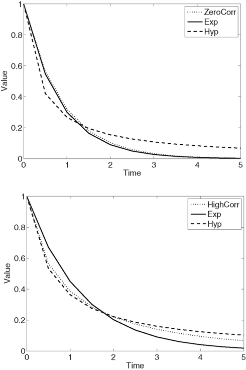
Figure 2. (Top) No autocorrelation of biological time (ρ = 0). The discounting curve in biological time is exponential with discount rate equal to 1. It generates the dotted discounting curve in calendar time (“ZeroCorr”). The best exponential (“Exp”) fit in calendar time produces a discount rate of 0.30, and the best hyperbolic fit (“Hyp”) has a discount rate equal to 2.75. (Bottom) Very high autocorrelation of biological time (ρ = 0.97). The discounting curve in biological time is exponential with discount rate equal to 1. It generates the dotted discounting curve in calendar time (“HighCorr”). The best exponential (“Exp”) fit in calendar time produces a discount rate of 0.45, and the best hyperbolic fit (“Hyp”) in calendar time has discount rate equal to 1.75.

Variability in the mapping from calendar to biological time also plays a role. In the limit, when the biological clock is accurate (i.e., the mapping is deterministic, and, because we assume a constant speed for the biological clock, linear), we of course obtain exponential discounting in calendar time. Section A3 in Appendix shows how variability induces increased convexity in the discounting curve.

3 Discussion

Time inconsistencies, like the ones that led to modeling time preferences with hyperbolic discounting, arise when the biological clock advances randomly in calendar time, and increments in biological time are positively dependent. When measured in calendar time, discounting becomes increasingly hyperbolic as the biological clock becomes more highly correlated and more variable.

Prior to our result, hyperbolic discounting emerged in a normative (i.e., fully rational) model because discount rates were assumed to be stochastic (Farmer and Geneakopolos, 2009). Our rational explanation of hyperbolic discounting does not rely on random discounting, but on randomness in the transformation between calendar time (which determines payoff times) and biological time (which is relevant for decision making). The two explanations can be shown to be related mathematically, but they are biologically very different. Specifically, stochastic time perception is biologically plausible, while stochastic discounting is rarely considered outside the arcane world of mathematical finance. An exception is Skog (1997).

Other rational explanations of hyperbolic discounting focus on specific forms of uncertainty about the ability of the payer to deliver the future payment (because he is bankrupted) or of the payee to receive it (because she may have deceased beforehand). When the hazard rate is stochastic, the apparent discount rate can be shown to become stochastic (see Sozou, 1998; Azfar, 1999; Sozou and Seymour, 2003). However, payment uncertainty cannot provide a comprehensive explanation. In particular, it fails to explain hyperbolic discounting in experiments where design precludes bankruptcy and where the time horizon is too short for significant effects from sudden inability of the payee to take delivery (e.g., Kable and Glimcher, 2007).

Our explanation of hyperbolic discounting assumes that discounting is exponential in biological time. Consistent with this, temporal discounting has empirically been shown to have an exponential form when subjective estimates of time elapsed are taken into account (Zauberman et al., 2009). Other work has shown that discounting is hyperbolic if subjects perceive realizations of future events to be uncertain (Dasgupta and Maskin, 2005).

The importance of perceived time in discounting has been pointed out before (Kim and Zauberman, 2009; Nakahara and Kaveri, 2010), but because random time changes were never considered, some type of misperception had to be invoked to generate hyperbolic discounting and the associated choice inconsistencies. Specifically, in Kim and Zauberman (2009), Nakahara and Kaveri (2010), the mapping from calendar to biological time is concave, so that increments farther in calendar time are expected (under the biological clock) to become shorter, inconsistent with the actual experience once the future arrives. In contrast, in our case, the speed of the biological clock is in tune with the calendar time, on average. Our approach relies on variability in the estimates.

Still, we can emulate the misperception of Kim and Zauberman (2009), Nakahara and Kaveri (2010) by increasing the expected speed of the biological clock for time farther into the future, or equivalently, decreasing the drift in the mapping from calendar to biological time. This generates concavity in the (random) mapping from calendar to biological time, and hyperbolic discounting adequately captures the resulting intertemporal choices; see Section A4 in Appendix. Positive dependence in the biological clock is no longer needed; nor is variability. As such, our framework encompasses explanations that rely on concavity in the mapping from calendar to biological time.

Stochasticity in time perception has long been accepted in psychology. Gibbon et al. (1984), e.g., uses a random clock process to explain response accuracy in animal timing tasks. Consideration of temporal dependence of the biological clock is novel, however, and may elucidate timing anomalies that an independent clock cannot explain (Machado and Keen, 1999). Positive temporal correlation in the internal clock is neurobiologically plausible; it may be supported by the positive autocorrelations recently discovered in human brain activity oscillations, displaying slow decreases even over thousands of cycles (Linkenkaer-Hansen et al., 2001, 2004), not unlike those generated by fractional Brownian motions (Mandelbrot and Van Ness, 1968). It is unknown to what extent this generalizes to longer time horizons, however.

Our theoretical framework provides a potentially unifying account for recorded time preferences. This is fortunate, because hyperbolic discounting is known to not be universal, with the shape (and level) of discounting changing with context (Scholten and Read, 2010). Context-dependence is consistent with our theory, which implies exponential discounting when the speed of the internal clock is expected to be constant, and the relation between calendar time and biological time accurate, or increments in biological time uncorrelated. Hyperbolic discounting emerges when the biological clock exhibits temporal dependence, or when its speed is expected to decrease in the more distant future. Future research should clarify which features of the biological clock can account for the observed context-dependence of discounting. In Scholten and Read (2010), intertemporal preferences were observed to be different depending on whether a time interval is divided up, or time is extended by adding intervals. In principle, our theory could accommodate such differences, but it may require the biological clock to not be self-similar (Mandelbrot and Van Ness, 1968); that is, its temporal properties may have to change as one moves from coarser to finer sub-divisions of time.

Our theorem provides a new, unifying framework to study time perception and how it relates to impulsivity in temporal decision making (Wittmann and Paulus, 2008). Our linking the phenomena of biological time and intertemporal discounting should lead to novel studies of the symptoms and causes of many disorders involving anomalous time perception, such as attention-deficit hyperactivity syndrome, borderline personality disorder, anxiety disorder, and schizophrenia.

Conflict of Interest Statement

The authors declare that the research was conducted in the absence of any commercial or financial relationships that could be construed as a potential conflict of interest.

Acknowledgments

We would like to thank Peter Dayan for useful comments and for pointing out a mistake in the previous version of our proof, and to the reviewers for their insightful comments. The U.S. National Science Foundation provided funding under grant SES-0616431.

References

Azfar, O. (1999). Rationalizing hyperbolic discounting. Am. Econ. Rev. 38, 245–252.

Buhusi, C. V., and Meck, W. H. (2005). What makes us tick? Functional and neural mechanisms of interval timing. Nat. Rev. Neurosci. 6, 755–765.

Pubmed Abstract | Pubmed Full Text

Buonomano, D. V. (2007). The biology of time across different scales. Nat. Chem. Biol. 3, 594–597.

Pubmed Abstract | Pubmed Full Text

Dasgupta, P., and Maskin, E. (2005). Uncertainty and hyperbolic discounting. Am. Econ. Rev. 95, 1290–1299.

Esary, J. D., Proschan, F., and Walkup, D. W. (1967). Association of random variables, with applications. Ann. Math. Stat. 38, 1466–1474.

Farmer, J. D., and Geneakopolos, J. (2009). Hyperbolic Discounting is Rational: Valuing the far Future with Uncertain Discount Rates. Cowles Foundation Discussion paper no. 1719, New Haven: Yale University. http://papers.ssrn.com/sol3/papers.cfm?abstract_id=1448811

Gibbon, J., Church, R. M., and Meck, W. H. (1984). Scalar timing in memory. Ann. N. Y. Acad. Sci. 423, 52–77.

Pubmed Abstract | Pubmed Full Text

Jaynes, E. T. (2003). Probability Theory: The Logic of Science, Vol. 1. Cambridge, UK: Cambridge University Press.

Kable, J. W., and Glimcher, P. W. (2007). The neural correlates of subjective value during intertemporal choice. Nat. Neurosci. 10, 1625–1633.

Pubmed Abstract | Pubmed Full Text

Kim, B. K., and Zauberman, G. (2009). Perception of anticipatory time in temporal discounting. J. Neurosci. Psychol. Econ. 2, 91–101.

Laibson, D. (1997). Golden eggs and hyperbolic discounting. Q. J. Econ. 112, 443–447.

Linkenkaer-Hansen, K., Nikouline, V. V., Palva, J. M., and Ilmoniemi, R. J. (2001). Long-range temporal correlations and scaling behavior in human brain oscillations. J. Neurosci. 21, 1370–1377.

Pubmed Abstract | Pubmed Full Text

Linkenkaer-Hansen, K., Nikulin, V. V., Palva, J. M., Kaila, K., and Ilmoniemi, R. J. (2004). Stimulus-induced change in long-range temporal correlations and scaling behaviour of sensorimotor oscillations. Eur. J. Neurosci. 19, 203–218.

Pubmed Abstract | Pubmed Full Text

Machado, A., and Keen, R. (1999). Learning to time (LET) or scalar expectancy theory (SET)? A critical test of two models of timing. Psychol. Sci. 10, 285–290.

Mandelbrot, B. B., and Van Ness, J. W. (1968). Fractional Brownian motions, fractional noises and applications. SIA Rev. 10, 422–437.

CrossRef Full Text

Meck, W. H. (1998). Neuropharmacology of timing and time perception. Cogn. Brain Res. 6, 233–233.

Mischel, W., Shoda, Y., and Rodriguez, M. L. (1989). Delay of gratification in children. Science 244, 933–938.

Pubmed Abstract | Pubmed Full Text | CrossRef Full Text

Nakahara, H., and Kaveri, S. (2010). Internal-time temporal difference model for neural value-based decision making. Neural. Comput. 22, 3062–3106.

Pubmed Abstract | Pubmed Full Text

Pitt, L. (1983). Positively correlated normal variables are associated. Ann. Probab. 10, 496–499.

CrossRef Full Text

Scholten, M., and Read, D. (2010). The psychology of intertemporal tradeoffs. Psychol. Rev. 117, 925–944.

Pubmed Abstract | Pubmed Full Text

Skog, O. (1997). The strength of weak will. Ration. Soc. 9, 245–271.

Sozou, P. D. (1998). On hyperbolic discounting and uncertain hazard rates. Proc. R. Soc. B Biol. Sci. 265, 2015–2020.

Sozou, P. D., and Seymour, R. M. (2003). Augmented discounting: interaction between ageing and time preference behaviour. Proc. R. Soc. B Biol. Sci. 270, 1047–1053.

Sutton, R. S., and Barto, A. G. (1998). Introduction to Reinforcement Learning. Cambridge, MA: MIT Press.

Wittmann, M., Leland, D. S., Churan, J., and Paulus, M. P. (2007). Impaired time perception and motor timing in stimulant-dependent subjects. Drug Alcohol Depend. 90, 183–192.

Pubmed Abstract | Pubmed Full Text | CrossRef Full Text

Wittmann, M., and Paulus, M. P. (2008). Decision-making, impulsivity and time perception. Trends Cogn. Sci. 12, 7–12.

Pubmed Abstract | Pubmed Full Text

Zauberman, G., Kim, B. K., Malkoc, S. A., and Bettman, J. R. (2009). Discounting time and time discounting: subjective time preferences and intertemporal preferences. J. Mark. Res. 46, 543–556.