Kurtosis based blind source extraction of complex noncircular signals with application in EEG artifact removal in real-time

A new class of complex domain blind source extraction algorithms suitable for the extraction of both circular and non-circular complex signals is proposed. This is achieved through sequential extraction based on the degree of kurtosis and in the presence of non-circular measurement noise. The existence and uniqueness analysis of the solution is followed by a study of fast converging variants of the algorithm. The performance is first assessed through simulations on well understood benchmark signals, followed by a case study on real-time artifact removal from EEG signals, verified using both qualitative and quantitative metrics. The results illustrate the power of the proposed approach in real-time blind extraction of general complex-valued sources.

1 Introduction

The aim of blind source separation (BSS) is to reconstruct the original sources by identifying the inverse of the mixing system, without having explicit knowledge of the mixing parameters or sources (Cichocki and Amari, 2002), and has found application in diverse areas including biomedical engineering, communications, sonar, and radar (Cichocki and Amari, 2002; Anemüller et al., 2003). Standard BSS methods use cost functions based on second- and higher-order statistics, together with the maximization of likelihood and entropy (Bell and Sejnowski, 1995; Amari et al., 1997; Hyvärinen et al., 2001). In addition, to facilitate the modeling of real-world systems, noisy environments, and post-non-linear mixtures have been recently studied in real domain algorithms (Särelä and Valpola, 2005; Leong and Mandic, 2008).

Within the BSS methodology, the latent sources are separated in a random order through either a deflationary or symmetric orthogonalization procedure, that is, one by one or simultaneously. A class of BSS algorithms, termed blind source extraction (BSE), aims to retrieve the sources one by one, based on a fundamental signal property (non-linearity, sparsity), effectively inducing an order into the separation process. The benefit of BSE becomes apparent in large-scale problems where only a small subset of the sources are of interest, making it possible to extract such sources at a dramatically reduced computational complexity and in real-time. This also relaxes the requirement for pre- or post-processing of the mixture or separated sources, that may be necessary if parallel BSS techniques were employed.

Real domain algorithms performing BSE based on the temporal structure (predictability) of signals are well established (Barros and Cichocki, 2001; Cichocki and Amari, 2002; Mandic and Cichocki, 2003) and modifications to the cost function were proposed to cater for noisy mixtures (Liu et al., 2006a,b). The algorithm in (Cichocki et al., 1997) demonstrated the feasibility of extraction of real-valued sources based on the degree of kurtosis, while (Liu and Mandic, 2006) proposed a modified cost function for the extraction in noisy environments. An overview and discussion on this class of algorithms is also provided in (Leong et al., 2008).

Recent developments in complex statistics (Neeser and Massey, 1993; Picinbono, 1994) have made it possible to introduce a new class of complex domain signal processing algorithms, capable of catering for the generality of complex signals (Mandic and Goh, 2009). This is achieved through the consideration of the circular symmetry of the probability distributions, whereby rotational invariance of the distribution indicates a complex circular random variable. However, most complex-valued signals encountered in signal processing application are non-circular.

The so called augmented complex statistics (Schreier and Scharf, 2003), enables us to utilize the complete second-order information available in a complex-valued random variable. This way, the second-order statistics are not only based the standard covariance matrix E{xx^H}, but also the pseudo-covariance E{xx^T}. A complex-valued random vector with a vanishing pseudo-covariance is termed proper or second-order circular, and is otherwise called improper (Picinbono and Bondon, 1997; Schreier and Scharf, 2003). Likewise, widely linear models (Picinbono and Chevalier, 1995) allow for the design of linear mean square error estimation algorithms capable of processing both complex proper and improper signals (Douglas, 2009).

In complex-valued BSS research, recent complex-valued algorithms typically use augmented statistics, so as to cater for the generality of complex signals (Douglas, 2005; Erdogan, 2009), with applications in fMRI modeling (Novey and Adali, 2008) and communications (Douglas et al., 2006; Ollila and Koivunen, 2009b). In comparison to standard complex BSS methodology (Bingham and Hyvärinen, 2000; Anemüller et al., 2003), which assumes complex circular sources, these algorithms have been shown to exhibit enhanced performance for non-circular sources and similar performance for circular sources. In the same spirit, the feasibility of BSE of complex sources based on the temporal structure of the latent sources was studied in (Javidi et al., 2009), exploring a widely linear predictor to extract both proper and improper sources. A class of linear predictability based algorithms for blind extraction from noisy complex-valued mixtures has also been recently proposed (Javidi et al., 2010).

In this paper, we introduce an online BSE algorithm suitable for the generality of complex-valued signals, both circular and non-circular. This is achieved based on higher-order statistics of latent sources, and using the deflation approach. Further, the cost function based on an extension of the methodology presented in (Liu and Mandic, 2006) is designed so as to be robust to both circular and non-circular second-order additive noise. The analysis is supported by benchmark simulations in both noise-free and noisy scenarios, followed by studies of conditioning of EEG signals for the automatic removal of biological and power line artifacts.

The paper is organized as follows. Section 2 provides an overview of complex statistics, complex-valued noise, and ℂℝ calculus. The cost function for both noise-free and noisy cases is then presented, together with the derivation and convergence analysis of a real-time adaptive BSE algorithm. In Section 3, after analyzing the performance in blind extraction of synthetic sources, EEG signal conditioning for brain computer interfacing is studied. Conclusions are presented in Section 5.

2 Models and Methods

2.1 Complex Statistics: Second-Order Circularity

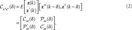
Second-order circularity is a property of probability density functions (pdf), whereby the distribution of a complex random variable z and its rotation e^𝒥φz are equal for any angle φ (Picinbono, 1994). Within the domain of second-order statistics, to account for complex random variables with non-circular pdf, we need to use both the covariance 𝒞_zz and pseudo-covariance 𝒫_zz matrices (Picinbono and Bondon, 1997)

For second-order circular (proper) random variables, the pseudo-covariance matrix vanishes, that is 𝒫_zz = 0, whereas for second-order non-circular (improper) random variables the pseudo-covariance matrix is non-zero, 𝒫_zz ≠ 0, and is generally complex-valued. The pseudo-covariance matrix 𝒫_zz can be written in terms of the covariances of its real and imaginary components

illustrating that for proper signals, the vanishing pseudo-covariance is due to equal powers in the real and imaginary channels, while the cross-covariance is skew-symmetric (Neeser and Massey, 1993).

For an uncorrelated random vector, both the covariance and pseudo-covariance matrices are diagonal (Eriksson and Koivunen, 2006). Examples of complex circular signals in signal processing research are QPSK and BPSK signals in communications, while most complex signals made complex by convenience of representation are non-circular. Examples include EEG signals, and complex-valued wind models (Mandic and Goh, 2009).

Consider a second-order stationary “augmented” complex random signal z^a(k) = [z^T(k), z^H(k)]^T and its augmented covariance matrix,

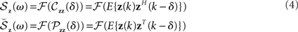
This matrix provides a complete description of the second-order statistics of z(k). The transformation of this matrix to the frequency domain gives the augmented spectral matrix (Picinbono and Bondon, 1997; Schreier and Scharf, 2003)

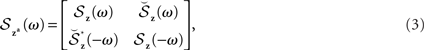
with the Fourier transforms of the covariance and pseudo-covariance matrices defined respectively as 𝒮_z(ω) and that is

where the symbol δ denotes a discrete time lag and ℱ(·) the Fourier transform operator.

While the power spectrum provides information on the distribution of signal power over a frequency range, the magnitude of the pseudo-spectrum characterizes the second-order circularity of the random variable in the frequency domain. The augmented spectral matrix in (3) is positive semidefinite which results in the condition (Picinbono and Bondon, 1997)

2.2 Complex Statistics: Kurtosis

Kurtosis has been used routinely to design contrast functions in BSS (Hyvärinen and Oja, 1997) and BSE algorithms (Cichocki et al., 1997). It is common to use the normalized kurtosis K_R(·) instead of the standard kurtosis kurt_R(·), as it allows for the comparison of the degree of non-Gaussianity of random variables, irrespective of the range of amplitudes. In (Ollila and Koivunen, 2009a), the relevance of this concept in the complex domain, together with as the relation between the kurtosis of the real and imaginary components of a complex random variable, kurt_R(z_r) and kurt_R(z_i) and the kurtosis of the complex random variable kurt_c(z) has been discussed.

The normalized kurtosis of a complex random variable (real-valued) can be defined as

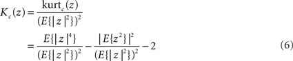
with

The first term in (6) is the normalized fourth order moment, the second term is the square of the circularity coefficient (Ollila, 2008), whereas kurt_c(z) in (7) is the real-valued kurtosis of the complex random variable z. Similar to the kurtosis of a real-valued Gaussian random variable, the value of K_c is zero for both circular and non-circular complex Gaussian random variables. Furthermore, for continuity, this measure makes kurtosis values of a sub-Gaussian complex random variable negative and that of a super-Gaussian complex random variable positive, irrespective of the degree of circularity/non-circularity (Douglas, 2007).

2.3 Complex-Valued Noise

The degree of non-circularity can be quantified by the circularity measure r, defined in (Ollila, 2008) as the magnitude of the circularity quotient where

measures the degree of non-circularity in the complex signal, with the pseudo-variance of the signal and the circularity angle θ = arg(ρ(z)) indicating orientation of the distribution. Note that for a purely circular signal, r = 0, with θ not providing additional information about the distribution.

This circularity measure can also be graphically interpreted using an ellipse (centered in the complex plane) of eccentricity ε and orientation α, such that r = ε² and θ = 2α (Ollila, 2008, Theorem 1). For ε = 0, the shape becomes a circle, which also indicates a circular signal with r = 0, while for the extreme case of ε = 1, corresponding to a highly non-circular signal with r = 1, the ellipse becomes elongated with a maximal major axis and minor axis of length zero. Note that the pseudo-variance of a general complex Gaussian distribution is then related to the elliptic shape by τ² = ε²e^ℱ2θ (Ollila and Koivunen, 2009b).

It is important to notice that the treatment of a noise vector v(k) in ℂ is different to that in the real domain (Picinbono and Bondon, 1997). While in ℝ only the variance of the noise signal is of concern, in ℂ it is necessary to also consider the pseudo-variance in order to completely model the noise. We therefore differentiate between the following cases of white noise.

1. Circular white noise, is considered white in terms of its diagonal covariance matrix, whereas the pseudo-covariance matrix vanishes, that is

where I denotes the identity matrix.

In the frequency domain, the covariance spectrum 𝒮_v(ω) (also power spectrum, or PSD) of the circular white noise is flat, while the pseudo-covariance spectrum (or pPSD) is zero.

2. Non-circular doubly white noise, is assumed white for both the real and imaginary components, however, the corresponding distributions and power levels may be different, such that

In this case, the power spectrum is flat across all frequencies, while the pseudo-spectrum is non-zero. As the noise becomes more non-circular (r → 1), the pseudo-spectrum approaches its upper-bound defined in (5), where for highly non-circular noise (r ~ 1), the magnitudes of the pPSD and PSD are similar. For a scalar complex white noise signal v(k), the relations between the correlation and pseudo-correlation and the respective spectra are given by

Examples of circular white Gaussian and Laplacian noise with unit variance are illustrated in the left hand column of Figure 1A, whereas the right hand column demonstrates two examples of non-circular white noise, with the top-right plot showing a non-circular Gaussian noise signal with circularity measure r = 0.81 with unit variance and pseudo-variance and the bottom-right plot illustrating the scatter plot of non-circular Laplacian noise with circularity measure r = 0.81 with unit variance and pseudo-variance of 0.45 − 𝒥0.66. Also note that in Figure 1A the value of the kurtosis is approximately zero for both the circular and non-circular Gaussian noise signals, whereas the kurtosis values for the circular and non-circular super-Gaussian noise signals follow the real-valued convention.

FIGURE 1

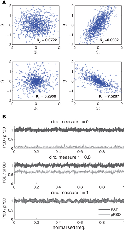
Figure 1. Illustration of white circular and doubly white complex-valued noises. (A) Scatter plots of complex white noise realisations. Top row: circular Gaussian noise (left) and non-circular Gaussian noise (r=0.81) (right). Bottom row: circular Laplacian noise (left) and non-circular Laplacian noise (r= 0.81) (right). The circularity measure r is defined in (8). The kurtosis values Kc are given for each case. (B) Power spectra (thick gray line) and pseudo-power spectra (thin gray line) of complex Gaussian noises with varying degrees of non-circularity r = {0, 0.8, 1}.

Figure 1B depicts the PSD and pPSD of circular (r = 0) white and non-circular doubly white Gaussian noise for the respective circularity measures r = {0.8,1}. Observe that the pseudo-spectrum is zero for the circular noise, while it has a magnitude of 0.64 for the noise with r = 0.8, and reaches it upper-bound of 1 in the third realization where the noise is highly non-circular (r = 1). For the Gaussian noise, the spectrum 𝒮(ω) = 1 and the pseudo-spectrum 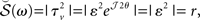across all frequencies, thus indicating that by increasing the eccentricity of the ellipse (degree of non-circularity), the magnitude of the pPSD approaches its maximum value of 1.

2.4 ℂℝ Calculus: Brief Overview

The ℂℝ calculus¹ (Kreutz-Delgado, 2006) allows for the analysis of functions that do not normally satisfy the stringent Cauchy–Riemann conditions of analyticity, such as real-valued cost functions of complex variables. Consider a typical cost function F(z): ℂ^N |→ ℝ, a real function of complex variables, which does not satisfy the Cauchy–Riemann properties, required for gradient calculations. However, using the ℂℝ calculus framework, it is possible to calculate the gradients of such functions directly in ℂ, and without the need to obtain derivatives of the real and imaginary components separately.

In the framework of ℂℝ calculus, F is taken as a function of the complex input vector z and its conjugate z^*, collectively termed the conjugate coordinates, that is

Note that although z and z* are not statistically independent, this does not affect the calculation of derivatives, defined as (Kreutz-Delgado, 2006)

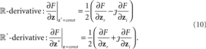
Also note that the direction of steepest descent is given by the derivative with respect to z^*, the ℝ^*-derivative. This can be shown by using the first order Taylor series expansion (TSE) of F (van den Bos, 1994); the magnitude of a small change in the function F is given by

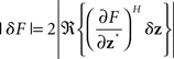
and the Cauchy–Schwarz Inequality shows that

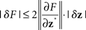
and so |δF| is maximized when across 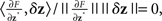or in other words the maximum change of the gradient is in the direction of the conjugate of the weight vector (Brandwood, 1983; Kreutz-Delgado, 2006). The operators 𝕽{·} and 𝕵{·}, where used, denote the real and imaginary part of a complex quantity, while 〈·,·〉 is the inner product operator.

Furthermore, in calculating derivatives of analytic functions, as defined, the ℝ^*-derivative vanishes and the derivative is equivalent to the Cauchy–Riemann derivative, demonstrating the flexibility of the framework. This can be illustrated through a simple example. Consider the non-analytic squared error cost function Then, ∂𝒢/∂z = z^* and ∂𝒢/∂z^* = z. In contrast, for the analytic function 𝓗(z) = z², ∂𝓗/∂z = 2z and ∂𝓗/∂z^* = 0. For further insight into ℂℝ calculus, we refer to the material in (Kreutz-Delgado, 2006; Mandic and Goh, 2009).

2.5 BSE of Complex Noisy Mixtures

The diagram in Figure 2 shows the complex BSE architecture, where at time instant k, the observed signal x(k) ∈ ℂ_N is given by a linear mixture

FIGURE 2

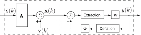
Figure 2. The noisy mixture model, and BSE architecture.

where is the vector of latent sources, A ∈ C^{N × N}, is the mixing matrix², and v(k) ∈ ℂ^N is the vector of additive doubly white Gaussian noise (non-circular). The model (11) has been widely used in EEG signal processing, for instance see (Cichocki and Amari, 2002; Sanei and Chambers, 2007). The sources are assumed to be with zero mean and distinct kurtosis values, while no assumptions are made about the circularity. The number of mixtures is assumed to be equal to that of the sources, however, in the case of noisy mixtures, an overdetermined mixture is necessary so as to estimate the second-order statistics of noise parameters.

The adaptive gradient descent algorithm at the extraction stage adapts the parameters of the demixing vector w such that the source signal with the largest (smallest) kurtosis,

is first extracted. The variance of y(k) can be written in an expanded form as

where the difference in 𝒞_ss(0) are absorbed into the mixing matrix A and the noise covariance matrix (due to the whiteness assumption).

In the same spirit, the normalized kurtosis of the extracted signal y(k) can be written as

thus having zero value for Gaussian noise. In a vectorized form, this is equivalent to

where

The next stage within the proposed BSE scheme is the deflation process which aims to remove the extracted source y(k) from the mixture x(k), such that

where the deflation weight coefficient vector is updated using an adaptive gradient descent algorithm detailed later in this section. In principle, for y(k) being an estimate of one of the original sources, say s_n(k), the ideal deflation weight vector should be equal to the nth column of the mixing matrix A, such that the effect of this particular source is removed from the mixture. Finally, a threshold can be set on the deflation process, so that extraction is continued until some or all the required sources have been successfully extracted (Thawonmas et al., 1998).

2.6 Cost Function

The cost function we employed for the extraction of general complex sources from noisy mixtures is given by

Note that 𝒥 ∈ ℝ, represents a modified version of the normalized kurtosis defined in (6) and is a generalization of the methodology presented in (Liu and Mandic, 2006). As illustrated in (13), the variance of y(k) contains the noise variance thus allowing us to remove the effect of noise from (17) such that only contributions from the latent sources are accounted for. Also note that while the noise variance is present in the cost function (17), its pseudo-covariance is not present, suggesting that the complex domain BSE based on kurtosis is unaffected by the pseudo-spectral effects of the additive noise; this is further elaborated in Section 3.

In the cost function (17), the parameter β dictates the order of extraction where for

1. β = 1, the order of extraction is from the high to low degree of non-Gaussianity (super-Gaussian sources are extracted first),

2. β = −1, the order of extraction is from low to high degree of non-Gaussianity (sub-Gaussian sources are extracted first).

The optimization of 𝒥 with respect to w can thus be stated as

where the norm of the demixing vector is constrained to unity to avoid very small coefficient values.

Rewriting and simplifying (17) in terms of (13) and (16) results in

where

Notice that and is equal to unity only if one of the components in the vector u is non-zero. Given the constraint on |ú|, the solution to the optimization of (19) is a vector ú_opt of unit norm such that u_opt has a single non-zero component at a position corresponding to the diagonal element in K_c(s) having the largest magnitude. For this to be valid, a demixing vector assumes the form w_opt = A^H#u_opt, where the symbol (·)# denotes the matrix pseudo-inverse operator (Liu and Mandic, 2006).

2.7 Adaptive Algorithm for Extraction

Optimization of (17) is performed using an adaptive gradient descent algorithm which updates the values of w so as to maximize the modified normalized kurtosis and thus minimize the cost function 𝒥(w). Based on Section 2.4, the gradient³ is thus expressed as

where φ(y(k)) is used for simplification and m_ℓ(y) and p_ℓ(y) are respectively the ℓ-th moment and pseudo-moment at time instant k (the time index dropped), estimated using the moving average estimators

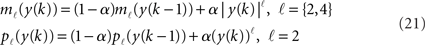
where α ∈ [0,1] is the forgetting factor.

The kurtosis-based BSE update algorithm (K-cBSE) for the demixing vector is thus given by

and its expanded version is given in (22),

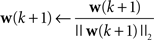
where μ is the small positive step-size. To preserve the unit norm property, the demixing vector is normalized at each iteration, that is

Notice that in extracting circular sources, the moment p_ℓ vanishes, further simplifying the algorithm. Moreover, as mentioned earlier, the cost function and thus the gradient descent algorithm are not dependent on the pseudo-variance of the noise, The estimation of the noise variance can be performed using a subspace method, as described in (Hayes, 1996). It is thus essential that the number of observations is larger than the number of sources, N > N_s, so as to allow for the estimation of the noise variance via eigenvalues of the observation covariance matrix 𝒞_xx, that is

The subspace method can be briefly summarized as follows. We can assume Rank(ϒ) = N_s if A is of full rank and 𝒞_ss is non-singular. Then, the (N − N_s) eigenvalues of ϒ are zero and hence the (N − N_s) eigenvalues of 𝒞_xx are equal to

2.8 Modifications to the Update Algorithm

In order to enhance the performance of the online gradient descent algorithm, adaptive step-size update algorithms are considered. We consider the complex-valued Farhang–Ang type variable step-size (VSS) algorithm (Ang and Farhang-Boroujeny, 2001) and the complex-valued generalized normalized gradient descent (GNGD) type algorithm (Mandic, 2004).

At each iteration k, the VSS algorithm minimizes the cost function 𝒥 in (17) with respect to μ(k − 1) to provide the update of the step-size, given as

where and η and γ are step-sizes.

The GNGD-type algorithm is based on a normalized version of (22), given by

where ε(k) is an adaptive regularization parameter. The gradient adaptive regularization parameter is then given by

where ρ is a step-size. The derivation of the algorithm is given in the Appendix.

2.9 Adaptive Algorithm for Deflation

The deflation procedure insures that after each extraction stage, the estimated source is removed from all the mixture vectors, so that the next source with maximum (minimum) kurtosis can be extracted. This can be achieved based on the cost function (Thawonmas et al., 1998)

which is minimized with respect to the deflation weight coefficient We use x_n(k) to denote the mixture at the nth extraction stage, which is given by vectors

Given an invertible mixing matrix A, the vector is ideally equal to a column of A⁻¹, which corresponds to the nth extracted source y_n(k). The gradient can thus be calculated as

and the online algorithm for BSE then becomes

with μ_d a step-size. The drawback of this method is that any errors in the deflation process will propagate and affect the extraction and deflation of subsequent stages. It is therefore important that the step-size parameter is set appropriately for each nth deflation stage to ensure successful removal of the extracted source y_n(k).

In the design of complex adaptive algorithms, it is common to utilize a widely linear model to ensure that the algorithm is capable of processing the generality of complex signals (Mandic and Goh, 2009). In the case of the update for the deflation weight coefficient (30), however, a linear model is considered as the original BSS mixing model (11) is strictly linear and thus a widely linear deflation model is not required. For more detail on BSE based on widely linear predictability, see (Javidi et al., 2010).

3 Results and Discussions

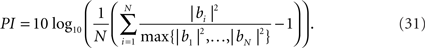
We shall consider extraction of both synthetic and real-world sources from noise-free and noisy mixtures, with various degrees of complex non-circular noise levels. The performance for the synthetic data were measured using the performance index (PI; Cichocki and Amari, 2002) given by

where u = A^Hw = [u₁,…,u_M].

For each synthetic experiment, the results were produced through averaging 100 independent trials. The mixing matrix A was generated randomly as a full rank complex matrix. The values of the extraction and deflation step-size μ were set empirically, and the forgetting factor α in (21) was set as 0.975. The complex additive Gaussian noise was both of circular white with circularity measure r = 0 and non-circular doubly white with r = 0.93. The real-world sources were the electroencephalogram data corrupted by power line noise and electrooculogram (EOG) artifacts.

3.1 Benchmark Simulation 1: Synthetic Sources

In the first set of simulations, a noise-free mixture of three complex sources with various degrees of circularity and N = 5000 samples were generated and mixed using a 3 × 3 mixing matrix. These signals are illustrated in Figure 3 and their properties listed in Table 1. Extraction was performed in order from highest to lowest kurtosis, hence the value of β = 1 in (17).

FIGURE 3

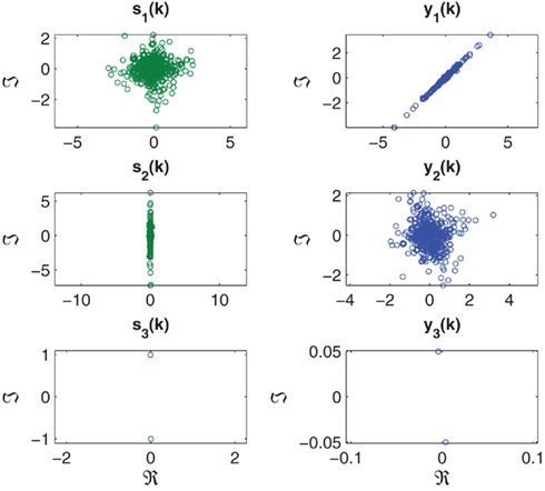
Figure 3. Scatter plot of the complex-valued sources s₁(k), s₂(k), and s₃(k), with the signal properties described in Table 1 (left hand column). Scatter plot of estimated sources y₁(k), y₂(k), and y₃(k), extracted according to a decreasing order of kurtosis (β = 1) (right hand column).

TABLE 1

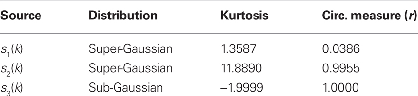
Table 1. Source properties for noise-free extraction benchmark simulation 1.

In the first experiment, the performance of the algorithm (22) using the adaptive step-size methods was compared in the extraction of the first source with the value of μ set to 0.01. It can be seen from the performance curves in Figure 4 that the best performance was achieved using the GNGD method with a PI of around −45 dB at the steady-state. The performance curve resulting from the normalized method indicates successful extraction with a PI of around −25 dB. The performance of the algorithm using the standard step-size and VSS were comparable, with a PI of around −20 dB. In the following simulations, the GNGD based K-cBSE algorithm is utilized.

FIGURE 4

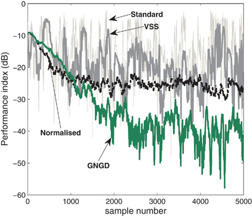
Figure 4. Comparison of the effect of step-size adaptation on the performance of algorithm (22) for the extraction of a single source.

In the next set of simulations, we considered the extraction of all the three sources (Figure 3). The value of μ was set respectively to 0.01, 0.008, and 10⁻⁵ for the consecutive extraction stages. As shown in Figure 5, the algorithm successfully extracted all the three sources, as indicated by a PI of less than −20 dB at the steady-state for the extraction iteration i = {1,2,3}, converging to steady-state after 2500 samples in the first extraction stage (i = 1) and around 1000 samples in the second and third extraction stage (i = {2,3}). The decreasing PI value at each consecutive extraction stage can be attributed to the unavoidable errors accumulated in the deflation. The scatter plot of the three estimated sources y₁(k), y₂(k), and y₃(k) are illustrated in Figure 3. The normalized kurtosis of the estimated sources were respectively calculated as K_c(y₁) = 11.8425, K_c(y₂) = 1.3599, and K_c(y₃) = −1.9956 corresponding to those of the original sources, given in Table 1; the scale and rotation ambiguities of the source estimates are also visible.

FIGURE 5

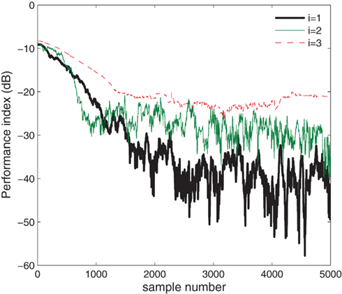
Figure 5. Extraction of complex circular and non-circular sources from a noise-free mixture based on kurtosis.

3.2 Benchmark Simulation 2: Noisy Mixture

In the next experiment, we considered the extraction of a complex-valued source from a noisy mixture. Three sources of N = 5000 samples were considered (see Table 2; Figure 6) and mixed using a randomly generated 4 × 3 mixing matrix A. The additive noise was doubly white Gaussian noise with variance and pseudo-variance 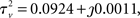estimated using the subspace method described in Section 2.5. The sources were extracted in an increasing order of kurtosis (β = −1) with the step-size μ = 0.5. The scatter plot of the first estimated source with the smallest kurtosis, y₁(k) is illustrated in Figure 6 with a calculated normalized kurtosis of K_c(y₁) = −1.8002, which is within a 10% range of the true value, given in Table 2. The PI, shown in Figure 7, demonstrates a fast convergence to a value of around −40 dB in approximately 1000 samples, and continuing a steady convergence to −50 dB by 5000 samples.

TABLE 2

Table 2. Source properties for noisy extraction in benchmark simulation 2.

FIGURE 6

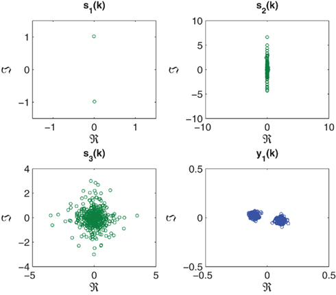
Figure 6. Scatter plots of the original sources s₁(k), s₂(k), and s₃(k). The first estimated source y₁(k) is shown in the bottom-right plot.

FIGURE 7

Figure 7. Extraction of a complex-valued source from a noisy mixture, with the source properties given in Table 2.

It was shown in Section 2.5 that the performance of the algorithm (22) is not affected by the degree of circularity of the additive noise, such that doubly white noise is treated in a similar manner to circular white noise, where the pseudo-covariance vanishes. This was explored experimentally by systematically analyzing the effect of various noise levels on the BSE algorithm (22). The circularity measure r was varied from a value of r = 0 (circular) to a value of r = 0.9998 (highly non-circular), while the signal-to-noise ratio (SNR) was adjusted from a near-zero noise SNR of 50 dB to a high noise environment with SNR value of −10 dB. The initial values were generated randomly and PI was averaged over 100 trials. Figure 8 illustrates the performance curve for the different variations in the noise properties, and confirms that while the performance is dependent on the SNR value, it does not vary with changes in the degree of noise non-circularity. In addition, the maximum effective range of the algorithm in extracting sources (PI < −20 dB) can be estimated as an SNR of 1 dB.

FIGURE 8

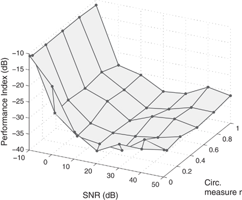
Figure 8. Comparison of the performance of algorithm (22) with respect to changes in the SNR and the degree of noise circularity.

3.3 EEG Artifact Extraction

In order to obtain useful information from EEG data in real-time, it is often necessary to perform post-processing to remove artifacts such as line noise and biological artifacts including those pertaining to eye movement, captured in the form of EOG and facial muscle activity represented as electromyogram (EMG). Removal of the effect of such signals from the contaminated EEG has been subject of study in previous years, with several methodologies introduced that attempt to accomplish this utilizing both online and offline algorithms (Vigário, 1997; Jung et al., 2000; Delorme et al., 2001, 2007; Barbati et al., 2004; Greco et al., 2005; Kumar et al., 2009). While offline algorithms are suitable for processing the recorded EEG data in clinical applications, it is necessary to utilize online algorithms for real-time applications such as those encountered in brain computer interface (BCI) scenarios.

In (Kumar et al., 2009) the authors propose an online algorithm whereby the recorded EEG signals are transformed to the wavelet domain and the EOG contaminants are removed using an adaptive recursive least squares (RLS) algorithm, before transforming the signal back to the time domain. Simulations demonstrate good performance from the algorithm, however, it would be advantageous to perform all the necessary processing in the time domain, as this way the signals are retained in their original form and less computation is required.

In its basic form, ICA can be applied to the contaminated EEG recording and the artifacts removed through visual inspection. As detailed in (Vigário, 1997), an ICA algorithm separates the recorded EEG mixture into its original sources as independent components (ICs), with artifact sources identified and removed. In semi-automatic (Greco et al., 2005) and automatic (Delorme et al., 2001) artifact removal methodologies, several classifications (markers) based on the statistical characteristics of the ICs are considered that allow for the detection of artifacts in the contaminated EEG, which are then compared against thresholds that determine the rejection of particular components. In these methods, both the kurtosis and entropy of ICs have been utilized to identify and remove the artifacts. While the EEG mixtures typically have near-zero kurtosis values, artifacts such as EOG exhibit peaky distributions with highly positive kurtosis values (Delorme et al., 2001), while periodic power line noise has a highly negative kurtosis value. This has been used as the main discrimination in defining classifications based on the fourth order moment.

3.3.1 Data acquisition and method

Our aim is to remove artifacts as independent sources extracted from the recorded EEG mixture directly in the time domain. To this end, the contaminated EEG signals were paired as the real and imaginary components of a complex signal and processed using the architecture described in Section 2.5. In this manner, the phase–amplitude relationship and the full cross-statistical information between symmetric electrode pairs are contained in the corresponding complex-valued EEG signal, and allow for the simultaneous processing of both channels. Further iterations of the extraction process can then be used to obtain the individual pure EEG signals, or even, pipelined to a further post-processing stage, which would then extract the EEG signals based on a desired fundamental property, such as predictability.

The electrodes were placed according to the 10–20 system (Figure 9), and sampled at 256 Hz for 30 s. The EEG activity was recorded from electrodes placed at positions Fp1, Fp2, C3, C4, O1, O2 with the ground placed at Cz, while the EOG activity was recorded from the vEOG and hEOG channels with electrodes placed above and on the side of the left eye socket.

FIGURE 9

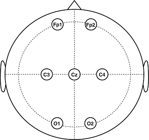
Figure 9. Placement of the EEG electrodes on the scalp according to the recording 10–20 system.

Three studies were performed with the aim to remove the artifacts simultaneously. While the rejection of the power line noise artifact is feasible by passing the recorded EEG signals through a notch filter, this solution also leads to the removal of useful information around the 50-Hz range pertaining to the EEG signals, in particular those within the gamma band (25–100 Hz). It would therefore be desirable to automatically extract the line noise artifact along with the biological artifact from the corrupted EEG signals. In the first study we consider the removal of EOG artifacts (“Eyeblink” set), the second study focused on eye muscle artifacts from rolling the eyes (“Eyeroll” set), whereas the third study addressed the removal of muscle activity from raising the eyebrow (“Eyebrow” set).

In all the studies, the temporal signals from each channel pair were combined to form three complex EEG channels, given by

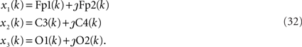
This construction of the complex EEG signals allows for the simultaneous processing of the amplitude and phase information using the K-cBSE algorithm (22). Note that the EOG channels were not part of the mixtures considered. They are only used to assess the performance of the proposed BSE algorithm in the extraction of the EOG artifacts.

3.3.2 Performance measures

As we have no knowledge of the mixing process, the PI (31) is not applicable for this case and thus several alternative quantitative and qualitative measures were used for the evaluation of the algorithm performance. These are briefly discussed below.

1. Quantitative metrics

(a) Kurtosis: The kurtosis values K_c of the complex extracted signals indicate the success of the algorithm in extracting super-Gaussian or sub-Gaussian artifact in a specified order. In addition, the magnitude of the kurtosis K_R of the real and imaginary components of the extracted sources are used to automatically select desired components.

(b) Power spectra Correlation: In a similar manner to (Barbati et al., 2004), the correlation coefficient between the power spectra of the complex-valued recorded artifact (e.g., EOG) and extracted sources, and likewise, the correlation coefficient between the pseudo-power spectra of the complex-valued recorded artifact and the extracted sources is calculated. This measure indicates the degree of similarity between the extracted and originally recorded artifact, and can be used to automatically select the extracted source pertaining to the biological artifact, while also quantifying the degree of performance of the extraction algorithm.

2. Qualitative metrics

(a) Hilbert–Huang Time–Frequency Analysis: By employing time–frequency (T–F) analysis using the Hilbert–Huang (H–H) transform (Huang et al., 1998; Huang and Shen, 2005), we can qualitatively assess the extraction performance through comparison of the frequency components of the mixture and extracted source during the recording session. Also, the T–F analysis of the extracted artifacts will demonstrate the corresponding frequency components and their changes over time, making it possible to assess the quality of the extraction procedure over the recording time. In comparison to Fourier transform based T–F analysis, such as the Short-Time Fourier Transform, the H–H transform results in much more detailed spectrogram for a given resolution. The intrinsic mode functions (IMFs) required by the H–H transform were obtained using a multivariate empirical mode decomposition (MEMD) algorithm (Rehman and Mandic, 2010), where the real and imaginary component of the complex-valued signals were taken as a single multivariate signal and processed simultaneously. It was observed that this resulted in a spectrogram with better resolution than those obtained through the separate processing of the individual components using the standard EMD algorithm.

(b) Power Spectral Distribution: The power and pseudo-power spectra of the complex-valued extracted artifacts were compared to those belonging to the complex-valued recorded artifact. In addition, the pseudo-spectrum demonstrates the quality of the proposed method in extracting non-circular sources. It is also possible to consider the cross-spectrum of the recorded and extracted sources (Palmer et al., 2009).

3.3.3 Case Study 1 – EOG extraction

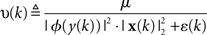
The “Eyeblink” dataset contained the EEG recordings contaminated with eye blink artifact as well as line noise. The recorded EEG and EOG signals are plotted in Figure 10A, where the effect of the EOG activity is pronounced in the frontal lobe (Fp1 and Fp2 channels), with the effect diminishing with an increase in the distance of the electrodes to the eyes. The effect of the line noise is also visible on the occipital O1 and O2 channels. The H–H T–F spectrogram (Figure 10B) describes the frequency changes of the ensemble average of the six EEG channels over the recording period. In correspondence with the time plot, the EOG artifacts are visible (with a duration of around 1 s); constant frequency components are seen around the 50-Hz range due to the line noise. Note that due to the low sampling rate of the recording device, the 50-Hz frequency component is not well defined in the T–F analysis and results in scattering of frequency components between 40 and 60 Hz.

FIGURE 10

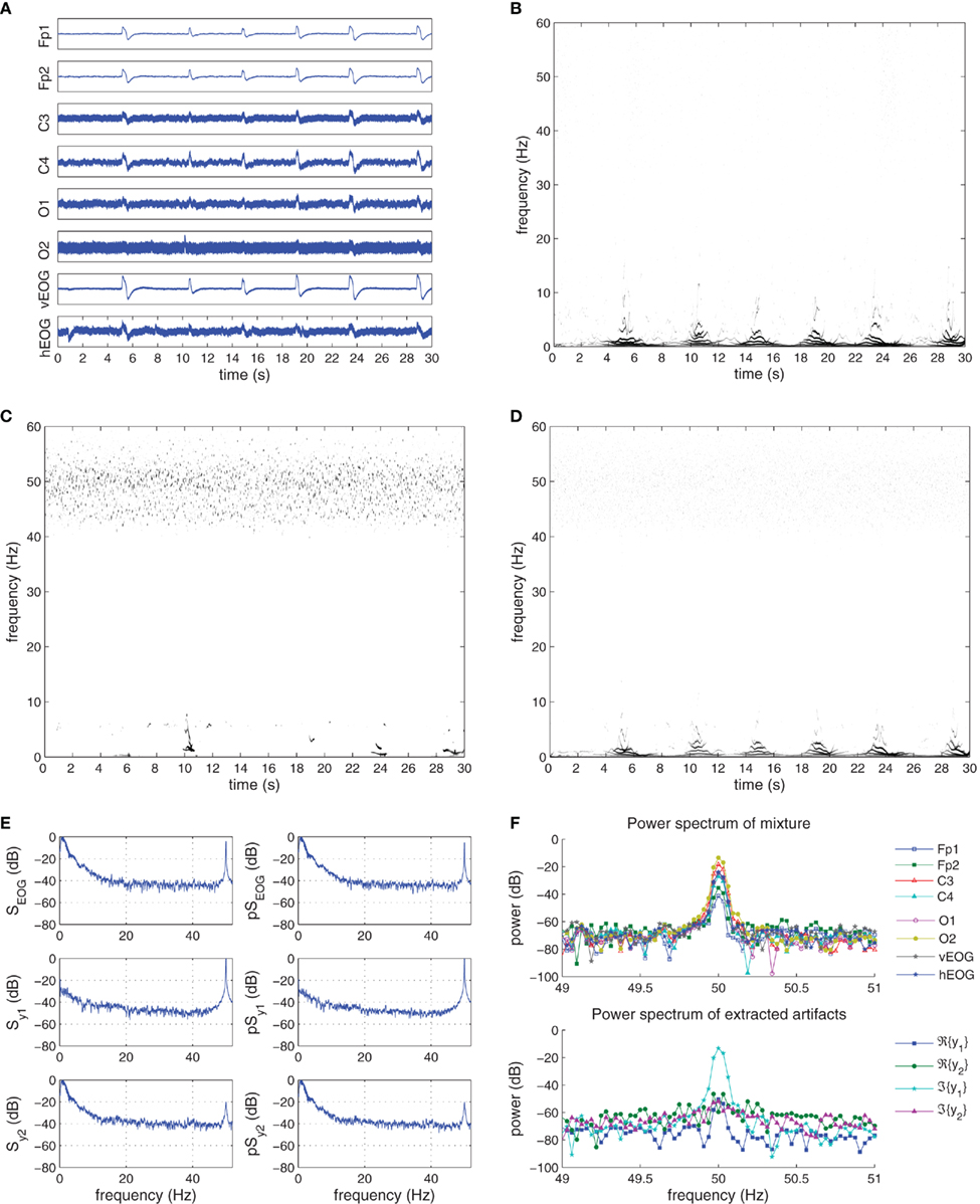
Figure 10. Recorded and extracted artifacts from the “EYEBLINK” set. (A) Recorded EEG signals from the “EYEBLINK” set. (B) The Hilbert–Huang time–frequency plot of the recorded EEG signals. (C) The Hilbert–Huang time–frequency plot of the extracted line noise 𝕵{y₁(k)}. (D) The Hilbert–Huang time–frequency plot of the extracted EOG 𝕽{y₂(k)}, 𝕵{y₂(k)}. (E) The power spectra (S) and pseudo-spectra (pS) of the recorded EOG, and the extracted signals y₁(k) and y₂(k). (F) The power spectra (S) and pseudo-spectra (pS) of the recorded EOG, and the extracted signals y₁(k) and y₂(k). (G) Frequency components of the recorded EEG signals and the extracted artifacts at the 50-Hz frequency range. After extraction, the power line noise is contained in 𝕵{y₁}.

The complex EEG signals formed using (32) were processed using the K-cBSE algorithm with the value of μ = {5,0.09} and β = {−1,1} for the consecutive iterations and α = 0.975. The choice of value for β ensures that the line noise is initially extracted, followed by the EOG components in the second iteration. The normalized kurtosis values of the original real-valued EEG signals and the extracted EEG signals are given in Tables 3 and 4.

TABLE 3

Table 3. Normalized kurtosis values of the recorded EEG/EOG signals in real- and complex-valued form.

TABLE 4

Table 4. Normalized kurtosis values of the extracted artifacts, and the correlation coefficient of the power and pseudo-power spectra respectively with the spectra of the recorded EOG.

The order of the extracted complex signals were as expected, with the first extracted source y₁(k) (line noise) being sub-Gaussian and y₂(k) (EOG) super-Gaussian. The imaginary component of y₁(k) had the smallest kurtosis, and was automatically chosen as the extracted line noise source, while the near-zero kurtosis of the real component 𝕽{y₁(k)} indicates an EEG source. Also, both components of the second extracted source, having a high kurtosis value, were considered as the extracted EOG sources. Figure 10C shows the T–F plots of the imaginary components of the first extracted signal y₁(k) where the presence of the power line artifact is seen, while in Figure 10D the T–F plot of the real and imaginary components of y₂(k) is shown where the frequency components of the EOG artifacts are seen.

We next concentrate on the power spectrum and pseudo-power spectrum of the complex EOG signal, constructed in a similar manner to that in (32); the extracted sources y₁(k) and y₂(k) are depicted in Figure 10E. Notice that the distribution of power 𝒮_EOG and pseudo-power is concentrated respectively in the frequency range (0–5) Hz and 50 Hz. The spectrum and pseudo-spectrum of the first extracted source can be seen to contain around 0 dB of power for a frequency of 50 Hz, while having an average power of −40 dB in the (0–5) Hz frequency range. These results can also be seen by comparing the frequency components of the recorded EEG mixture and extracted artifactual sources around the 50-Hz range, shown in Figure 10G. While the presence of the power line artifact is evident in all recorded channels, after the extraction procedure the 50-Hz frequency component is only present in 𝕵{y₁(k)}. Likewise, the spectra of y₂(k) illustrate the diminished effect of the line noise source with a power of −20 dB, while retaining the frequency components of the EOG in the low frequency range. To quantify the observed results, the correlation coefficient between the recorded EOG’s PSD and pPSD and those of the extracted sources were calculated (Barbati et al., 2004) and presented in Table 4. For the extracted source y₁(k) these values were respectively 0.2313 and 0.2847, whereas for the source y₂(k) they were 0.9698 and 0.9822. The correspondence of the results between the power and pseudo-power spectra demonstrates the effectiveness of the methodology in extracting artifacts in the complex domain.

3.3.4 Case Study 2 – Eye muscle artifact extraction

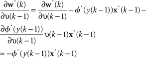
The “Eyeroll” dataset had contained artifacts from round movement of the eye during the recording session with EOG activity from eye blinks, shown in Figure 11A and kurtosis values given in Table 3.

FIGURE 11

Figure 11. Recorded and extracted artifacts from the “EYEROLL” set. (A) Recorded EEG signals from the “EYEROLL” set. (B) The Hilbert–Huang time–frequency plot of the recorded EEG signals. (C) The Hilbert–Huang time–frequency plot of the extracted line noise 𝕽{y₁(k)}. (D) The Hilbert–Huang time–frequency plot of the extracted EOG 𝕽{y₂(k)}, 𝕵{y₂(k)}. (E) The power spectra (S) and pseudo-spectra(pS) of the recorded EOG, and the extracted signals y₁(k) and y₂(k). (F) Frequency components of the recorded EEG signals and the extracted artifacts around the 50-Hz frequency range. After extraction, the power line noise is contained in 𝕽{y₁}.

The resultant electrical activity from the artifacts were recorded using the vEOG and hEOG channels, with EOG activity seen on the vEOG channel at time instants 5, 13, 17, 23, 25, and 29 s, and eye muscle activity present more clearly on the hEOG channel with a duration of around 2 s. The eye muscle artifact was present on all six EEG channels, while the EOG artifact is strong on the Frontal lobe electrodes and the effect of the power line noise is seen more strongly on the central and occipital lobe electrodes. The H–H T–F analysis of Figure 11B illustrates the presence of frequency components up to 10 Hz, as well as scattered frequencies belonging to the 50-Hz power line noise.

In the extraction procedure, the step-size of the K-cBSE algorithm was μ = {5,0.2} and β = {−1,1}, while α = 0.975. The T–F analysis of the extraction are illustrated in Figures 11C,D, and the kurtosis values of the complex-valued extracted signals and their real and imaginary components given in Table 4.

The real component of the first extracted source, 𝕽{y₁(k)}, having the smallest kurtosis of K_c(𝕽{y₁}) = −1.1958 contained the power line noise artifact. The eye muscle activity and EOG artifacts were collectively extracted using the real and imaginary components of the second extracted source y₂(k). The five instances of the eye muscle activity and the EOG can be detected in Figure 11D, while the lack of power line noise frequency components in the 50-Hz range is visible.

These results were also confirmed based on the power spectra of the recorded artifacts and the extracted sources, given in Figure 11E. While the PSD and pPSD of the complex-valued y₁(k) contained the 50-Hz components, these were suppressed to −40 dB in the spectra of y₂(k). The frequency components of the mixture channels and extracted artifacts in the 50-Hz range also showed that the line noise artifact was successfully removed (see Figure 11F). Conversely, the spectral components pertaining to the eye muscle and EOG artifacts are present in the PSD and pPSD of y₂(k) corresponding to the (0–10) Hz range of the PSD and pPSD of the complex-valued EOG. The correlation coefficient between the PSD spectra of the complex-valued recorded EOG channel and extracted source y₂(k) is 0.8244, while the correlation between the pPSD spectra was 0.8222; these values were respectively 0.0792 and 0.1844 for y₁(k).

3.3.5 Case Study 3 – EMG extraction

In the “Eyebrow” set, the EEG mixture was heavily contaminated with EMG artifacts from raising the eyebrows, and are shown in Figure 12A with kurtosis values given in Table 3. The EMG signals were recorded using the vEOG and hEOG electrodes, with the effect more prominent on the vEOG recording. All EEG channels were affected by the artifact, though this is not clearly visible in the occipital lobe channels due to the strong presence of power line noise. In the T–F domain (Figure 12B) the EMG frequency range had a large span containing both low and high frequency components, present in the duration of the raising of the eyebrows and lasting for around 2 s. In addition, the 50-Hz frequency component cloud reflecting the power line noise can also be seen.

FIGURE 12

Figure 12. Recorded and extracted artifacts from the “EYEBROW” set. (A) Recorded EEG signals from the “EYEBROW” set. (B) The Hilbert–Huang time–frequency plot of the recorded EEG signals. (C) The Hilbert–Huang time–frequency plot of the extracted line noise 𝕽{y₁(k)}. (D) The Hilbert–Huang time–frequency plot of the extracted EMG 𝕽{y₂(k)}, 𝕵{y₂(k)}. (E) The power spectra (S) and pseudo-spectra (pS) of the recorded EMG, and the extracted signals y₁(k) and y₂(k). (F) Frequency components of the recorded EEG signals and the extracted artifacts around the 50-Hz frequency range. After extraction, the power line noise is contained in 𝕵{y₁}.

The extraction of the artifacts was performed using the K-cBSE algorithm (22) with step-size μ = {2,0.2}, β = {−1,1} and α = 0.975.

As shown in Figures 12C,D, the algorithm successfully extracted the power line noise as the imaginary component of the first extracted signal y₁(k) and the EMG signal as the real and imaginary components of the second extracted signal y₂(k). From the T–F plot of y₂(k) in Figure 12D, the complete EMG frequency component range was successfully extracted, with power line noise frequency components not present.

Considering the power spectra 𝒮_EMG and pseudo-power spectra in Figure 12E, the spectral distribution of the power and pseudo-power spectral density were strong in the (0–10) Hz range with an amplitude of around −10 dB and in the (20–40) Hz range, though having a much lower value. In addition, a single spike at 50 Hz of amplitude −10 dB indicates the presence of power line noise. After the extraction, the power line noise was contained in the spectra of the y₁(k) while the (0–10) Hz and (20–40) Hz frequency components were present in the PSD and pPSD of y₂(k). For the “Eyebrow” set, the spectra correlation coefficients between 𝒮_EMG and and those of y₁(k) and y₂(k) were respectively {0.1287,0.1078} and {0.7593,0.7906}. Also, the 50-Hz frequency range for the contaminated mixture and the extracted artifacts are shown in Figure 12F. It can be seen that after the extraction procedure, the 50-Hz component is contained in 𝕵{y₁(k)}, while in comparison to the EOG and eye muscle extracted components from the “Eyeblink” and “Eyeroll” studies (see Figures 10G and 11F), components 𝕽{y₂(k)} and 𝕵{y₂(k)} had a higher power level in this range, reflecting the wider frequency range of the EMG artifact.

3.3.6 EEGs after EOG and 50 Hz power line artifacts removal.

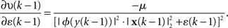
Figure 13 shows the EEG waveforms after the extraction of “Eyeblink,” “EyeRoll,” “EyeBrow,” and 50 Hz noise artifacts. The top two plots compare the proposed method with the widely linear prediction based one in (Javidi et al., 2010). Notice for the first two EEG electrodes Fp1 and Fp2, the predictor-based technique in (Javidi et al., 2010) performed well, with the successful removal of the Eyeblink artifact. However, it performed poorly in terms of the 50-Hz noise removal, which caused the “Eyeblink” artifact to be present (but attenuated) in the remaining EEG electrodes. Comparing Figure 13C with Figure 11A, it is clear that the “EyeRoll” artifact was either heavily attenuated or removed; whereas comparing Figure 13D with Figure 12A demonstrates that it is quite challenging to remove completely the “EyeBrow” artifact; however, the 50-Hz noise has been removed almost perfectly, as illustrated by comparing the bottom plots of Figures 12A and 13D.

FIGURE 13

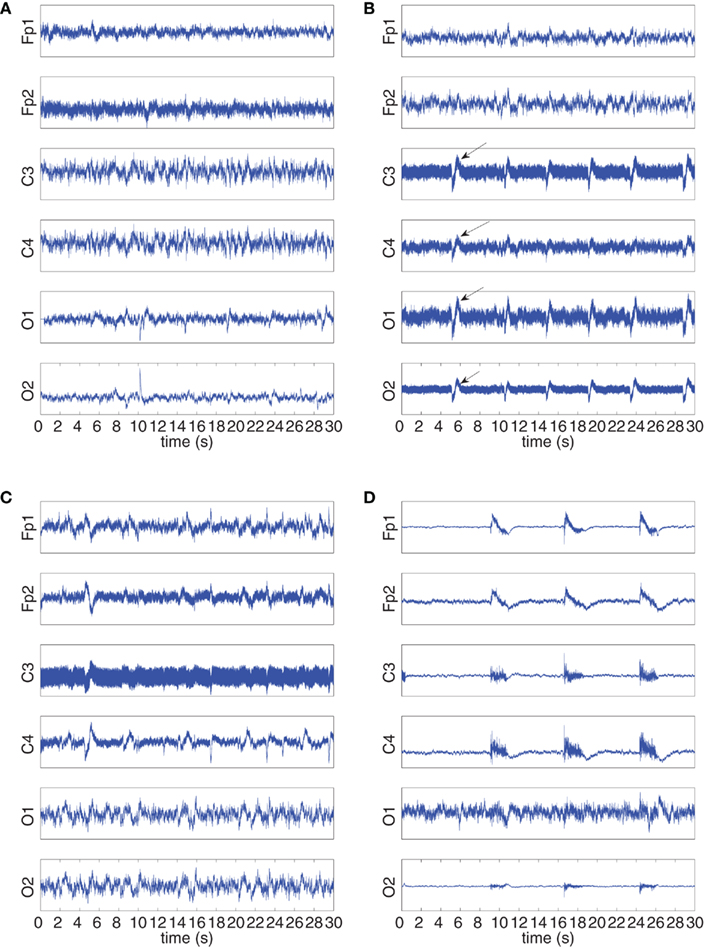
Figure 13. EEG after extracting artifacts from the “EYEBLINK,” “EYEROLL,” and “EYEBROW” set. (A) yYEBLINK: Kurtosis-based method. (B) EYEBLINK: Predictor-based method in (Javidi et al., 2010). (C) EYEROLL: Kurtosis-based method. (D) EYEBROW: Kurtosis-based method.

4 Discussion

Both qualitative and quantitative metrics have showed that the kurtosis-based extraction method yields enhanced results for real-time extraction of artifacts. Excellent results were obtained for the removal of eye blink, eye roll, and power line artifacts. Although artifacts arising from eye rolling and raising the eye brow might seem similar to that of an eye blink, it is much more challenging to perform their complete removal in the context of real-time EEG processing, as they involve longer firing of larger groups of muscles. These are critical cases, as the EMG source goes into saturation; and to our knowledge, these artifacts have not been considered before in the literature. These results are promising, as our technique operates real-time, in contrast to methods such as in (Vigário, 1997; Jung et al., 2000; Delorme et al., 2001, 2007; Barbati et al., 2004; Greco et al., 2005; Kumar et al., 2009). The advantage of the proposed kurtosis-based method as compared to our previous method (Javidi et al., 2010) is also in that the proposed method allows us to select a particular artifact to be extracted. For instance, if we wish only the EOG artifact such as eye blink to be removed, the parameter β in (22) can be set to unity; whereas in (Javidi et al., 2010), we do not have full control over which artifact is going to be extracted.

5 Conclusion

Blind source extraction of the generality of complex-valued signals based on the degree of non-Gaussianity and from noisy mixtures has been addressed. A cost function based on the normalized kurtosis has been utilized to perform blind extraction, and the corresponding online algorithm¹ (K-cBSE) has been derived. The existence and uniqueness of the solutions have been discussed and VSS variants of to the algorithm have been addressed. It has been shown that the algorithm is robust to the degree of non-circularity of the additive noise and the success of the algorithm over increasing noise levels has been demonstrated. Simulations in noise-free and noisy environments illustrate the successful performance of the algorithm in the extraction of both circular and non-circular signals, while the extraction of EOG and EMG artifacts from recorded EEG signals in real-time demonstrate a practical application for the proposed methodology.

Conflict of Interest Statement

The authors declare that the research was conducted in the absence of any commercial or financial relationships that could be construed as a potential conflict of interest.

Footnotes

1. ^Also known as Wirtinger calculus.
2. ^If a mixing process is considered for the noise given by B, the vector w^H in the subsequent equations can be replaced by υ^H = w^HB. This does not affect our algorithm, for the normalized kurtosis of Gaussian noise is unconditionally zero.
3. ^Since the normalized kurtosis 𝒥is real-valued, the conjugate gradient corresponds to the maximum change of the gradient.
4. ^This work was supported by the EPSRC grant EP/H026266.

References

Amari, S., Douglas, S. C., Cichocki, A., and Yang, H. H. (1997). “Novel on-line adaptive learning algorithms for blind deconvolution using the natural gradient approach,” In Proceedings of the 11th IFAC Symposium on System Identification, Kitakyushu, Vol. 3, 1057–1062.

Anemüller, J., Sejnowski, T. J., and Makeig, S. (2003). Complex independent component analysis of frequency-domain electroencephalographic data. Neural Netw. 16, 1311–1323.

Pubmed Abstract | Pubmed Full Text | CrossRef Full Text

Ang, W.-P., and Farhang-Boroujeny, B. (2001). A new class of gradient adaptive step-size LMS algorithms. IEEE Trans. Signal Process. 49, 805–810.

CrossRef Full Text

Barbati, G., Porcaro, C., Zappasodi, F., Rossini, P. M., and Tecchio, F. (2004). Optimization of an independent component analysis approach for artifact identification and removal in magnetoencephalographic signals. Clin. Neurophysiol. 115, 1220–1232.

Pubmed Abstract | Pubmed Full Text | CrossRef Full Text

Barros, A. K., and Cichocki, A. (2001). Extraction of specific signals with temporal structure. Neural Comput. 13, 1995–2003.

Pubmed Abstract | Pubmed Full Text | CrossRef Full Text

Bell, A. J., and Sejnowski, T. J. (1995). An information-maximisation approach to blind separation and blind deconvolution. Neural Comput. 7, 1129–1159.

Pubmed Abstract | Pubmed Full Text | CrossRef Full Text

Bingham, E., and Hyvärinen, A. (2000). A fast fixed point algorithm for independent component analysis of complex valued signals. J. Neural Syst. 10, 1–8.

CrossRef Full Text

Brandwood, D. H. (1983). A complex gradient operator and its application in adaptive array theory. IEE Proc. F Commun. Radar Signal Process. 130, 11–16.

CrossRef Full Text

Cichocki, A., and Amari, S. (2002). Adaptive Blind Signal and Image Processing, Learning Algorithms and Applications. Chichester: Wiley.

Cichocki, A., Thawonmas, R., and Amari, S. (1997). Sequential blind signal extraction in order specified by stochastic properties. Electron. Lett. 33, 64–65.

CrossRef Full Text

Delorme, A., Makeig, S., and Sejnowski, T. (2001). “Automatic artifact rejection for EEG data using high-order statistics and independent component analysis,” in International Workshop on ICA, San Diego, USA, 457–462.

Delorme, A., Sejnowski, T., and Makeig, S. (2007). Enhanced detection of artifacts in EEG data using higher-order statistics and independent component analysis. Neuroimage 34, 1443–1449.

Pubmed Abstract | Pubmed Full Text | CrossRef Full Text

Douglas, S. C. (2005). “Fixed-point FastICA algorithms for the blind separation of complex-valued signal mixtures,” in Conference Record of the Thirty-Ninth Asilomar Conference on Signals, Systems and Computers, Pacific Grove, USA, 1320–1325.

Douglas, S. C. (2007). “Fixed-point algorithms for the blind separation of arbitrary complex-valued non-gaussian signal mixtures,” in EURASIP Journal on Advances in Signal Processing, Vol. 2007, Article ID 36525, :15.

Douglas, S. C. (2009). “Widely-linear recursive least-squares algorithm for adaptive beamforming,” in IEEE International Conference on Acoustics, Speech and Signal Processing, Taipei, 2041–2044.

Douglas, S. C., Eriksson, J., and Koivunen, V. (2006). “Adaptive estimation of the strong uncorrelating transform with applications to subspace tracking,” in IEEE Conference on Acoustics, Speech and Signal Processing, Toulouse, IV-VII.

Erdogan, A. (2009). On the convergence of ICA algorithms with symmetric orthogonalization. IEEE Trans. Signal Process. 57, 2209–2221.

CrossRef Full Text

Eriksson, J., and Koivunen, V. (2006). Complex random vectors and ICA models: identifiability, uniqueness, and separability. IEEE Trans. Inf. Theory 52, 1017–1029.

CrossRef Full Text

Greco, A., Mammone, N., Morabito, F. C., and Versaci, M. (2005). “Semi-automatic artifact rejection procedure based on kurtosis, Renyi’s entropy and independent component scalp maps,” in International Enformatika Conference, Prague, 22–26.

Hayes, M. H. (1996). Statistical Digital Signal Processing and Modeling. Chichester: Wiley.

Huang, N. E., and Shen, S. S. (2005). Hilbert-Huang Transform and its Applications. London: World Scientific.

Huang, N. E., Shen, Z., Long, S. R., Wu, M. C., Shih, H. H., Zheng, Q., Yen, N.-C., Tung, C. C., and Liu, H. H. (1998). The empirical mode decomposition and the Hilbert spectrum for nonlinear and non-stationary time series analysis. Proc. Math. Phys. Eng. Sci. 454, 903–995.

CrossRef Full Text

Hyvärinen, A., Karhunen, J., and Oja, E. (2001). Independent Component Analysis. Chichester: Wiley.

Hyvärinen, A., and Oja, E. (1997). A fast fixed-point algorithm for independent component analysis. Neural Comput. 9, 1483–1492.

CrossRef Full Text

Javidi, S., Jelfs, B., and Mandic, D. P. (2009). “Blind extraction of noncircular signals using a widely linear predictor,” In IEEE Workshop on Statistical Signal Processing, Cardiff, 501–504.

Javidi, S., Mandic, D. P., and Cichocki, A. (2010). Complex blind source extraction from noisy mixtures using second order statistics. IEEE Trans. Circuits Syst. I Regul. Pap. 57, 1404–1416.

CrossRef Full Text

Jung, T. P., Makeig, S., Humphries, C., Lee, T. W., Mckeown, M. J., Iragui, V., and Sejnowski, T. J. (2000). Removing electroencephalographic artifacts by blind source separation. Psychophysiology 37, 163–178.

Pubmed Abstract | Pubmed Full Text | CrossRef Full Text

Kreutz-Delgado, K. (2006). The Complex Gradient Operator and the CR-calculus. Department of Electrical and Computer Engineering, UC San Diego, Course Lecture Supplement No. ECE275A, 1–74.

Kumar, P. S., Arumuganathan, R., Sivakumar, K., and Vimal, C. (2009). An adaptive method to remove ocular artifacts from EEG signals using wavelet transform. J. Appl. Sci. Res. 5, 711–745.

Leong, W. Y., Liu, W., and Mandic, D. P. (2008). Blind source extraction: standard approaches and extensions to noisy and post-nonlinear mixing. Neurocomputing 71, 2344–2355.

CrossRef Full Text

Leong, W. Y., and Mandic, D. P. (2008). Post-nonlinear blind extraction in the presence of ill-conditioned mixing. IEEE Trans. Circuits Syst. I Regul. Pap. 55, 2631–2638.

CrossRef Full Text

Liu, W., and Mandic, D. P. (2006). A normalised kurtosis-based algorithm for blind source extraction from noisy measurements. Signal Process. 86, 1580–1585.

CrossRef Full Text

Liu, W., Mandic, D. P., and Cichocki, A. (2006a). Blind second-order source extraction of instantaneous noisy mixtures. IEEE Trans. Circuits Syst. II Express Briefs 53, 931–935.

CrossRef Full Text

Liu, W., Mandic, D. P., and Cichocki, A. (2006b). “Blind source extraction of instantaneous noisy mixtures using a linear predictor,” in Proceedings of the IEEE International Symposium on Circuits and Systems, Kos, 4199–4202.

Mandic, D. P. (2004). A generalized normalized gradient descent algorithm. IEEE Signal Process. Lett. 11, 115–118.

CrossRef Full Text

Mandic, D. P., and Cichocki, A. (2003). “An online algorithm for blind extraction of sources with different dynamical structures,” in 4th Internation Symposium of Independent Component Analysis and Blind Signal Separation (ICA 2003), 645–650.

Mandic, D. P., and Goh, S. L. (2009). Complex Valued Nonlinear Adaptive Filters: Noncircularity, Widely Linear and Neural Models. Chichester: Wiley.

Neeser, F., and Massey, J. (1993). Proper complex random processes with applications to information theory. IEEE Trans. Inf. Theory 39, 1293–1302.

CrossRef Full Text

Novey, M., and Adali, T. (2008). On extending the complex FastICA algorithm to noncircular sources. IEEE Trans. Signal Process. 56, 2148–2154.

CrossRef Full Text

Ollila, E. (2008). On the circularity of a complex random variable. IEEE Signal Process. Lett. 15, 841–844.

CrossRef Full Text

Ollila, E., and Koivunen, V. (2009a). “Adjusting the generalized likelihood ratio test of circularity robust to non-normality,” in IEEE 10th Workshop on Signal Processing Advances in Wireless Communications, Perugia, 558–562.

Ollila, E., and Koivunen, V. (2009b). Complex ICA using generalized uncorrelating transform. Signal Process. 89, 365–377.

CrossRef Full Text

Palmer, J. A., Makeig, S., and Kreutz-Delgado, K. (2009). “A complex cross-spectral distribution model using normal variance mean mixtures,” in IEEE International Conference on Acoustics, Speech and Signal Processing, 3569–3572.

Picinbono, B. (1994). On circularity. IEEE Trans. Signal Process. 42, 3473–3482.

CrossRef Full Text

Picinbono, B., and Bondon, P. (1997). Second-order statistics of complex signals. IEEE Trans. Signal Process. 45, 411–420.

CrossRef Full Text

Picinbono, B., and Chevalier, P. (1995). Widely linear estimation with complex data. IEEE Trans. Signal Process. 43, 2030–2033.

CrossRef Full Text

Rehman, N., and Mandic, D. P. (2010). Multivariate empirical mode decomposition. Proc. Math. Phys. Eng. Sci. 466, 1291–1302.

CrossRef Full Text

Sanei, S., and Chambers, J. A. (2007). EEG Signal Processing. Chichester: John Wiley & Sons Ltd.

Särelä, J., and Valpola, H. (2005). Denoising source separation. J. Mach. Learn. Res. 6, 233–272.

Schreier, P., and Scharf, L. (2003). Second-order analysis of improper complex random vectors and processes. IEEE Trans. Signal Process. 51, 714–725.

CrossRef Full Text

Thawonmas, R., Cichocki, A., and Amari, S. (1998). A cascade neural network for blind signal extraction without spurious equilibria. IEICE Trans. Fundam. Electron. Commun. Comput. Sci. 81, 1833–1846.

van den Bos, A. (1994). Complex gradient and Hessian. IEE Proc. Vis. Image Signal Process. 141, 380–383.

CrossRef Full Text

Vigário, R. N. (1997). Extraction of ocular artefacts from EEG using independent component analysis. Electroencephalogr. Clin. Neurophysiol. 103, 395–404.

CrossRef Full Text

Appendix

Update of ((k) for the gngd-type complex bse

The gradient descent update for the regularization parameter ε(k) is written as

and the gradient derived as follows. Defining the adaptive step-size in (25) as

the gradient ε · is given by

where

and only the driving term of the recursion is considered, and

While the derivative in (A1) is calculated according to the ℂℝ calculus, ε(k) is real-valued and so only the real component of the ℂ^*-derivative in (A1) is required. This leads to the update equation given in (26).