Prior Knowledge Improves Decoding of Finger Flexion from Electrocorticographic Signals

Brain–computer interfaces (BCIs) use brain signals to convey a user’s intent. Some BCI approaches begin by decoding kinematic parameters of movements from brain signals, and then proceed to using these signals, in absence of movements, to allow a user to control an output. Recent results have shown that electrocorticographic (ECoG) recordings from the surface of the brain in humans can give information about kinematic parameters (e.g., hand velocity or finger flexion). The decoding approaches in these studies usually employed classical classification/regression algorithms that derive a linear mapping between brain signals and outputs. However, they typically only incorporate little prior information about the target movement parameter. In this paper, we incorporate prior knowledge using a Bayesian decoding method, and use it to decode finger flexion from ECoG signals. Specifically, we exploit the constraints that govern finger flexion and incorporate these constraints in the construction, structure, and the probabilistic functions of the prior model of a switched non-parametric dynamic system (SNDS). Given a measurement model resulting from a traditional linear regression method, we decoded finger flexion using posterior estimation that combined the prior and measurement models. Our results show that the application of the Bayesian decoding model, which incorporates prior knowledge, improves decoding performance compared to the application of a linear regression model, which does not incorporate prior knowledge. Thus, the results presented in this paper may ultimately lead to neurally controlled hand prostheses with full fine-grained finger articulation.

1. Introduction

Brain–computer interfaces (BCIs) allow people to control devices directly using brain signals (Wolpaw, 2007). Because BCI systems directly convert brain signals into commands to control output devices, they can be used by people with severe paralysis. Core components of any BCI system are the feature extraction algorithm that extracts those brain signal features that represent the subject’s intent, and the decoding algorithm that translates those features into output commands to control artificial actuators.

Substantial efforts in signal processing and machine learning have been devoted to decoding algorithms. Many of these efforts focused on classifying discrete brain states. The linear and non-linear classification algorithms used in these efforts are reviewed in (Muller et al., 2003; Bashashati et al., 2007; Lotte et al., 2007). Other efforts have formulated the decoding problem as that of feature translation rather than classification. This approach has been used by many invasive studies using action potentials acquired from microelectrodes implanted within cortex (Taylor et al., 2002; Hatsopoulos et al., 2004; Carmena et al., 2005; Lebedev et al., 2005; Velliste et al., 2008), but also by ECoG studies (Schalk et al., 2007; Kubánek et al., 2009) and EEG studies (Wolpaw and McFarland, 2004; McFarland et al., 2008, 2010; see Schwartz et al., 2001; Koyama et al., 2010 for review). Many single neuron-based and ECoG-based studies have implemented such translation algorithms for decoding continuous trajectories of limb movements. The simplest translation algorithms use linear models to model the relationship between brain signals and limb movements. This linear relationship can be defined using different algorithms, including pace regression (Kubánek et al., 2009), ridge regression (Mulliken et al., 2008), or time-embedded linear Wiener filter (Bradberry et al., 2010, 2011; Presacco et al., 2011). Other studies have explored the use of non-linear methods, including neural networks (Chapin et al., 1999; Sanchez et al., 2002, 2003; Kim et al., 2005), multilinear perceptrons (Kim et al., 2006), and support vector machines (Kim et al., 2006). Despite substantial efforts, it is still unclear whether non-linear methods can provide consistent benefits over linear methods in the BCI context. In any case, both linear and non-linear BCI decoding methods are often used to model the direct mapping between brain signals and particular behavioral parameters. This approach usually does not readily offer opportunities to incorporate prior knowledge about the target model system. In the example of finger flexion, existing methods did not account for the physiological, physical, and mechanical constraints that affect the flexion of different fingers. Not integrating prior information likely produced suboptimal results. This issue has been addressed in other domains using different algorithms (Viola and Jones, 2004; Taylor et al., 2006, 2010; Tong et al., 2007; Tong and Ji, 2008; Yao et al., 2009) that can incorporate such information. One popular method is based on Bayesian inference, which has been adopted in computer vision (Tong et al., 2007; Taylor et al., 2010). A Bayesian model can systematically capture prior knowledge and combine it with new measurements. Specifically, the target variables (e.g., finger flexion values) are estimated through posterior estimation that combines the prior model and the measurement.

The main question we sought to answer with this study is whether appropriate integration of prior knowledge improves the fidelity of decoding of individual finger movements. To do this, we used a switching non-parametric dynamic system (SNDS) to build a model that integrates information from prior knowledge and from the output of a simple regression model that was established between ECoG signals and finger flexion. This method is an extension to the switched linear dynamic system (SLDS) method. SLDS has been successfully applied in a variety of domains (Azzouzi and Nabney, 1999; Pavlovic et al., 2001; Zoeter and Heskes, 2003; Droppo and Acero, 2004; Rosti and Gales, 2004; Oh et al., 2005). The proposed SNDS addresses several limitations of SLDS in terms of modeling the prior knowledge of the finger flexion. We applied the SNDS technique to a dataset used in previous studies (Kubánek et al., 2009; Wang et al., 2010) to decode from ECoG signals the flexion of individual fingers, and we compared decoding results when we did and did not use prior knowledge (i.e., for SNDS/regression and regression). Our results show that incorporation of prior knowledge substantially improved decoding results compared to when we did not incorporate this information.

We attribute this improvement to the following technical advances. First, and most importantly, we introduce a prior model based on SNDS, which takes advantage of prior information about finger flexion patterns. For example, movements of fingers generally switch between extension, flexion, and rest, and there are some constraints that govern the transition between these movement states. Second, to effectively model the duration of movement patterns, our model solves the “Markov assumption” problem more efficiently by modeling the dependence of state transition on the continuous state variable. Third, because estimation of continuous transition is crucial to accurate prediction, we applied kernel density estimation to model the continuous state transition. Finally, we developed effective learning and inference methods for the SNDS model.

2. Materials and Methods

2.1. Data Collection

In this study, we used a dataset that was collected for a previous study (Kubánek et al., 2009). This section gives a brief overview of this dataset. Data included ECoG recordings five subjects – three women (subjects A, C, and E) and two men (subject B and D). Each subject had a 48- or 64-electrode grid placed over the fronto-parietal-temporal region including parts of sensorimotor cortex. During the experiment, the subjects were asked to repeatedly flex and extend specific individual fingers according to visual cues that were given on a video screen. The fingers moved naturally and neither the fingers nor the hand were fixed. The experimental setup for this study is illustrated in Figure 1. Typically, the subjects flexed the indicated finger 3–5 times over a period of 1.5–3 s and then rested for 2 s. The data collection for each subject lasted 10 min, which yielded an average of 30 trials for each finger. The flexion of each finger was measured by a data glove (5DT Data Glove 5 Ultra, Fifth Dimension Technologies), which digitized the flexion of each finger at 12 bit resolution.

FIGURE 1

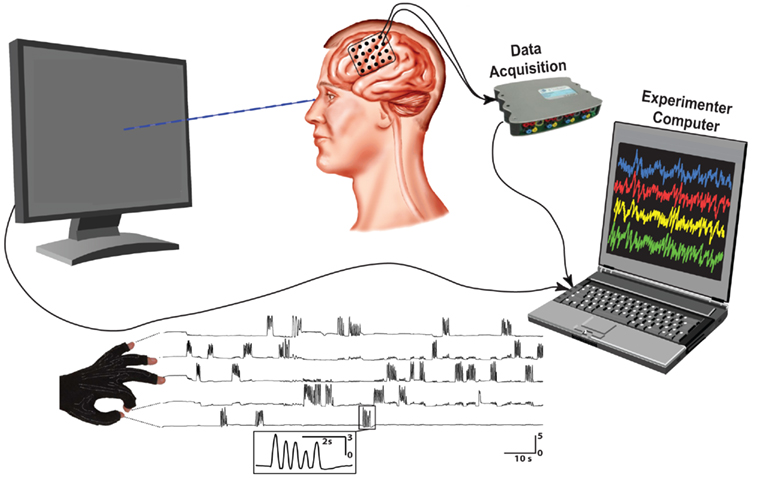
Figure 1. Experimental setup for this study.

The ECoG signals from the electrode grid were recorded using the general-purpose BCI2000 system (Schalk et al., 2004; Schalk and Mellinger, 2010) connected to a Neuroscan Synamps2 system. All electrodes were referenced to an inactive electrode that was far from the epileptogenic focus and areas of interest. The signals were further amplified, bandpass filtered between 0.15 and 200 Hz, and digitized at 1000 Hz. Each dataset was visually inspected and those channels that did not clearly contain ECoG activity (such as reference/ground electrodes) were removed, which resulted in 48, 63, 47, 64, and 61 channels (for subjects A–E respectively) for subsequent analyses.

2.2. Feature Extraction

Feature extraction was identical to that in (Kubánek et al., 2009). In short, we first re-referenced the signals using a common average reference (CAR), which subtracted from each channel, where H is the total number of channels and s_q is the collected signal at the qth channel and at the particular time. For each 100-ms time slice (overlapped by 50 ms) and each channel, we converted these time-series ECoG data into the frequency domain using an autoregressive model of order 20 (Marple, 1986). Using this model, we derived frequency amplitudes between 0 and 500 Hz in 1 Hz bins. ECoG features were extracted by averaging these frequency amplitudes across five frequency ranges, i.e., 8–12, 18–24, 75–115, 125–159, and 159–175 Hz. In addition to the frequency features described above, we obtained the Local Motor Potential (LMP; Schalk et al., 2007; Acharya et al., 2010) by averaging the raw time-domain signal at each channel over 100-ms time window. This resulted in 6 features for each of the ECoG channels, e.g., a total of 288 features from 48 channels.

2.3. Evaluation

We defined a movement period as the time between 1000 ms prior to movement onset and 1000 ms after movement offset. Movement onset was defined as the time when the finger’s flexion value exceeded an empirically defined threshold (one-fifth of the largest finger flexion value). Conversely, movement offset was defined as the time when the finger’s flexion value fell below that threshold and no movement onset was detected within the next 1200 ms (Kubánek et al., 2009). To achieve a dataset with relatively balanced movement and rest periods, we discarded all data outside the movement period. For each finger, we used fivefold cross validation to evaluate the performance of our modeling and inference algorithms that are described in more detail in the following sections, i.e., four-fifth of trials (around 30 trials and approximately 1320 ∼ 1650 samples) were used for training and one-fifth of trials were used for testing (around 5 trials and approximately 330 ∼ 420 data points). All analysis below were based on the output of pace regression (i.e., the same algorithm used in Kubánek et al., 2009), specifically the Pace Regression algorithm implemented in the Java-based Weka package (Hall et al., 2009), which estimated the time course of finger flexion from the time course of ECoG signal features.

3. Switching Non-Linear Dynamic System

The output of the pace regression algorithm was combined with prior knowledge using a switching non-linear dynamic system (SNDS). The SNDS is a Bayesian decoding model that infers the posterior distribution of finger flexion by combining a prior model and a measurement model (as shown in Figure 2). Similar regression/classification methods based on Bayesian inference have been adopted in a variety of domains (Viola and Jones, 2004; Tong et al., 2007; Yao et al., 2009; Taylor et al., 2010). In this work the prior model was represented by the structure and parameterizations of the SNDS, which were constructed to capture the constraints that govern the finger flexion. The measurement model was given by the output of pace regression, i.e., the prediction of finger flexion from the brain signal features.

FIGURE 2

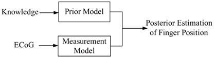
Figure 2. The schematic diagram of Bayesian decoding.

Section 3.1 develops a set of constraints that govern finger flexion. Section 3.2 then describes the construction of the prior model that incorporates these constraints. Section 3.3 discusses the measurement model. Finally, Section 3.4 describes learning and inference using SNDS.

3.1. Constraints that Govern Finger Flexion

In this section, we will develop a set of constraints that guide the movement of the fingers. These constraints commonly exist but are generally ignored by most decoding algorithms. Conventional decoding algorithms (such as pace regression) may make predictions that may be outside of these constraints. For example, a conventional decoding algorithms may produce a prediction of a finger that flexes past physical constraints, or may result in predictions in which a finger immediately proceeds from full extension to full flexion.

Figure 3 shows two examples of typical flexion traces. From this figure, we can make the following observations:

FIGURE 3

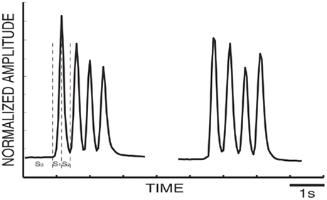
Figure 3. Examples of two flexion traces.

(i) The movement of fingers can be categorized into three states: extension (state S₁), flexion (state S₂), and rest (rest state S₃).

(ii) For each state, there are particular predominant movement patterns. In the extension state S₁, the finger keeps moving away from the rest position. In the flexion state S₂, the finger moves back to the rest position. In the rest state S₃, there are only very small movements.

(iii) For either state S₁ or state S₂, the movement speed is relatively low toward full flexion or full extension, but faster in between. For the rest state, the speed stays close to zero.

(iv) The natural flexion or extension of fingers are limited to certain ranges due to the physical constraints of our hand.

(v) The transition between different states is not random. Figure 4 shows the four possible transitions between three states. The extension state and flexion state can transfer to each other, while the rest state can only follow the flexion state and can only precede the extension state. This is also easy to understand from our common sense about natural finger flexion. When the finger is extended, it is impossible for it to directly transition into the rest state without experiencing flexion first. Similarly, fingers can not transition from the rest state to the flexion state without first going through the extension state.

(vi) Figure 4 discusses four possible ways of state transitions. The probability of these transitions depends on the finger position. For example, in the situation at hand, it is unlikely that the extension state transfers to the flexion state right after the extension state begins. At the same time, it is more likely to occur when the finger has extended enough and is near the end. Similar situations occur at other state transitions.

FIGURE 4

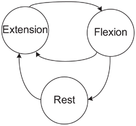
Figure 4. A diagram of possible state transitions for finger movements.

In summary, the observations described above provide constraints that govern finger flexion patterns. Using the methods described below, we will build a computational model that incorporates these constraints and that can systematically learn the movement patterns from data.

3.2. Prior Model

In this section, we show how the constraints summarized above are incorporated into the construction of the SNDS model. The SNDS is an extension of SLDS (Pavlovic et al., 2001; Oh et al., 2005) but with two key differences: (1) the continuous state transition is modeled by kernel density estimation to account for the speed changes under different finger positions; (2) the state not only depends on the previous state, but also the previous finger position. The prior model is shown as the top two layers in Figure 5. The top layer S represents moving states that include the extension state (S₁), flexion state (S₂), and rest state (S₃). The middle layer (continuous state variable) represents the real finger position. We discuss these two layers in detail below.

FIGURE 5

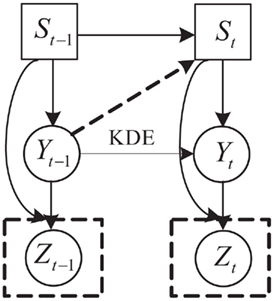
Figure 5. SNDS model in which S_t, Y_t, Z_t represent the moving states, real finger position, and the estimated finger position at time t, respectively.

3.2.1. State transitions (top layer)

In the standard SLDS, the probability of duration τ of state i is, according to the Markov assumption, defined as follows:

where q_ii denotes the transition probability of state i when it makes a self transition. Equation 1 states that the probability of staying in a given state decreases exponentially with time. This behavior can not provide an adequate representation for many natural temporal phenomena. The natural finger flexion is an example. It usually takes a certain amount of time for fingers to finish extension or flexion. Thus, the duration of certain movement patterns will deviate from the distribution described by Eq. 1.

This limitation of the state duration model has been addressed for hidden Markov models (HMMs) in the area of speech recognition by introducing explicit state duration distributions (Ferguson, 1980; Russell and Moore, 1985; Levinson, 1986; Ostendorf et al., 1996). In Ferguson (1980), duration was modeled by discrete probabilities. Later studies introduced parametric models, including the Gamma distribution (Levinson, 1986) and Poisson distribution (Russell and Moore, 1985). A similar idea was also introduced in switching linear dynamic system to form a segmental SLDS (Oh et al., 2008). While better performance was achieved, introducing state duration distribution complicates models as well as the learning and inference process. In fact, in many cases, the temporal variance is dependent on spatial variance, i.e., state transition is dependent on continuous state variables. In the context of finger flexion, as discussed in Section 3.1, the transition of moving states is dependent on finger position. In the model shown in Figure 5, the variable S_t not only has an incoming arrow from S_{t − 1} but also from Y_{t − 1}:

where P(Y_t−1|S_t−1) is a normalization term with no relation to S_t. P(S_t|S_t−1) is the state transition, which is same with that in HMM and standard SLDS. P(Y_t−1|S_t−1,S_t) is the posterior probability of Y_t−1 given state transition from S_t−1 to S_t. P(Y_t−1|S_t−1,S_t) plays a central role in controlling state transition. It directly relates state transition to finger position. We take the transition between extension state and flexion state as an example to give an intuitive explanation.

Figure 6A shows that the transition from extension state to flexion state most probably happens at the finger position between 1 and 2.5, which is near the extension end of movement. Similarly, Figure 6B implies that when the finger position is between −1.2 and −0.9, which is the flexion end of the finger movement, the transition from flexion state to extension state has a high probability.

FIGURE 6

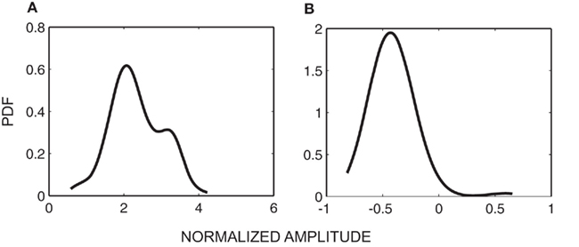
Figure 6. (A) Probabilistic density function (PDF) of Y_t−1 given S_t−1 = extension and S_t = flexion; (B) Probabilistic density function of Y_t−1 given S_t−1 = flexion and S_t = extension.

3.2.2. Continuous state transition (middle layer)

In SLDSs, the Y transition is linearly modeled. However, in our model, the continuous state transition is still highly non-linear during the extension and flexion states. This is mainly because the finger movement speed is uneven (fast in the middle but slow at the beginning and end). Modeling the continuous state transition properly is important for accurate decoding of finger movement. Here we propose a non-parametric method with which continuous state transitions are modeled using kernel density estimation (Frank et al., 2000). A Gaussian kernel is the most common choice because of its effectiveness and tractability (Marron and Wand, 1992). With a Gaussian kernel, the joint estimated joint distribution under each state can be obtained by:

where K(·) is a given kernel function; and are numeric bandwidth for Y_t−1 and Y_t. N is the total number of training examples. Our choice for K(·) is a Gaussian kernel Bandwidths and are estimated via a leave-one-out likelihood criterion (Loader, 1999), which maximizes:

where denotes the density estimated with (y_{i − 1},y_i) deleted. provides a much more accurate representation of continuous state transition than does a linear model.

Figure 7 gives an example of the kernel locations for under each of the three states (trained with part of the data from thumb flexion of subject A). Even though kernel locations do not represent the joint distribution , they do help to gain some insight into the relationship between Y_t−1 and Y_t. Each graph in Figure 7 describes a temporal transition pattern for each movement pattern. For the extension state, all kernel locations are above the diagonal, which means that statistically Y_t is greater than Y_t−1, i.e., fingers are moving up. Also the farther the kernel locations are from the diagonal, the larger the value of Y_t − Y_t−1, which implies greater moving speed at time t (because the time between t and t − 1 is a constant, Y_t − Y_t−1 could be a measurement of the speed). In the extension state, the moving speed around average flexion is statistically greater than that around the two extremes (full flexion and extension). Similar arguments can be applied to the flexion state in Figure 7. For the rest state, kernel locations are almost along the diagonal, which means Y_t = Y_t−1, i.e., fingers are not moving. The capability of being able to model the non-linear dependence of speed on position under each state is critical to make a precise prediction of the flexion trace.

FIGURE 7

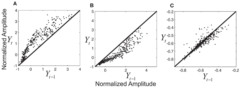
Figure 7. (A) Kernel locations for under extension state; (B) kernel locations for under flexion state; (C) kernel locations for under rest state. Numbers on the axis are the normalized amplitude of the fingers’ flexion.

3.3. Measurement Model (Bottom Layer)

Z in Figure 5 is the measurement, i.e., the time course of finger flexion predicted from ECoG using pace regression. Similar ways of constructing measurements as the output of other classifiers or regressors have been widely adopted in machine learning and computer vision community (Viola and Jones, 2004; Tong et al., 2007) as well as neural computation (Yao et al., 2009). Here we make an assumption that for each flexion pattern, Z_t depends linearly on Y_t, and is corrupted by Gaussian noise. Thus, this relationship can be represented by a linear Gaussian, which has been commonly used in Bayesian networks to accommodate continuous variables (Lauritzen, 1992; Friedman et al., 1998; Cowell et al., 2003). Specifically, we have

Parameters α^(s), μ^(s), and can be estimated from the training data via:

where E represents the statistical expectation and it is approximated by the sample mean.

3.4. Learning and Inference

3.4.1. Learning

All variables of the SNDS model are incorporated during learning. Finger flexion states are estimated from the behavioral flexion traces (e.g., Figure 3). Specifically, samples on the extension parts of the traces are labeled with state “extension,” samples on the flexion parts of the traces are labeled with state “flexion,” and samples during rest are labeled with state “rest.” Y is the true flexion trace, which we approximate with the data glove measurements.

All parameters in our model (Figure 5) consist of three components: the state transition parameter continuous state transition parameter and measurement parameter For state transition parameter as discussed in Eq. 2, P(S_t|S_t−1) and P(Y_t−1|S_t−1,S_t) are learned from the training data. P(S_t|S_t−1) can be simply obtained by counting. However, here we need to enforce the constraints described in Section 3.1(v). The elements in the conditional probability table of P(S_t|S_t−1) corresponding to the impossible state transitions are set to zero. P(Y_t−1|S_t−1,S_t) is estimated by kernel density estimation using the one-dimensional form of Eq. 1. Y transition parameter includes the joint distribution which can be estimated using Eq. 3 in which bandwidths were selected using the criteria in Eq. 4. includes α^(s), μ^(s), and and they can be estimated using Eqs 6–8.

3.4.2. Inference

Given the time course of ECoG signals, our goal is to infer the time course of finger flexion. This is a typical filtering problem, that is, recursively estimating the posterior distribution of S_t and Y_t given the measurement from the beginning to time t, i.e., Z_1:t:

where P(S_t−1,Y_t−1, Z_1:t) is the filtering result of the former step. However, we note that not all the continuous variables in our model follow a Gaussian distribution, because kernel density estimation was used to model the dynamics of the continuous state variable. Hence, it is infeasible to update the posterior distribution P(S_t,Y_t|Z_1:t) analytically in each step. To cope with this issue, we adopted a numerical sampling method based on particle filtering (Isard and Blake, 1998; Maskell and Gordon, 2001) to propagate and update the discretely approximated distribution over time. The inference algorithm is as follows:

(i) Initialization

• For t = 0 and i = 1,…,N, sample and from the initial distribution P(S₀) and P(Y₀|S₀).

(ii) Importance sampling

• For i = 1 to N, sample and from and .

• For i = 1 to N, evaluate the importance weights

• Normalize the importance weights:

(iii) Resampling

• For i = 1 to N, sample from the set according to the normalized importance weights .

Once the N samples and normalized importance weights have been constructed, the finger flexion at time step t can be estimated by:

where round(·) means rounding (·) to the nearest integers.

4. Results

4.1. Decoding of Finger Flexion Using Prior Knowledge

The main question we set out to answer in this study was to determine whether appropriate incorporation of prior knowledge can improve the performance of the decoding of finger flexion. We began our analyses by using SNDS in combination with a linear method (i.e., pace regression) as the underlying decoding algorithm. We previously used pace regression alone (i.e., without SNDS) to decode finger flexion using the same dataset (Kubánek et al., 2009).

To give a qualitative impression of the improvement of the SNDS algorithm combined with pace regression compared to pace regression alone, we first provide an example of the results achieved with each of these two approaches on the decoding of index finger flexion of subject A. These results are shown in Figure 8. In this figure, the top panel shows results achieved using pace regression and the middle figure shows results achieved using SNDS. In each of these two panels, the thin dotted line shows the actual flexion of the index finger (concatenated for five movement periods), and the thick solid line shows the flexion decoded using pace regression/SNDS. This figure demonstrates qualitatively that the decoding of finger flexion achieved using SNDS much better approximates the actual finger flexion than does pace regression. The bottom panel again shows the actual flexion pattern (thin dotted line) as well as the finger flexion state (1 = flexion, 2 = extension, 3 = rest; thick solid line).

FIGURE 8

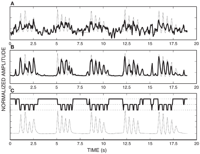
Figure 8. (A) Actual finger flexion (dotted trace) and decoded finger flexion (solid trace) using pace regression (mean square error 0.68); (B) Actual finger flexion (dotted trace) and decoded finger flexion (solid trace) using SNDS (mean square error 0.40); (C) Actual finger flexion (dotted trace) and state prediction (solid trace).

These results demonstrate that the state of finger flexion [which cannot be directly inferred using a method that does not incorporate a state machine (such as pace regression)] can be accurately inferred using SNDS.

In addition to the qualitative comparison provided above, Table 1 gives the main results of this study, which are a quantitative comparison between the results achieved using SNDS and pace regression. The results presented in this table are provided as mean squared error between actual and decoded finger flexion (min/max/mean, computed across cross validation folds). They show that for all fingers and all subjects, the results achieved using SNDS are superior to those achieved using pace regression alone. The overall mean square error reduces from 0.86 (pace regression) to 0.64 (SNDS), i.e., an improvement of 26%. This improvement of SNDS compared to pace regression was highly statistically significant (p << 0.001, paired t-test on the mean squared error for all fingers and subjects and between pace regression and SNDS).

TABLE 1

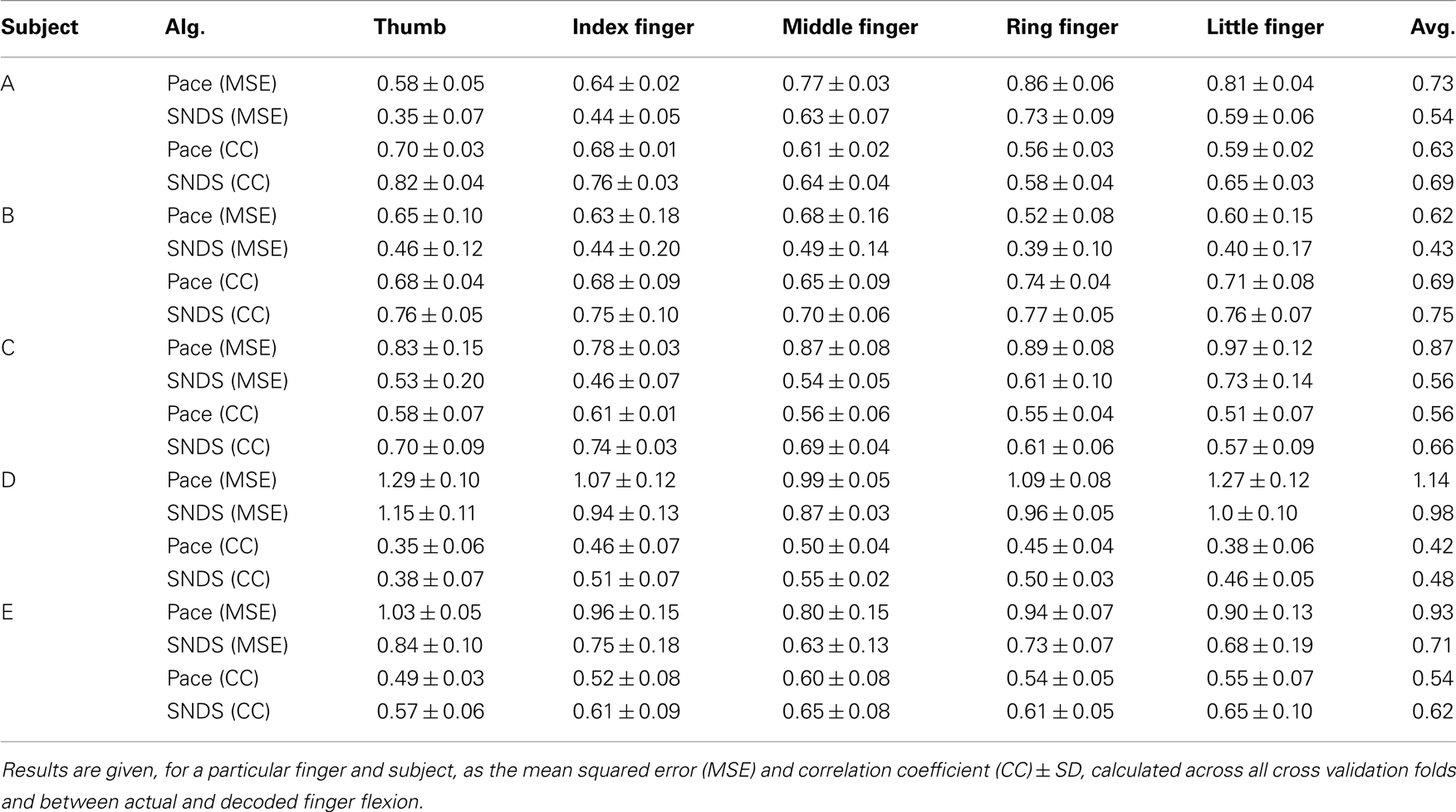
Table 1. Comparison of decoding performance between pace regression and SNDS.

4.2. Additional Analyses

4.2.1. Impact of different aspects of prior knowledge

The previous section demonstrated how we incorporated prior knowledge into a computational model to improve decoding of finger flexion. We were interested to what extent each aspect of the prior knowledge contributed to the improvement of the results. Thus, we incrementally incorporated each of these aspects into the model and determined the resulting effect.

The different models are shown in Figure 9. In this figure, the different models are: (a) a state-space model that captures the temporal dependency of finger flexion. The linear Gaussian in the state-space model can only capture linear transitions. (b) Introduces switch states that form a switched linear dynamic system (SLDS). Under SLDS, both the transition and measurement models are piecewise approximated using linear Gaussians. In other words, this version can model non-linear relationships to some extent. (c) Differs from (b) in that it replaces the linear Gaussian transition with the transition modeled by kernel density estimation. This refined transition can capture the dependency of movement speed on finger position and can constrain the finger movement range. Finally, (d) includes the dependency of state transition on the finger position by adding a link from Y_t−1 to S_t. The final model differs from the model (d) by replacing the linear Gaussian transition with kernel density estimation.

FIGURE 9

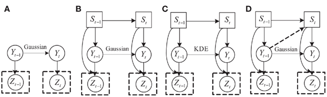
Figure 9. Comparison of computational models that incorporate different types of prior knowledge. See text for details.

Figure 10 shows the quantitative results in the mean squared error (also averaged across all fingers and subjects for each model). In addition, and similar to before, we ran a paired t-test between pace regression and SNDS for models (a–d), respectively, and all p-values were <<0.001. As mentioned above, these results show that the final model achieves a 26% reduction in mean squared error compared to pace regression. These quantitative improvements are also reflected in qualitative improvements in the decoded flexion traces: Figure 11 gives examples for decoded finger flexion traces using the different models. These results show that both model (a) (state-space model) and model (b) (SLDS) produce results that are quite improved compared to the results for pace regression. Figure 11 shows that the predicted flexion traces for model (a) are much smoother than those for pace regression, presumably due to the consideration of temporal correlations. The stronger descriptive power of model (b) provided by the state layer further improves on the results for model (a). Model (c) is produced by replacing the linear Gaussian transition with kernel density estimation in model (b). By refining the movement speed and constraining the movement range, model (c) produces accurate flexion traces as shown in Figure 11. Compared to the result of model (b), an obvious difference is that the flexion trace produced by model (c) stays relatively flat in the rest state. Model (d) provides another significant improvement by placing the dependency of state transition on the finger position, although this is not obvious in the short sample given in Figure 11. The final model, which combines elements from both (c) and (d), achieves results that are superior to both model (c) or model (d). The accurate finger flexion estimated by kernel density estimation allows for more accurate estimation of transitions, which in turn results in application of the correct kernel density estimation transition function, and thus results in improved finger flexion estimation.

FIGURE 10

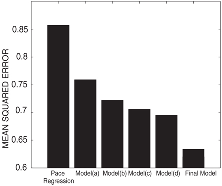
Figure 10. Performance (given as mean squared error for pace regression, intermediate models (a–d), and the final model.)

FIGURE 11

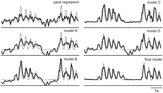
Figure 11. Exemplary decoding results of the models in Figure 10.

4.2.2. Using SNDS with a different decoding method

Because SNDS is a general probabilistic framework to incorporate prior knowledge into the decoding process, we also studied, as an example for the use of a different decoding algorithm, the combination of SNDS and a non-linear method (i.e., a Gaussian process Rasmussen, 1996). We previously used a Gaussian Process alone (i.e., without SNDS) to decode finger flexion using the same dataset (Wang et al., 2010).

The practical application of Gaussian processes is affected by its computational complexity, which is cubic to the data size. Sparse Gaussian processes (SPGP; Snelson and Ghahramani, 2006) have be developed to reduce its computational complexity. Table 2 shows the comparison for the four algorithms: pace regression, Gaussian process and SNDS combined with the output of pace regression and Gaussian process. For all subjects, the use of a Gaussian processes outperform the use of pace regression, and the use of SNDS outperformed the use of the respective decoding algorithm alone.

TABLE 2

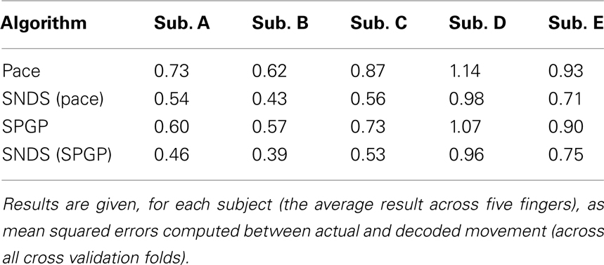
Table 2. Comparison of decoding performance between pace regression, Gaussian process, and SNDS using the output of these two algorithms.

5. Discussion

This paper demonstrates that prior knowledge can be successfully captured to build switched non-parametric dynamic systems to decode finger flexion from ECoG signals. We also showed that the resulting computational models improve the decoding of finger flexion compared to when prior knowledge was not incorporated. This improvement is possible by dividing the flexion activity into several moving states (S_t), considering the state transition over time, establishing specific state transition by considering its dependence on the finger position (continuous state variable Y_t) and modeling the individual transition pattern of continuous state variables under each moving state accurately by using kernel density estimation.

Generally, this improvements in decoding performance likely results from the different types of constraints on the possible flexion predictions that are realized by the computational model. In other words, the model may not able to produce all possible finger flexion patterns, although it is important to point out that the constraints that we put on finger flexions are those of natural finger flexions. Yet, it is still unclear to what extent these constraints and the same methodology used here may generalize to those of other natural movements, such as simultaneous movements of multiple fingers or hand gestures during natural reaches. In particular, our method improves results in part because it infers discrete behavioral states, but there may be many such states during natural movements, in particular when multiple degrees of freedom (e.g., movements of different fingers, wrist, hand, etc.) are considered. However, individual degrees of freedom of natural hand/finger movements are usually not independent, but are coordinated to form particular movement patterns such as those during reach-and-grasp. Thus, the number of possible states will usually be dramatically less than the number of all possible states. In this case, using techniques to reduce the dimensionality (such as principal component analysis, PCA) of the behavioral space should also limit the number of states. In other words, it would be straightforward to change the definition of states from movements of individual fingers to estimation of different grasp patterns. The general structure of the model would be the same while the parameterization and physical meanings of the variables would be somewhat different. At the same time, as the amount of prior knowledge decreases, e.g., movements along different degrees of freedom occur unpredictably and independently, the benefit of using prior knowledge will likely decrease.

There are some directions in which this work could be further improved. First, to reduce the computational complexity caused by kernel density estimation, non-linear transition functions can be used to model the continuous state transitions. Second, more efficient inference methods could be developed to replace standard particle sampling. Finally, the methods presented in this paper could be extended to allow for simultaneous decoding of all five fingers instead of one at a time.

In conclusion, the results presented in this paper demonstrate that, with appropriate mathematical decoding algorithms, ECoG signals can give information about finger movements that in their specificity and fidelity goes substantially beyond what has previously been demonstrated using any other method in any species. With further improvements to current ECoG sensor technology, in particular to the density and form factor of current implants, and extension of current methods to real-time capability, it may ultimately be possible to develop neurally controlled hand prostheses with full fine-grained finger articulation. This eventual prospect is exciting, because even simpler capabilities may offer distinct advantages, e.g., the restoration of select grasp patterns in stroke patients. More generally, the possibility that ECoG may support practical, robust, and chronic brain–computer interfaces was recently further substantiated: the study by Chao et al. (2010) showed that the signal-to-noise ratio of ECoG signals, and the cortical representations of motor functions that can be identified with ECoG, are stable over several months (Schalk, 2010).

Conflict of Interest Statement

The authors declare that the research was conducted in the absence of any commercial or financial relationships that could be construed as a potential conflict of interest.

Acknowledgments

This work was supported in part by grants from the US Army Research Office [W911NF-07-1-0415 (Gerwin Schalk) and W911NF-08-1-0216 (Gerwin Schalk)] and the NIH [EB006356 (Gerwin Schalk) and EB000856 (Gerwin Schalk)].

References

Acharya, S., Fifer, M. S., Benz, H. L., Crone, N. E., and Thakor, N. V. (2010). Electrocorticographic amplitude predicts finger positions during slow grasping motions of the hand. J. Neural Eng. 7, 046002.

Pubmed Abstract | Pubmed Full Text | CrossRef Full Text

Azzouzi, M., and Nabney, I. T. (1999). “Modelling financial time series with switching state space models,” in Proceedings on IEEE/IAFE 1999 Conference on Computational Intelligence for Financial Engineering, Port Jefferson, NY: Institute of Electrical and Electronics Engineers (IEEE), 240C249.

Bashashati, A., Fatourechi, M., Ward, R. K., and Birch, G. E. (2007). A survey of signal processing algorithms in brain-computer interfaces based on electrical brain signals. J. Neural Eng. 4, R32–R57.

Pubmed Abstract | Pubmed Full Text | CrossRef Full Text

Bradberry, T. J., Gentili, R. J., and Contreras-Vidal, J. L. (2010). Reconstructing three-dimensional hand movements from noninvasive electroencephalographic signals. J. Neurosci. 30, 3432–3437.

Pubmed Abstract | Pubmed Full Text | CrossRef Full Text

Bradberry, T. J., Gentili, R. J., and Contreras-Vidal, J. L. (2011). Fast attainment of computer cursor control with noninvasively acquired brain signals. J. Neural Eng. 8, 036010.

Pubmed Abstract | Pubmed Full Text | CrossRef Full Text

Carmena, J. M., Lebedev, M. A., Henriquez, C. S., and Nicolelis, M. A. L. (2005). Stable ensemble performance with single-neuron variability during reaching movements in primates. J. Neurosci. 25, 10712–10716.

Pubmed Abstract | Pubmed Full Text | CrossRef Full Text

Chao, Z. C., Nagasaka, Y., and Fujii, N. (2010). Long-term asynchronous decoding of arm motion using electrocorticographic signals in monkeys. Front. Neuroeng. 3:3. doi: 10.3389/fneng.2010.00003

CrossRef Full Text

Chapin, J. K., Moxon, K. A., Markowitz, R. S., and Nicolelis, M. A. (1999). Real-time control of a robot arm using simultaneously recorded neurons in the motor cortex. Nat. Neurosci. 2, 664–670.

Pubmed Abstract | Pubmed Full Text | CrossRef Full Text

Cowell, R. G., Dawid, P. A., Lauritzen, S. L., and Spiegelhalter, D. J. (2003). Probabilistic Networks and Expert Systems (Information Science and Statistics). New York: Springer.

Droppo, J., and Acero, A. (2004). “Noise robust speech recognition with a switching linear dynamic model,” in Acoustics, Speech, and Signal Processing, 2004. Proceedings. (ICASSP’04). IEEE International Conference on, Vol. 1, Montreal, I–953–6.

Ferguson, J. (1980). “Variable duration models for speech,” in Proc. of the Symposium on the Application of Hidden Markov Models to Text and Speech, Princeton, NJ, 143–179.

Frank, E., Trigg, L., Holmes, G., Witten, I. H., and Aha, W. (2000). “Naive Bayes for regression,” in Machine Learning, Boston: Kluwer Academic Publishers, 5–26.

Friedman, N., Goldszmidt, M., and Lee, T. J. (1998). “Bayesian network classification with continuous attributes: getting the best of both discretization and parametric fitting,” in Proceedings of the International Conference on Machine Learning (ICML) (San Francisco, CA: Morgan Kaufmann), 179–187.

Hall, M., Frank, E., Holmes, G., Pfahringer, B., Reutemann, P., and Witten, I. H. (2009). The WEKA data mining software: an update. SIGKDD Explor. Newsl. 11, 10–18.

CrossRef Full Text

Hatsopoulos, N., Joshi, J., and O’Leary, J. G. (2004). Decoding continuous and discrete motor behaviors using motor and premotor cortical ensembles. J. Neurophysiol. 92, 1165–1174.

Pubmed Abstract | Pubmed Full Text | CrossRef Full Text

Isard, M., and Blake, A. (1998). Condensation – conditional density propagation for visual tracking. Int. J. Comput. Vis. 29, 5–28.

CrossRef Full Text

Kim, K. H., Kim, S. S., and Kim, S. J. (2006). Superiority of nonlinear mapping in decoding multiple single-unit neuronal spike trains: a simulation study. J. Neurosci. Methods 150, 202–211.

Pubmed Abstract | Pubmed Full Text | CrossRef Full Text

Kim, S.-P., Rao, Y. N., Erdogmus, D., Sanchez, J. C., Nicolelis, M. A. L., and Principe, J. C. (2005). Determining patterns in neural activity for reaching movements using nonnegative matrix factorization. EURASIP J. Appl. Signal Process. 2005, 3113–3121.

CrossRef Full Text

Koyama, S., Chase, S. M., Whitford, A. S., Velliste, M., Schwartz, A. B., and Kass, R. E. (2010). Comparison of brain-computer interface decoding algorithms in open-loop and closed-loop control. J. Comput. Neurosci. 29, 73–87.

Pubmed Abstract | Pubmed Full Text | CrossRef Full Text

Kubánek, J., Miller, K. J., Ojemann, J. G., Wolpaw, J. R., and Schalk, G. (2009). Decoding flexion of individual fingers using electrocorticographic signals in humans. J. Neural Eng. 6, 066001.

Pubmed Abstract | Pubmed Full Text | CrossRef Full Text

Lauritzen, S. L. (1992). Propagation of probabilities, means, and variances in mixed graphical association models. J. Am. Stat. Assoc. 87, 1098–1108.

CrossRef Full Text

Lebedev, M. A., Carmena, J. M., O’Doherty, J. E., Zacksenhouse, M., Henriquez, C. S., Principe, J. C., and Nicolelis, M. A. L. (2005). Cortical ensemble adaptation to represent velocity of an artificial actuator controlled by a brain-machine interface. J. Neurosci. 25, 4681–4693.

Pubmed Abstract | Pubmed Full Text | CrossRef Full Text

Levinson, S. (1986). “Continuously variable duration hidden Markov models for speech analysis,” in Acoustics, Speech, and Signal Processing, IEEE International Conference on ICASSP’86, Vol. 11, Tokyo, 1241–1244.

Loader, C. R. (1999). Bandwidth selection: classical or plug-in? Ann. Stat. 27, 415–438.

CrossRef Full Text

Lotte, F., Congedo, M., Lécuyer, A., Lamarche, F., and Arnaldi, B. (2007). A review of classification algorithms for EEG-based brain-computer interfaces. J. Neural Eng. 4, 1–1.

Pubmed Abstract | Pubmed Full Text | CrossRef Full Text

Marple, S. L. (1986). Digital Spectral Analysis: With Applications. Upper Saddle River, NJ: Prentice-Hall, Inc.

Marron, J. S., and Wand, M. P. (1992). Exact mean integrated squared error. Ann. Stat. 20, 712–736.

CrossRef Full Text

Maskell, S., and Gordon, N. (2001). A tutorial on particle filters for on-line nonlinear/non-Gaussian Bayesian tracking. IEEE Trans. Signal Process. 50, 174–188.

McFarland, D. J., Krusienski, D. J., Sarnacki, W. A., and Wolpaw, J. R. (2008). Emulation of computer mouse control with a noninvasive brain-computer interface. J. Neural Eng. 5, 101–110.

Pubmed Abstract | Pubmed Full Text | CrossRef Full Text

McFarland, D. J., Sarnacki, W. A., and Wolpaw, J. R. (2010). Electroencephalographic EEG control of three-dimensional movement. J. Neural Eng. 7, 036007.

Pubmed Abstract | Pubmed Full Text | CrossRef Full Text

Muller, K.-R., Anderson, C., and Birch, G. (2003). Linear and nonlinear methods for brain-computer interfaces. IEEE Trans. Neural Syst. Rehabil. Eng. 11, 165–169.

Pubmed Abstract | Pubmed Full Text | CrossRef Full Text

Mulliken, G. H., Musallam, S., and Andersen, R. A. (2008). Decoding trajectories from posterior parietal cortex ensembles. J. Neurosci. 28, 12913–12926.

Pubmed Abstract | Pubmed Full Text | CrossRef Full Text

Oh, S. M., Rehg, J., Balch, T., and Dellaert, F. (2005). “Learning and inference in parametric switching linear dynamic systems,” in Computer Vision, 2005. ICCV 2005. Tenth IEEE International Conference on, Vol. 2, Beijing, 1161–1168.

Oh, S. M., Rehg, J. M., Balch, T., and Dellaert, F. (2008). Learning and inferring motion patterns using parametric segmental switching linear dynamic systems. Int. J. Comput. Vis. 77, 103–124.

CrossRef Full Text

Ostendorf, M., Digalakis, V., and Kimball, O. (1996). From HMM’s to segment models: a unified view of stochastic modeling for speech recognition. IEEE Trans. Speech Audio Process. 4, 360–378.

CrossRef Full Text

Pavlovic, V., Rehg, J. M., and MacCormick, J. (2001). Learning switching linear models of human motion. Adv. Neural Inf. Process Syst. 2000, 981–987.

Presacco, A., Goodman, R., Forrester, L. W., and Contreras-Vidal, J. L. (2011). Neural decoding of treadmill walking from non-invasive, electroencephalographic (EEG) signals. J. Neurophysiol. doi: 10.1152/jn.00104.2011. [Epub ahead of print].

CrossRef Full Text

Rasmussen, C. E. (1996). Evaluation of Gaussian Processes and Other Methods for Non-Linear Regression. Technical Report, University of Toronto, Toronto.

Rosti, A. V. I., and Gales, M. (2004). “Rao-blackwellised Gibbs sampling for switching linear dynamical systems,” in IEEE International Conference on Acoustics, Speech, and Signal Processing (ICASSP 2004), Montreal, 809–812.

Russell, M., and Moore, R. (1985). “Explicit modelling of state occupancy in hidden Markov models for automatic speech recognition,” in Acoustics, Speech, and Signal Processing, IEEE International Conference on ICASSP’85, Vol. 10, Tampa, FL, 5–8.

Sanchez, J., Erdogmus, D., Rao, Y., Principe, J., Nicolelis, M., and Wessberg, J. (2003). “Learning the contributions of the motor, premotor, and posterior parietal cortices for hand trajectory reconstruction in a brain machine interface,” in Neural Engineering, 2003. Conference Proceedings. First International IEEE EMBS Conference on, Cancun, 59–62.

Sanchez, J. C., Erdogmus, D., and Principe, J. C. (2002). “Comparison between nonlinear mappings and linear state estimation to model the relation from motor cortical neuronal firing to hand movements,” in Proceedings of SAB Workshop on Motor Control in Humans and Robots: On the Interplay of Real Brains and Artificial Devices, Edinburgh, 59–65.

Schalk, G. (2010). Can electrocorticography (ECoG) support robust and powerful brain-computer interfaces? Front. Neuroeng. 3:9. doi: 10.3389/fneng.2010.00009

Pubmed Abstract | Pubmed Full Text | CrossRef Full Text

Schalk, G., Kubánek, J., Miller, K. J., Anderson, N. R., Leuthardt, E. C., Ojemann, J. G., Limbrick, D., Moran, D., Gerhardt, L. A., and Wolpaw, J. R. (2007). Decoding two-dimensional movement trajectories using electrocorticographic signals in humans. J. Neural Eng. 4, 264–275.

Pubmed Abstract | Pubmed Full Text | CrossRef Full Text

Schalk, G., McFarland, D. J., Hinterberger, T., Birbaumer, N., and Wolpaw, J. R. (2004). BCI2000: a general-purpose brain-computer interface (BCI) system. IEEE Trans. Biomed. Eng. 51, 1034–1043.

Pubmed Abstract | Pubmed Full Text | CrossRef Full Text

Schalk, G., and Mellinger, J. (2010). A Practical Guide to Brain-Computer Interfacing with BCI2000. New York, NY: Springer-Verlag.

Schwartz, A. B., Taylor, D. M., and Tillery, S. I. (2001). Extraction algorithms for cortical control of arm prosthetics. Curr. Opin. Neurobiol. 11, 701–707.

Pubmed Abstract | Pubmed Full Text | CrossRef Full Text

Snelson, E., and Ghahramani, Z. (2006). Sparse Gaussian processes using pseudo-inputs. Adv. Neural Inf. Process. Syst. 18, 1257–1264.

Taylor, D. M., Tillery, S. I., and Schwartz, A. B. (2002). Direct cortical control of 3D neuroprosthetic devices. Science 296, 1829–1832.

Pubmed Abstract | Pubmed Full Text | CrossRef Full Text

Taylor, G., Sigal, L., Fleet, D., and Hinton, G. (2010). “Dynamical binary latent variable models for 3d human pose tracking,” in Computer Vision and Pattern Recognition (CVPR), 2010 IEEE Conference on, San Francisco, CA, 631–638.

Taylor, G. W., Hinton, G. E., and Roweis, S. (2006). Modeling human motion using binary latent variables. Adv. Neural Inf. Process. Syst. 19, 1345.

Tong, Y., and Ji, Q. (2008). “Learning Bayesian networks with qualitative constraints,” in CVPR 2008. IEEE Conference on, Anchorage, 1–8.

Tong, Y., Liao, W., and Ji, Q. (2007). Facial action unit recognition by exploiting their dynamic and semantic relationships. IEEE Trans. Pattern Anal. Mach. Intell. 29, 1683–1699.

Pubmed Abstract | Pubmed Full Text | CrossRef Full Text

Velliste, M., Perel, S., Spalding, M. C., Whitford, A. S., and Schwartz, A. B. (2008). Cortical control of a prosthetic arm for self-feeding. Nature 453, 1098–1101.

Pubmed Abstract | Pubmed Full Text | CrossRef Full Text

Viola, P., and Jones, M. (2004). Robust real-time face detection. Int. J. Comput. Vis. 57, 137–154.

CrossRef Full Text

Wang, Z., Ji, Q., Miller, K., and Schalk, G. (2010). “Decoding finger flexion from electrocorticographic signals using a sparse Gaussian process,” in Proceedings of the 2010 20th International Conference on Pattern Recognition, ICPR’10 (Washington, DC: IEEE Computer Society), 3756–3759.

Wolpaw, J. R. (2007). “Brain-computer interfaces (BCIs) for communication and control,” in Proceedings of the 9th international ACM SIGACCESS conference on Computers and accessibility, Assets’07 (New York, NY: ACM), 1–2.

Wolpaw, J. R., and McFarland, D. J. (2004). Control of a two-dimensional movement signal by a noninvasive brain-computer interface in humans. Proc. Natl. Acad. Sci. U.S.A. 101, 17849–17854.

Pubmed Abstract | Pubmed Full Text | CrossRef Full Text

Yao, B., Walther, D., Beck, D., and Fei-Fei, L. (2009). “Hierarchical mixture of classification experts uncovers interactions between brain regions,” in Annual Conference on Neural Information Processing Systems (NIPS) (Vancouver: NIPS).

Zoeter, O., and Heskes, T. (2003). Hierarchical visualization of time-series data using switching linear dynamical systems. IEEE Trans. Pattern Anal. Machine Intell. 25, 1202–1214.

CrossRef Full Text