Emergent Auditory Feature Tuning in a Real-Time Neuromorphic VLSI System

Many sounds of ecological importance, such as communication calls, are characterized by time-varying spectra. However, most neuromorphic auditory models to date have focused on distinguishing mainly static patterns, under the assumption that dynamic patterns can be learned as sequences of static ones. In contrast, the emergence of dynamic feature sensitivity through exposure to formative stimuli has been recently modeled in a network of spiking neurons based on the thalamo-cortical architecture. The proposed network models the effect of lateral and recurrent connections between cortical layers, distance-dependent axonal transmission delays, and learning in the form of Spike Timing Dependent Plasticity (STDP), which effects stimulus-driven changes in the pattern of network connectivity. In this paper we demonstrate how these principles can be efficiently implemented in neuromorphic hardware. In doing so we address two principle problems in the design of neuromorphic systems: real-time event-based asynchronous communication in multi-chip systems, and the realization in hybrid analog/digital VLSI technology of neural computational principles that we propose underlie plasticity in neural processing of dynamic stimuli. The result is a hardware neural network that learns in real-time and shows preferential responses, after exposure, to stimuli exhibiting particular spectro-temporal patterns. The availability of hardware on which the model can be implemented, makes this a significant step toward the development of adaptive, neurobiologically plausible, spike-based, artificial sensory systems.

1. Introduction

Hardware implementations of neuromorphic systems (Indiveri and Horiuchi, 2011) have been successfully used in the past to implement and characterize biophysically realistic models of the early sensory processing stages both for the visual domain (Koch and Mathur, 1996; Liu, 1999; Barbaro et al., 2002; Kramer, 2002; Culurciello et al., 2003; Lichtsteiner et al., 2006; Zaghloul and Boahen, 2006; Leñero-Bardallo et al., 2010), and the auditory domain (Watts et al., 1992; Toumazou et al., 1994; van Schaik et al., 1996; Fragnière et al., 1997; van Schaik and Meddis, 1999; Wen and Boahen, 2006; Chan et al., 2007; Abdalla and Horiuchi, 2008). These systems were typically implemented as single Very Large Scale Integration (VLSI) devices (e.g., as silicon retinas, or silicon cochleas), comprising hybrid analog/digital circuits that faithfully reproduced in real-time the bio-physics of the neural sensory systems they modeled. The definition of an event (spike) based communication protocol based on the Address Event Representation (AER; Deiss et al., 1999; Boahen, 2000) has led to the development of a new generation of more complex multi-chip neuromorphic sensory systems (Liu et al., 2001; Choi et al., 2005; Chicca et al., 2007; Folowosele et al., 2008; Serrano-Gotarredona et al., 2009). However, while it is now possible to build hardware sensory systems that can react to auditory and visual stimuli, and eventually drive robotic actuators in real-time (see for example the exciting projects being developed at the Telluride¹ and Capo Caccia Neuromorphic Engineering workshops², it still remains a challenge to build real-time sensory processing systems that can learn about the nature of their input stimuli and perform cognitive tasks, using spikes and spiking neural networks.

There are two main bottlenecks that have been hindering progress in this area: one has to do with the practical difficulties of linking real-time asynchronous neuromorphic devices to each-other to build complex multi-chip systems; and the other is related to the theoretical and computational challenges in integrating and extracting information from the time-varying signals representing inputs, outputs, and internal state variables, in these types of systems.

The first problem, that of developing real-time interfaces between the different AER chips to create complex multi-chip systems, is currently being addressed by developing both custom real-time hardware solutions (Gomez-Rodriguez et al., 2006; Fasnacht et al., 2008; Hofstaetter et al., 2010; Jin et al., 2010; Fasnacht and Indiveri, 2011; Scholze et al., 2011), as well as software solutions, and principled systematic methods for configuring network structures and system parameters (Davison et al., 2008; Neftci et al., 2011, 2012; Sheik et al., 2011).

The second problem is more fundamental. There is, in general, agreement that cells in primary sensory areas are typically characterized in terms of tuning to particular spectro-temporal features³. It is not, however, clear what features are encoded, or what neural mechanisms underlie those feature selectivities, or what developmental processes lead to the formation of those mechanisms. Although pursuing these questions has led to remarkable advances in understanding visual processing in the brain, a corresponding understanding of auditory processing is still lacking.

Here we present a multi-chip neuromorphic system in which silicon neurons (Indiveri et al., 2011) dynamically adapt and learn, forming feature tuning properties that are derived from spectro-temporal correlations in their input spike trains. The auditory domain was chosen as the focus for the experiments, where the importance of dynamic spectro-temporal patterns in the communication calls of mammals and birds has motivated the study of cortical sensitivity to frequency sweeps (Godey et al., 2005; Atencio et al., 2007; Ye et al., 2010) and dynamic ripple noises (Kowalski et al., 1996; Calhoun and Schreiner, 1998; Depireux et al., 2001; Atencio and Schreiner, 2010) as candidates for constituent features which are sufficiently simple to be parametrized.

The multi-chip neuromorphic system implements a neural network model of the auditory thalamo-cortical system similar to that described in Coath et al. (2011). We demonstrate that this system can learn, when repeatedly presented with a specific stimulus, to exhibit a preferential response to such a stimulus. We argue that the functional principles of this neural network, and of the thalamo-cortical model (Coath et al., 2011) it is derived from, can be used to produce spike-based feature extractors and that these could form the basis of artificial sensory systems using real-time analog neuromorphic VLSI.

2. Materials and Methods

2.1. Network Model

The structure of the neural network implemented in hardware is shown in Figure 1. It comprises three populations of neurons, one A population and two B populations (B₁ and B₂), arranged tonotopically. The A neurons are implemented in software and provide spikes that represent the input auditory signals.

FIGURE 1

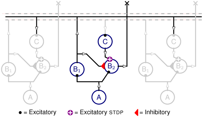
Figure 1. Neural network diagram, with one column highlighted and two neighboring ones in gray, included to indicate lateral connections. Circles represent neurons from neuronal populations A, B₁, B₁, and C. Auditory input signals are produced by the tonotopically arranged neurons in populations A (implemented in software). The spikes produced by A are projected onto both populations B₁ and B₂. Neurons in B₂ also receive inhibitory inputs from B₁ neurons, as well as recurrent excitation from B₁ neurons of neighboring units via delay neurons C, and STDP synapses. The output of the network is represented by the activity of population B₂.

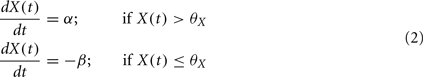
Each A neuron projects to a B₁ and a B₂ neuron via excitatory synapses, the B₁ neurons project to B₂ neurons via inhibitory synapses, and the B₁ neurons project, via the intermediate C population, onto their neighboring B₂ neurons. The C neurons implement the propagation delays as described in Section 2.3 and the C to B₂ projections are mediated by excitatory plastic synapses which are the loci of the Spike Timing Dependent Plasticity (STDP) as described in Section 2.4.

The propagation delays (that is the time it takes for a spike to travel from B₁ to reach B₂) are proportional to the tonotopic distance between pre-synaptic and post-synaptic neurons (see Figure 4). The plastic synapses from C to B₂ perform the key task of learning the temporal correlations in the time-varying stimulus.

When neurons in population A spike, they produce Excitatory Post-Synaptic Potential (EPSPs) in the B populations. The synapses from A to B₁ neurons have slightly higher weights than those that project to the B₂ neurons. Therefore, in spite of being driven by the same A activity, B₁ neurons spike slightly before B₂ ones. The inhibitory projections are used to ensure that B₂ neurons remain silent as long as the delayed projections are not potentiated. When a stimulus, the (exposure stimulus (ES)), is presented repeatedly to the network, the B₁ neurons fire stereotypically, following the input from A neurons. The delayed feedback reaches B₂ neurons at different times after stimulus onset. The correlation between this delayed feedback and the membrane potential of B₂ neurons causes the plastic synapses to potentiate or depress. When a pre-synaptic spike reaches the post-synaptic neuron while its membrane is close to its firing threshold, the synapse is potentiated, otherwise the synapse is depressed. The details of the STDP update rule are explained in Section 2.4.

Once the network has learned the ES, the output current of the potentiated STDP synapses overcomes the inhibition reaching B₂ neurons and makes them fire; but this is effective only when the spikes at these synapses arrive before the inhibition takes effect. This causes the B₂ neurons to be active only when the right stimulus ES is presented and therefore, the activity of B₂ neurons can be used as an effective readout. A simple spike count from B₂ neurons is sufficient to discriminate the ES from any other stimuli.

2.2. The Hardware Implementation

The hardware implementation of the network model consists of a real-time multi-chip setup, as shown in Figure 2. It consists of three multi-neuron spiking chips and an AER mapper (Fasnacht and Indiveri, 2011) connected in a serial loop. The multi-neuron chips were fabricated using a standard AMS 0.35 μm CMOS process. Two of the three multi-neuron chips (CHIP–1 and CHIP–2) are identical and comprise an array of 128 linear integrate-and-fire neurons (Indiveri et al., 2006) and 128 × 32 synaptic circuits. Each neuron in the chip is connected to 2 excitatory, 2 inhibitory, and 28 excitatory plastic synapse circuits.

FIGURE 2

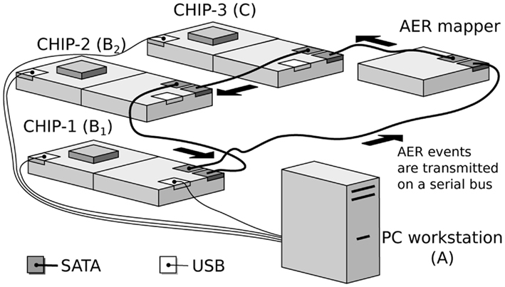
Figure 2. Real-time multi-chip setup. The chips are mounted on custom PCBs (AMDA) which supply bias voltages to the chips. These biases can be configured via a USB interface connected to the PC workstation. The AER events are handled by dedicated PCBs equipped with FPGAs (AEX; Fasnacht et al., 2008). These events are transmitted from one board to the other over SATA cables in a serial loop. Events can also be sent and monitored from a PC workstation via a USB interface.

These chips are also equipped with a synapse multiplexer, which enables a neuron to redirect synaptic currents from neighboring rows onto itself. This allows the use of more synapses per neuron, at the cost of using fewer neurons in total. Depending on the multiplexer configuration it is possible to achieve combinations of synapse and neuron numbers, ranging from 128 neurons each with 32 synapses, to 1 neuron with 4096 synapses.

The third multi-neuron chip (CHIP–3) comprises a two-dimensional array of 32-by-64 neurons. Each neuron in the chip is connected to 3 synaptic circuits (2 excitatory, 1 inhibitory).

The excitatory and inhibitory synapse circuits on all three chips, which implement their temporal dynamics, are based on the current-mode Differential-Pair Integrator (DPI) circuit proposed in Bartolozzi and Indiveri (2007). These synapses produce Excitatory Post-Synaptic Current (EPSCs) and Inhibitory Post-Synaptic Current (IPSCs) respectively with realistic temporal dynamics on the arrival of a pre-synaptic input spike.

The AER mapper allows the implementation of a wide range of neural network topologies including multi-layer networks and fully recurrent networks. The topology is defined by programming a look-up table that the AER mapper reads to route spikes from source neurons to destination synapses. The network topology of Figure 1 was obtained by mapping the populations B₁ and B₂ onto CHIP–1 and CHIP–2 respectively. The synapse multiplexers on CHIP–1 and CHIP–2 were configured to have 32 active neurons with 128 input synapses each, 112 of which are plastic. Each neuron in B₁ was connected to a neuron in B₂ using three plastic synapses. The use of multiple redundant synapses is helpful in reducing the effect of device mismatch in the plastic synapse circuits by ensuring that at least a fraction of these synapses exhibit the desired dynamics. Neurons from CHIP–3 were used to implement the population C, which implement delayed feedback to B₂ neurons.

2.3. Delayed Feedback

The current hardware does not directly support propagation delays between neurons. To overcome this limitation, long synaptic and neuronal time constants are exploited. Given that the weights associated with the synapses of a neuron are strong enough to produce a single output spike, the time difference between the pre-synaptic spike and the post-synaptic spike is considered equivalent to propagation/transmission delay. Therefore, every projection in the model that requires a delay is passed through an additional neuron, referred to as a delay neuron. The delay neurons are labeled C in Figure 1.

The transmission delay of a delay neuron is a function of synaptic strength, synaptic and neuronal time constants and firing threshold. Delays of the order of milliseconds can be achieved by setting a weak synaptic strength and a long time constant, to produce a long-lasting small output current. In this configuration, synaptic circuits are strongly affected by transistor mismatch and as a result they produce a broad distribution of output currents, despite sharing global biases. These output currents, integrated by the post-synaptic neurons, produce output spikes with a broad distribution of delays from the input spikes. Depending on the required delay, an appropriate delay neuron is selected and placed in the network.

Figure 3 shows the distribution of delays across 1070 neurons on CHIP–3 for a specific configuration of biases. The delays range from 0.7 to 8.6 ms with a mean of approximately 2.5 ms. Although the chip contains 2048 neurons, because of device mismatch, only a subset of these neurons can be used as delay neurons. The rest of the neurons either have too strong or too weak synaptic strength, causing the neurons to fire multiple or no spikes per incoming spike.

FIGURE 3

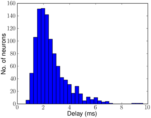
Figure 3. Histogram of delays of 1070 of the 2048 neurons on CHIP–3 due to mismatch in the hardware. Delays range from 0.7 to 8.6 ms mean ≈2.5 ms. The remaining neurons either fire more than once or not at all.

2.4. The STDP Update Rule

The network model includes excitatory projections from C to B₂ which are plastic and exhibit STDP, a spike-based Hebbian learning rule (Caporale and Dan, 2008). The synaptic weight is incremented when the pre-synaptic spike arrives before the post-synaptic spike, and decremented if the order is reversed; hence this rule potentiates those synapses where an apparent cause-effect relationship predominates over time.

A modified version of the STDP rule is implemented in analog VLSI on the plastic synapses of neuromorphic chips (1, 2) used in this experiment (Giulioni et al., 2009; Mitra et al., 2009). The synaptic update rule (Brader et al., 2007) adjusts the synaptic weight, or efficacy, X upon arrival of a pre-synaptic spike, depending on the instantaneous membrane potential and the internal state of the post-synaptic neuron (Fusi, 2003; Brader et al., 2007). The internal state, C(t), is putatively identified with the post-synaptic neuron calcium concentration, driven by firing of the neuron (Shouval et al., 2002).

The synaptic efficacy, X, is altered according to rules given in Equation 1. If at the time of arrival of a pre-synaptic spike the post-synaptic membrane voltage, V(t), is high (above threshold þ) and its internal state C(t) is within the bounds [], then the synaptic efficacy is increased by an amount, a. On the other hand if V(t) is low (below the learning threshold þ) and C(t) is within the bounds [], then the synaptic efficacy is decreased by an amount b:

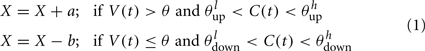
If neither of the conditions is satisfied, then X drifts to one of two stable states 0 or 1, depending on whether X(t) is above or below the threshold, þ_X:

The internal state, C(t), is driven by firing of the neuron and is governed by:

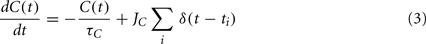
where J_C is the amount of calcium contributed by a single spike.

2.5. Input Stimuli

Examples of the spiking inputs, which were used as the ES and probe stimulus (PS) signals, are shown in Figure 5. Figure 5A illustrates a single linear frequency sweep, while Figure 5B shows an example of the second class of stimuli (forked), with a diverging pattern of activity. The stimuli of the second type are essentially a combination of two frequency sweeps, one increasing and one decreasing. We use examples of both types of stimuli with a range of FM seep velocities. The velocity in each case is given as the number of channels activated per millisecond, for example Figure 5A shows an upward sweep with the onset of activity in each channel separated by 1 ms, hence the velocity is +1.0 ms⁻¹. Downward sweeps have negative velocities, and in the case of the forked stimuli the velocity of the component in the upper half of the is axis is given.

The differences in the spike patterns in each channel shown in Figure 5 are systematically introduced to compensate for the device mismatch effects present in the neurons of population B₁. The calibration method used to generate the appropriate spike patterns is the same one described in Neftci and Indiveri (2010).

For all experiments carried out we reset the neurons to their resting state at the beginning of each trial. Similarly, we set the plastic synapses implementing the delayed projections to their “low” state (with effectively null synaptic efficacy). Input patterns were presented 30 times over a period of 3 s. The network “learns” in a 3-s exposure phase during which it is repeatedly exposed to the same stimulus – the exposure stimulus ES.

The population of neurons A in this model are the source of input spikes to the network. This population’s output represents output of an artificial cochlea (Chan et al., 2007) with high Q-factor. For experimental simplicity and as a proof of concept demonstration, we use hypothetical computer generated cochlear spikes that take the form of spectro-temporal patterns.

Given the low resolution restrictions of the current arrangement (32 units on the tonotopic axis), we used two relatively simple classes of stimuli in this study. The first class is defined by linear frequency sweeps (pure tones with increasing or decreasing frequency over time); the second class comprises stimuli with two tones whose frequencies diverge or converge over time.

2.6. Spike Train Metrics

The dynamics of this network are deterministic (ignoring the very low noise in the hardware) and can be predicted given the delays in the connectivity and the input stimulus. While the input to B₂ drives the membrane potential (representing post-synaptic activity), the delayed feedback from B₁ to B₂ via C drives the plastic synapses (pre-synaptic activity). Since both these activities are observable, a deterministic rule enables us to predict the final synaptic states after prolonged presentation of a ES.

Since the STDP update rule is essentially Hebbian, a measure of coincidences in the input spikes from different synapses of a neuron can help predict whether a synapse is going to potentiate or depress. We used the spike train metric called the van Rossum distance (VRD; van Rossum, 2001) to measure the coincidence between two spike trains. Given two spike trains s₁ and s₂, VRD is defined as:

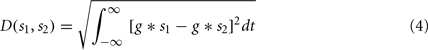
where g = g(t; τ_c) is a smoothing function (e.g., a decaying exponential) with time constant τ_c. Depending on the time constant τ_c, the distance metric interpolates between a coincidence detector (small time constant) and a rate difference counter (large time constant). Given the decay rate set for the synaptic update rule (see Sec. 2.4) we fixed τ_c = 4 ms, so that VRD is small for correlations that should trigger long term potentiation.

3. Results

We carried out experiments to demonstrate the emergence of feature sensitivity in the spiking neural network. We characterized the synaptic connectivity after exposure to ES and compared it to the predicted connectivity. We then measured the response of this network by probing with a set of PS that consisted of linear or forked frequency sweeps as shown in Figure 5 with different velocities; these results were used to determine the response curve after exposure. This was done first for the network with linearly distributed delay profile (see Figure 4), and subsequently with random delays.

FIGURE 4

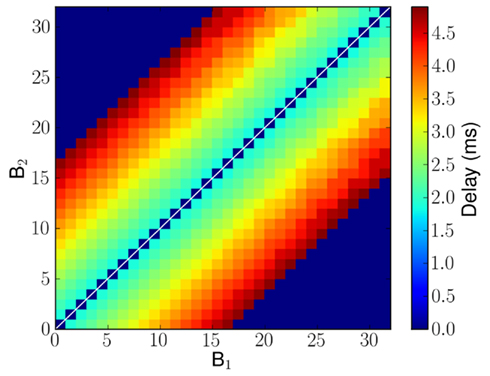
Figure 4. Implemented delayed projections from B₁ to B₂ neurons in millisecond. In case of no connection, it is marked as having 0 ms delay and is shown in blue. The delays were chosen from the ones available in the hardware implementation and so minor deviations from a pure linear profile can be observed.

FIGURE 5

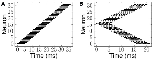
Figure 5. Spike patterns representing the two stimulus classes, linear and forked. Each dot represents a spike and the rate of sweep, the velocity, is given as the number of channels activated per millisecond. (A) Linear frequency sweep at 1.0 ms⁻¹. (B) Forked frequency sweep where the upper component is 1.0 ms⁻¹.

3.1. Distance Matrix and Emergent Connectivity

We define the distance matrix DM(i, j) as D(s_A(i), s_C(i, j)) between the spikes of neuron A in column i, that is, s_A(i), and the spikes of the neuron in population C of column i that was stimulated by the corresponding neuron B₁ in column j, that is, s_C(i, j) (see Figure 1).

Since spikes produced by the A neurons are the ones that drive the membrane potential of the B₂ neurons, the distance matrix DM(i, j) is tightly linked to the synaptic weight matrix of the B₁ to B₂ projections. Specifically, small VRD measures imply high probability of long term potentiation in the corresponding synapse.

Linear frequency sweeps at velocity of 5 ms⁻¹ were presented to the network as ES. Figure 6A shows the corresponding distance matrix DM(i, j). In case of no physical connection between i and j, we plot the distance D(s_A(i), s_NULL), where s_NULL is an empty spike train. This can be considered as a reference distance. Smaller values would represent more similar spike trains, and greater values more dissimilar ones. Figure 6B shows the potentiated synapses after stimulus presentation. As can be seen from the plots, the blue region in the distance matrix overlaps with the plot showing potentiated synapses. A similar comparison is made in Figure 8. Therefore this measure enables us to estimate the resulting connectivity after exposure.

FIGURE 6

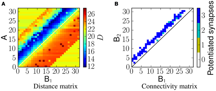
Figure 6. (A) The distance, D, between spikes produced by neurons in population A and spikes arriving at neurons in population B₂ for a network exposed to a linear frequency sweep at velocity of 1.0 ms⁻¹. (B) Corresponding synaptic weight matrix showing the number of potentiated synapses per projection from B₁ to B₂ neurons.

While the distance, D, acts as a coincidence measure between two spike trains, a time offset Δt in one of the spike trains enables us to measure their temporal correlation at a time offset τ between the two. By taking this measure of correlation across a range of values of Δt, one can effectively determine an optimal offset time τ that corresponds to maximal correlation between the two spike trains.

In the network described in section 2.1, the delayed projections do the job of implementing the time offset Δt and the plastic synapses potentiate only if these correlations are above a certain threshold.

Figure 7 shows the potentiated synapses after exposing the network to three different velocities of frequency sweeps. For a negative frequency sweep (decreasing frequency with time) the synapses below the diagonal are potentiated (Figure 7A) and above the diagonal otherwise (Figures 7B,C). For 1.2 ms⁻¹ frequency sweep the mean distance of potentiated synapses from the diagonal is greater than that for 0.8 ms⁻¹ frequency sweep.

FIGURE 7

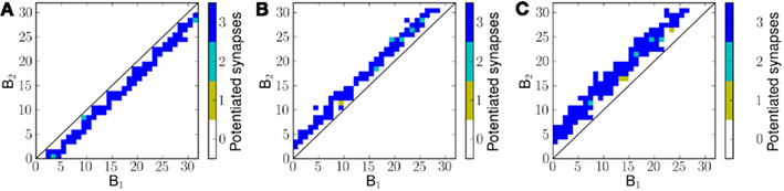
Figure 7. Potentiated synapses, or the effective final connectivity from B₁ neurons to B₂ neurons, after exposing the network to linear frequency sweeps at velocities (A) −0.8 ms⁻¹ (B) 0.8 ms⁻¹ and (C) 1.2 ms⁻¹.

It can be noted that the distance of potentiated synapses from the diagonal is determined by the velocity of the presented frequency sweep. This is because for a given velocity of frequency sweep, the optimal time offset Δt for maximal correlation between s_A(i) and s_C(i, j) is different; only those synapses for which the transmission delay Δt causes maximal correlation between s_A(i) and s_C(i, j) potentiate on exposure to a given stimulus.

Therefore the distance matrix DM is effectively a measure of temporal correlations in the stimulus. If some or all of the neurons in A were activated simultaneously (corresponding to ∞ ms⁻¹) the optimal time offset Δt for maximal correlation would be 0 ms or in other words this would enable the model to learn the purely spectral (or spatial) correlation in the input pattern. As the stimulus velocity decreases, the value of Δt for maximal correlation increases. Since the value of Δt between two neurons in the model depends on their distance of separation, we observe a corresponding change in the pattern of connectivity for different velocities of input stimulus.

When the network is exposed to a slightly more complex stimulus (the example we investigate is a forked frequency as shown in Figure 5B) the resulting connectivity is shown in Figure 8. It should be noted that the connectivity is not just a linear combination of upward frequency sweep and downward frequency sweep, but also captures the correlation between the two branches of sweeps, as predicted by the corresponding distance matrix shown in Figure 8A.

FIGURE 8

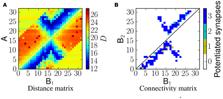
Figure 8. A comparison of the distance D to the potentiated synapses, for a network exposed to a forked frequency sweep at velocity 1.0 ms⁻¹. (A) VRD between the spike trains from A neurons and B₁ neurons that reach B₂ neurons. (B) Number of potentiated synapses per projection from B₁ to B₂ neurons.

All of the emergent connectivity matrices in these experiments emerged from exposure to the ES in an unsupervised manner. As shown by Figures 6 and 8 the post-exposure network connectivity always matches the area of minimum VRD in the distance matrix DM.

From this we can conclude that the network is capable of learning in a way determined by the spectro-temporal correlations in the stimulus. As the resulting connectivity closely matches the distance matrix DM, the potentiated synapses should support reliable network responses to stimuli with spectro-temporal features that closely match those of the ES. We verified this network property by measuring the Frequency Modulated (FM) sweep tuning curves, as described in the following section.

3.2. FM Sweep Tuning Curves

After exposing the network to 30 instances of the ES over a period of 3 s, we disabled synaptic plasticity while keeping all other network parameters unchanged. This is only necessary in this experiment because the learning rate of the network is set to be fast and presentation of any alternative stimulus would alter the synaptic states rather quickly. In these conditions we measured the response of the network, i.e., the total number of spikes from B₂ neurons, for different velocities of frequency sweeps. In the simplest case, linear sweeps of different velocities are used to measure the FM sweep tuning curve after training to a linear frequency sweep. In a second set of experiments forked sweeps of different velocities are used to measure the FM sweep tuning curve after training to a forked frequency sweep. These measurements were used to plot a tuning curve for the network. Figure 9 shows two tuning curves after learning a linear and forked frequency sweeps at 1.0 ms⁻¹. The tuning curves show a Gaussian-like profile which peaks at the velocity of ES. The width of the Gaussian is determined by the level of learning threshold þ, which is equivalent to the maximum D(s₁, s₂) below which the plastic synapses are set to potentiate and depress otherwise. This width of the tuning curve can be interpreted as the network’s resilience to variations in the time course of the stimulus.

FIGURE 9

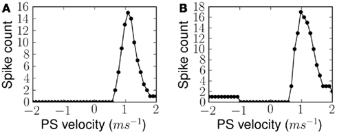
Figure 9. Measured FM sweep tuning curves after exposure to (A) linear and (B) forked stimulus, for ES velocity 1.0 ms⁻¹ in both cases. Response of the network is quantified by the number of output spikes from the population of B₂ neurons.

Qualitatively similar FM sweep tuning curves were obtained at different ES velocities for both linear and forked stimuli. This is shown in Figures 10A,B respectively. As can be noted the figures display maximal response along their diagonals implying maximum response to ES and lower response to any other.

FIGURE 10

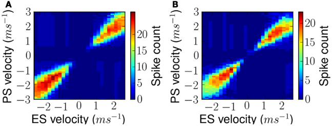
Figure 10. Measured FM sweep tuning curves after exposure as shown in Figure 9 but for all exposure stimuli. (A) Results for simple linear FM stimuli and (B) results for forked stimuli.

3.3. Random Delay Profile

The results described in the previous section were obtained with a linear delay profile as shown in Figure 3, i.e., the feedback delay was proportional to the distance between the B₁ and B₂ neurons.

But these conditions are not essential for the network to learn the spectro-temporal features of the ES and selectively respond to them. When the network is initialized with a random delay distribution, as shown in Figure 11A, learning potentiates the connections that represent the spectro-temporal correlation in the ES as described in the previous section. As long as the transmission delays Δt keep the corresponding distances D(s_A(i), s_C(i, j)) low, the corresponding synapses potentiate and learn to replicate the distance matrix DM(i, j).

FIGURE 11

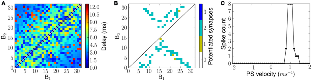
Figure 11. Connectivity and FM sweep tuning curve of a network with random transmission delays from B₁ neurons to B₂ neurons. (A) Transmission delays from B₁ neurons to B₂ neurons. (B) The number of potentiated synapses per projection from a B₁ neuron to B₂ neuron after exposure to forked frequency sweeps of velocity 1.0 ms⁻¹. (C) The measured tuning curve of the network after training.

The resulting network exhibits tuning properties similar to those observed for a linear delay profile. The connectivity matrix, after being exposed to forked frequency sweeps at 1.0 ms⁻¹ velocity is shown in Figure 11B and the sweep tuning curve of this network is shown in Figure 11C. Note that the tuning curves in Figures 9B and 11C show a similar performance although the network has a lower response level with random delay profile, which is explained by the fact that in the randomly connected examples only two, not three, synapses were available per B₂ neuron.

4. Conclusion

The results presented in this work demonstrate, in hardware, how an implementation of a recurrently connected spiking network is able to learn and selectively respond to the dynamic spectro-temporal features of stimuli. The model relies on delays, which might arise from a number of processes including axonal propagation and spike interaction via intermediate neurons.

In the case of the hardware substrate used to implement the model there was no provision for the implementation of delays in the design. We were able to overcome this problem by exploiting the variation and mismatch of the components in analog VLSI devices used in the setup.

The stimulus-driven modifications of the network connectivity result from the interaction between the stimulus itself and the spike-based plasticity (STDP) rule adopted for the delayed feedback connections. After learning, the firing patterns of the neurons reflect the emergent connectivity, that is more of the neurons fire during a presentation, and the network is tuned to the stimulus properties.

As a result, differences in the response of the network induced by learning can be used to distinguish similar stimuli that have parametrically different dynamic properties, for example differences in the direction or speed of an FM sweep.

Our experiments show, in spiking hardware and in a sensory context, the emergence of feature sensitivity, and the limitations imposed by demonstrating these effects in hardware have necessitated the choice of relatively simple stimulus patterns. However comparable results have also shown that the principles generalize to slightly more complex stimuli (Figure 5B) and, in software modeling work using a similar architecture, to dynamic ripples (Coath et al., 2011).

We have also demonstrated how the network with a random profile of transmission delays can exhibit similar behavior. This is important because random delay profiles imply that there is no structural necessity for the input neurons to be strictly tonotopically arranged. Therefore, without loss of generality, the input stimulus need not necessarily look well arranged as in Figure 5 and could be shuffled to appear as random patterns. By the same argument the network could also learn correlations in stimuli that are not so clearly ordered.

4.1. Exploiting Device Mismatch for Implementing Temporal Delays

In order to implement propagation delays we made use of extra neurons whose time constants were proportional to the desired time delay. We were able to select delay neurons with different time constants by exploiting the mismatch effect in their analog circuit implementations. The effect of this mismatch is shown in Figure 3, where we plot the range of delays exhibited by the neurons. Had there been no mismatch, this would not have been possible to achieve on a single chip with global/shared bias voltages. Variability can also be found on other model parameters (e.g., time constants, injection currents). This opens up the possibility to explore network dynamics of populations with a distribution of parameter values, rather than using globally common values. While mismatch induced noise is often minimized in conventional analog VLSI design, we try to use it to introduce sources of variability in the populations of silicon neurons that can model or reproduce the inhomogeneities present in real neural systems.

4.2. Long vs Short Time Scales

Sensory stimuli, and in particular auditory stimuli, contain both short and long range temporal correlations. The techniques described in this paper primarily address correlations only over relatively short time scales, i.e., those in a range from the order of synaptic or membrane time constants, up to those represented by the propagation of excitation to adjacent regions. The range of propagation delays implemented in the network defines the range of stimulus velocities that could be learnt. Temporal correlations over a longer time scale could be addressed using many levels of recurrence between widely separated layers, as is observed in the mammalian auditory system. Alternatively it could be tackled with working memory and neuromorphic implementations of state machine based approaches (Neftci et al., 2010).

4.3. Limitations

The network model described in the paper, in its current form, assumes the stimulus to be dynamic and does not consider static stimuli where frequency channels are persistently active. The learning rule used dictates high probability of LTP in the presence of highly active inputs. As a result, if such persistent stimuli were to be presented to this network a large number of synapses would potentiate to reflect the temporal correlation across different Δt values.

However transient responses, in particular onset responses, are found at all levels of the auditory system and this could be modeled with strong synaptic depression at the input synapses of B₁ and B₂ or as post-synaptic adaptation of neurons in A, thus eliminating the problems caused by persistent input stimuli.

5. Discussion

It is widely believed to be central to the performance of sensory systems in vivo that they respond preferentially to those aspects of the environment in which they operate that are salient. A simple biological example would be to differentiate a conspecific vocalization from the background of noise and other non-salient communication calls. Results suggest that this type of pattern specificity is, at least in some cases, present in primary cortical areas, e.g., Machens et al. (2004).

This same property is also an important goal of artificial sensory systems. In both cases this clearly requires some strategy for encoding salient features of the stimulus within the neural, or silicon substrate.

We propose that recurrent connectivity, observed throughout the auditory system, could mediate dynamic feature sensitivity by exploiting propagation delays. We have developed a computational model and verified that the emergent properties arise through the interaction of propagation delays with the spectro-temporal properties of stimuli and spike-time dependent plasticity.

While the representation of input stimuli in this network is realized through the pairing of activity at different times and at different positions on the tonotopic axis, it is not limited to a single pair. Each neuron in B₂, after learning, is connected to more than one B₁ neuron (see Figures 7 and 8B) in most cases. This leads to the B₂ neurons accumulating evidence from the spikes arriving from more than one B₁ neuron. If only a small fraction of the correlations present in the stimulus match those that have been learnt by the network, and if the threshold of the B₂ neurons was appropriately tuned (the threshold being the minimum number of coincident feedback spikes from B₁ for B₂ neurons to fire), then these neurons would not fire.

Consequently, we argue that given a large population and dense connectivity, a reasonable number of learned correlations from ES can be set as a threshold for the B₂ neurons to fire. The higher the number of such pairings present in a PS, the higher probability there is of the stimulus being identified as the current one (i.e., as ES).

The feature sensitivity represented in the model is not a property revealed in the firing rate of an individual neuron, or indeed in any property of an individual neuron. The model has widespread recurrent connections and as a consequence, the ensemble response of the network is modified during exposure. Thus the representation of, and sensitivity to, patterns of activity evolving over time is a network property of this model. This is especially interesting because clear examples of such dynamic response properties are routinely absent for single neuron measurements in vivo.

The neuromorphic system we describe here could be used with real-world stimuli and validated against noise in the stimulus, and limitations in the system’s state variables (e.g., due to device mismatch, limited resolution, and signal-to-noise ratio limitations, bounded synaptic weights, power constraints, etc.).

In further work, we plan to go beyond the demonstration of emergent sensitivity to a stimulus parameter, by quantifying the increase in acuity in information-theoretic terms in the presence of stimulus variation. This will provide a basis for the quantitative comparison of networks, connectivity patterns, and learning strategies.

Conflict of Interest Statement

The authors declare that the research was conducted in the absence of any commercial or financial relationships that could be construed as a potential conflict of interest.

Acknowledgments

This work was supported by the European Community’s Seventh Framework Programme (grants no. 231168-SCANDLE and no. 257219-neuroP), and by the Cluster of Excellence 277 (CITEC, Bielefeld University). We would like to thank our colleague Robert Mill for many helpful contributions made during the preparation of the manuscript. We would also like to thank Fabio Stefanini for helping with the hardware configuration and the NCS group (http://ncs.ethz.ch/) for contributing to the development of the AER and multi-chip experimental setup.

Footnotes

1. ^http://ine-web.org/workshops/workshops-overview
2. ^http://cne.ini.uzh.ch/capocaccia08/
3. ^As we are addressing auditory stimuli where the spatial dimension is tonotopic we use the term “spectro-temporal” throughout. This is equivalent to “spatio-temporal” in other modalities.

References

Abdalla, H., and Horiuchi, T. K. (2008). “Spike-based acoustic signal processing chips for detection and localization,” in Biomedical Circuits and Systems Conference, BIOCAS 2008, IEEE, Baltimore, 225–228.

Atencio, C. A., Blake, D. T., Strata, F., Cheung, S. W., Merzenich, M. M., and Schreiner, C. E. (2007). Frequency-modulation encoding in the primary auditory cortex of the awake owl monkey. J. Neurophysiol. 98, 2182–219.

Pubmed Abstract | Pubmed Full Text | CrossRef Full Text

Atencio, C. A., and Schreiner, C. E. (2010). Laminar diversity of dynamic sound processing in cat primary auditory cortex. J. Neurophysiol. 103, 192–205.

Pubmed Abstract | Pubmed Full Text | CrossRef Full Text

Barbaro, M., Burgi, P.-Y., Mortara, A., Nussbaum, P., and Heitger, F. (2002). A 100x100 pixel silicon retina for gradient extraction with steering filter capabilities and temporal output coding. IEEE J. Solid-State Circuits 37, 160–172.

CrossRef Full Text

Bartolozzi, C., and Indiveri, G. (2007). Synaptic dynamics in analog VLSI. Neural Comput. 19, 2581–2603.

Pubmed Abstract | Pubmed Full Text | CrossRef Full Text

Boahen, K. A. (2000). Point-to-point connectivity between neuromorphic chips using address-events. IEEE Trans. Circuits Syst. 47, 416–434.

CrossRef Full Text

Brader, J. M., Senn, W., and Fusi, S. (2007). Learning real-world stimuli in a neural network with spike-driven synaptic dynamics. Neural Comput. 19, 2881–2912.

Pubmed Abstract | Pubmed Full Text | CrossRef Full Text

Calhoun, B. M., and Schreiner, C. E. (1998). Spectral envelope coding in cat primary auditory cortex: linear and non-linear effects of stimulus characteristics. Eur. J. Neurosci. 10, 926–940.

Pubmed Abstract | Pubmed Full Text | CrossRef Full Text

Caporale, N., and Dan, Y. (2008). Spike timing dependent plasticity: a Hebbian learning rule. Annu. Rev. Neurosci. 31, 25–46.

Pubmed Abstract | Pubmed Full Text | CrossRef Full Text

Chan, V., Liu, S.-C., and van Schaik, A. (2007). AER EAR: a matched silicon cochlea pair with address event representation interface. IEEE Trans. Circuits Syst. I Regul. Pap. 54, 48–59.

CrossRef Full Text

Chicca, E., Whatley, A. M., Lichtsteiner, P., Dante, V., Delbruck, T., Del Giudice, P., Douglas, R. J., and Indiveri, G. (2007). A multi-chip pulse-based neuromorphic infrastructure and its application to a model of orientation selectivity. IEEE Trans. Circuits Syst. I Regul. Pap. 5, 981–993.

CrossRef Full Text

Choi, T. Y. W., Merolla, P. A., Arthur, J. V., Boahen, K. A., and Shi, B. E. (2005). Neuromorphic implementation of orientation hypercolumns. IEEE Trans. Circuits Syst. I Regul. Pap. 52, 1049–1060.

CrossRef Full Text

Coath, M., Mill, R., Denham, S. L., and Wennekers, T. (2011). Emergent Feature Sensitivity in a Model of the Auditory Thalamocortical System, Volume 718 of Advances in Experimental Medicine and Biology. New York: Springer, 7–17.

Culurciello, E., Etienne-Cummings, R., and Boahen, K. (2003). A biomorphic digital image sensor. IEEE J. Solid-State Circuits 38, 281–294.

CrossRef Full Text

Davison, A. P., Brüderle, D., Eppler, J., Kremkow, J., Muller, E., Pecevski, D., Perrinet, L., and Yger, P. (2008). PyNN: a common interface for neuronal network simulators. Front. Neuroinform. 2:11. doi:10.3389/neuro.11.011.2008

CrossRef Full Text

Deiss, S. R., Douglas, R. J., and Whatley, A. M. (1999). “A pulse-coded communications infrastructure for neuromorphic systems,” in Pulsed Neural Networks, Chap. 6, eds W. Maass and C. M. Bishop (Cambridge: MIT Press), 157–178.

Depireux, D. A., Simon, J. Z., Klein, D. J., and Shamma, S. A. (2001). Spectro-temporal response field characterization with dynamic ripples in ferret primary auditory cortex. J. Neurophysiol. 85, 1220–1234.

Pubmed Abstract | Pubmed Full Text

Fasnacht, D. B., and Indiveri, G. (2011). “A PCI based high-fanout AER mapper with 2 GiB RAM look-up table, 0.8 (s latency and 66 MHz output event-rate,” in Conference on Information Sciences and Systems, CISS 2011, Baltimore: Johns Hopkins University, 1–6.

Fasnacht, D. B., Whatley, A. M., and Indiveri, G. (2008). “A serial communication infrastructure for multi-chip address event system,” in International Symposium on Circuits and Systems, ISCAS 2008, IEEE, Seattle, 648–651.

Folowosele, F., Vogelstein, R. J., and Etienne-Cummings, R. (2008). “Real-time silicon implementation of V1 in hierarchical visual information processing,” in Biomedical Circuits and Systems Conference, BIOCAS 2008, IEEE, Baltimore, 181–184.

Fragnière, E., van Schaik, A., and Vittoz, E. (1997). Design of an analogue VLSI model of an active cochlea. J. Analog Integr. Circuits Signal Process. 13, 19–35.

CrossRef Full Text

Fusi, S. (2003). Spike-driven synaptic plasticity for learning correlated patterns of mean firing rates. Rev. Neurosci. 14, 73–84.

Pubmed Abstract | Pubmed Full Text | CrossRef Full Text

Giulioni, M., Pannunzi, M., Badoni, D., Dante, V., and Del Giudice, P. (2009). Classification of correlated patterns with a configurable analog VLSI neural network of spiking neurons and self-regulating plastic synapses. Neural Comput. 21, 3106–3129.

Pubmed Abstract | Pubmed Full Text | CrossRef Full Text

Godey, B., Atencio, C. A., Bonham, B. H., Schreiner, C. E., and Cheung, S. W. (2005). Functional organization of squirrel monkey primary auditory cortex: responses to frequency-modulation sweeps. J. Neurophysiol. 94, 1299–1311.

Pubmed Abstract | Pubmed Full Text | CrossRef Full Text

Gomez-Rodriguez, F., Paz, R., Linares-Barranco, A., Rivas, M., Miro, L., Vicente, S., Jimenez, G., and Civit, A. (2006). “AER tools for communications and debugging,” in International Symposium on Circuits and Systems, ISCAS 2006, IEEE, Island of Kos, 3253–3256.

Hofstaetter, M., Schoen, P., and Posch, C. (2010). “A SPARC-compatible general purpose address-event processor with 20-bit 10ns-resolution asynchronous sensor data interface in 0.18(m CMOS,” in International Symposium on Circuits and Systems, ISCAS 2010, IEEE, Paris, 4229–4232.

Indiveri, G., Chicca, E., and Douglas, R. J. (2006). A VLSI array of low-power spiking neurons and bistable synapses with spike-timing dependent plasticity. IEEE Trans. Neural Netw. 17, 211–221.

Pubmed Abstract | Pubmed Full Text | CrossRef Full Text

Indiveri, G., and Horiuchi, T. K. (2011). Frontiers in neuromorphic engineering. Front. Neurosci. 5:118. doi:10.3389/fnins.2011.00118

CrossRef Full Text

Indiveri, G., Linares-Barranco, B., Hamilton, T. J., van Schaik, A., Etienne-Cummings, R., Delbruck, T., Liu, S.-C., Dudek, P., Häfliger, P., Renaud, S., Schemmel, J., Cauwenberghs, G., Arthur, J., Hynna, K., Folowosele, F., Saighi, S., Serrano-Gotarredona, T., Wijekoon, J., Wang, Y., and Boahen, K. (2011). Neuromorphic silicon neuron circuits. Front. Neurosci. 5:73. doi:10.3389/fnins.2011.00073

CrossRef Full Text

Jin, X., Lujan, M., Plana, L. A., Davies, S., Temple, S., and Furber, S. (2010). Modeling spiking neural networks on SpiNNaker. Comput. Sci. Eng. 12, 91–97.

CrossRef Full Text

Koch, C., and Mathur, B. (1996). Neuromorphic vision chips. IEEE Spectr. 33, 38–46.

CrossRef Full Text

Kowalski, N., Depireux, D. A., and Shamma, S. A. (1996). Analysis of dynamic spectra in ferret primary auditory cortex. II. Prediction of unit responses to arbitrary dynamic spectra. J. Neurophysiol. 76, 3524–3534.

Pubmed Abstract | Pubmed Full Text

Kramer, J. (2002). “An ON/OFF transient imager with event-driven, asynchronous readout,” in International Symposium on Circuits and Systems, ISCAS 2002, IEEE, Scottsdale.

Leñero-Bardallo, J. A., Serrano-Gotarredona, T., and Linares-Barranco, B. (2010). A five-decade dynamic-range ambient-light-independent calibrated signed-spatial-contrast AER retina with 0.1-ms latency and optional time-to-first-spike mode. IEEE Trans. Circuits Syst. I Regul. Pap. 57, 2632–2643.

CrossRef Full Text

Lichtsteiner, P., Posch, C., and Delbruck, T. (2006). “A 128 (128 120dB 30mW asynchronous vision sensor that responds to relative intensity change,” in IEEE ISSCC Digest of Technical Papers, IEEE, San Francisco, 508–509.

Liu, S.-C. (1999). Silicon retina with adaptive filtering properties. J. Analog Integr. Circuits Signal Process. 18, 243–254.

CrossRef Full Text

Liu, S.-C., Kramer, J., Indiveri, G., Delbruck, T., Burg, T., and Douglas, R. J. (2001). Orientation-selective aVLSI spiking neurons. Neural Netw. 14, 629–643.

Pubmed Abstract | Pubmed Full Text | CrossRef Full Text

Machens, C. K., Wehr, M. S., and Zador, A. M. (2004). Linearity of cortical receptive fields measured with natural sounds. J. Neurosci. 24, 1089.

Pubmed Abstract | Pubmed Full Text | CrossRef Full Text

Mitra, S., Fusi, S., and Indiveri, G. (2009). Real-time classification of complex patterns using spike-based learning in neuromorphic VLSI. IEEE Trans. Biomed. Circuits Syst. 3, 32–42.

CrossRef Full Text

Neftci, E., Chicca, E., Cook, M., Indiveri, G., and Douglas, R. J. (2010). “State-dependent sensory processing in networks of VLSI spiking neurons,” in International Symposium on Circuits and Systems, ISCAS 2010, IEEE, Paris, 2789–2792.

Neftci, E., Chicca, E., Indiveri, G., and Douglas, R. J. (2011). A systematic method for configuring VLSI networks of spiking neurons. Neural Comput. 23, 2457–2497.

Pubmed Abstract | Pubmed Full Text | CrossRef Full Text

Neftci, E., and Indiveri, G. (2010). “A device mismatch compensation method for VLSI spiking neural networks,” in Biomedical Circuits and Systems Conference BIOCAS 2010, IEEE, Paphos, 262–265.

Neftci, E., Toth, B., Indiveri, G., and Abarbanel, H. (2012). Dynamic state and parameter estimation applied to neuromorphic systems. Neural Comput. (in press).

Scholze, S., Schiefer, S., Hartmann, J., Mayr, C., Höppner, S., Eisenreich, H., Henker, S., Vogginger, B., and Schüffny, R. (2011). VLSI implementation of a 2.8 Gevent/s packet based AER interface with routing and event sorting functionality. Front. Neurosci. 5:117. doi:10.3389/fnins.2011.00117

CrossRef Full Text

Serrano-Gotarredona, R., Oster, M., Lichtsteiner, P., Linares-Barranco, A., Paz-Vicente, R., Gómez-Rodríguez, F., Camunas-Mesa, L., Berner, R., Rivas-Perez, M., Delbruck, T., Liu, S.-C., Douglas, R., Häfliger, P., Jimenez-Moreno, G., Civit-Ballcels, A., Serrano-Gotarredona, T., Acosta-Jiménez, A. J., and Linares-Barranco, B. (2009). CAVIAR: a 45k neuron, 5M synapse, 12G connects/s AER hardware sensory-processing-learning-actuating system for high-speed visual object recognition and tracking. IEEE Trans. Neural Netw. 20, 1417–1438.

Pubmed Abstract | Pubmed Full Text | CrossRef Full Text

Sheik, S., Stefanini, F., Neftci, E., Chicca, E., and Indiveri, G. (2011). “Systematic configuration and automatic tuning of neuromorphic systems,” in International Symposium on Circuits and Systems, ISCAS 2011, IEEE, Rio de Janeiro, 873–876.

Shouval, H. Z., Bear, M. F., and Cooper, L. N. (2002). A unified model of NMDA receptor-dependent bidirectional synaptic plasticity. Proc. Natl. Acad. Sci. U.S.A. 99, 10831–10836.

Pubmed Abstract | Pubmed Full Text | CrossRef Full Text

Toumazou, C., Ngarmnil, J., and Lande, T. S. (1994). Micropower log-domain filter for electronic cochlea. Electron. Lett. 30, 1839–1841.

CrossRef Full Text

van Rossum, M. C. (2001). A novel spike distance. Neural Comput. 13, 751–763.

Pubmed Abstract | Pubmed Full Text | CrossRef Full Text

van Schaik, A., Fragnière, E., and Vittoz, E. (1996). “Improved silicon cochlea using compatible lateral bipolar transistors,” in Advances in Neural Information Processing Systems, Vol. 8, eds D. S. Touretzky, M. C. Mozer, and M. E. Hasselmo (Cambridge, MA: MIT Press), 671–677.

van Schaik, A., and Meddis, R. (1999). Analog very large-scale integrated (VLSI) implementation of a model of amplitude-modulation sensitivity in the auditory brainstem. J. Acoust. Soc. Am. 105, 811.

Pubmed Abstract | Pubmed Full Text | CrossRef Full Text

Watts, L., Kerns, D. A., Lyon, R. F., and Mead, C. A. (1992). Improved implementation of the silicon cochlea. IEEE J. Solid-State Circuits 27, 692–700.

CrossRef Full Text

Wen, B., and Boahen, K. (2006). “Active bidirectional coupling in a cochlear chip,” in Advances in Neural Information Processing Systems, Vol. 18, eds Y. Weiss, B. Schölkopf, and J. Platt (Cambridge, MA: MIT Press), 1497–1504.

Ye, C. Q., Poo, M. M., Dan, Y., and Zhang, X. H. (2010). Synaptic mechanisms of direction selectivity in primary auditory cortex. J. Neurosci. 30, 1861–1868.

Pubmed Abstract | Pubmed Full Text | CrossRef Full Text

Zaghloul, K. A., and Boahen, K. (2006). A silicon retina that reproduces signals in the optic nerve. J. Neural Eng. 3:257–267.

Pubmed Abstract | Pubmed Full Text | CrossRef Full Text