Neuromorphic Audio-Visual Sensor Fusion on a Sound-Localising Robot

This paper presents the first robotic system featuring audio–visual (AV) sensor fusion with neuromorphic sensors. We combine a pair of silicon cochleae and a silicon retina on a robotic platform to allow the robot to learn sound localization through self motion and visual feedback, using an adaptive ITD-based sound localization algorithm. After training, the robot can localize sound sources (white or pink noise) in a reverberant environment with an RMS error of 4–5° in azimuth. We also investigate the AV source binding problem and an experiment is conducted to test the effectiveness of matching an audio event with a corresponding visual event based on their onset time. Despite the simplicity of this method and a large number of false visual events in the background, a correct match can be made 75% of the time during the experiment.

Introduction

Neuromorphic engineering, introduced by Carver Mead in the late 1980s, is a multidisciplinary approach to artificial intelligence, building bio-inspired sensory and processing systems by combining neuroscience, signal processing, and analog VLSI (Mead, 1989; Mead, 1990). Learning from biology and observing the principles employed, neuromorphic engineers seek to replicate many of the sensory–motor tasks that biology excels at and seemingly performs with ease.

Neuromorphic engineering follows several design paradigms taken from biology and these are: (1) pre-processing at the sensor front-end to increase dynamic range; (2) adaptation over time to learn and minimize systematic errors; (3) efficient use of transistors for low precision computation; (4) parallel processing; and (5) signal representation by discrete events (spikes) for efficient and robust communication. Further, by-products of implementation in analog VLSI include low power consumption and real time operation.

Although there are many examples of neuromorphic sensors being incorporated into sensory systems and robots, to date, however, most neuromorphic systems are limited to the use of only one type of sensor (Gomez-Rodriguez et al., 2007; Linares-Barranco et al., 2007; Jimenez-Fernandez et al., 2008). Systems that combine multiple sensors exist but the sensors are still restricted to one modality, for example, vision (Becanovic et al., 2004). While audio–visual (AV) sensor fusion has been studied for a long time in the field of robotics, with examples such as (Bothe et al., 1999; Wong et al., 2008), to our knowledge, there are no neuromorphic systems which combine sensors of different modalities.

By combining different sensory modalities, a sensory system can operate in a wider range of environments by taking advantage of the different senses. This applies to both traditional and neuromorphic systems alike. In situations when one sense is absent, the system can continue to operate by relying on the other senses. On the other hand, in situations when multiple senses are available, accuracy can be improved by combining the information from the different senses. In addition, it is possible to derive information not obtainable from one sense alone. A good example would be to determine the distance of an AV source based on the difference in arrival times of light and sound due to their difference in speed. An additional benefit of studying sensor fusion in the context of neuromorphic engineering is that it allows us to test the principles learnt from biology and gives us better insights into how fusion is performed by the brain.

In this paper, we combine a pair of silicon cochleae and a silicon retina in a neuromorphic system to allow a robot to learn to localize audio and visual sources, as a first step toward multi-modal neuromorphic sensor fusion. The cochlea chip contains a matched pair of silicon cochleae with 32 channels each and outputs spikes using the address-event protocol, while the retina chip is a 40-by-40 pixels vision sensor capable of detecting multiple onset events and it also uses the address-event protocol to communicate the positions of these events. Source localization is an important area to start with because the detection of an object in the surrounding environment is prerequisite to interacting with it, whether it is a person, an animal, a vehicle, or another robot.

In a previous paper in this journal, we introduced and tested an adaptive ITD-based¹ sound localization algorithm that employs a pair of silicon cochleae, the AER EAR, and supports online learning (Chan et al., 2010). We continue the work here by combining the sound localization system with a transient vision sensor (Chan et al., 2007a) to develop a neuromorphic AV source localization system on a robotic platform. In a first experiment, we investigate the possibility of using self motion and visual feedback to train a robot to accurately localize a sound source in a reverberant environment and turn toward it. In a second experiment, we look at the binding problem in the event of multiple visual sources. We test the effectiveness of matching an audio source with the corresponding visual source by comparing their onsets. In Section “Materials and Methods,” we will introduce our methods including the robotic platform, the experimental setup and the training procedure. The results will be presented in Section “Results,” while Section “Conclusion” will discuss the results and conclude the paper.

Materials and Methods

Robotic Platform

We chose the Koala robot made by K-Team (2008) as our robotic platform. Being a medium-size robot, measuring about 30 cm in length and width, it provided sufficient space for the mounting of the sensors and the circuit boards. It was driven by six wheels with three on each side and the wheels on either side could be controlled independently. This allowed the robot to rotate on the spot by driving the wheels in opposite directions. The position of each wheel was monitored by an onboard controller to precisely control the robot’s movement. Since the only movement required in the experiments described here was rotation, the robot was tied to an anchor point on the floor to prevent it from drifting throughout the course of the experiment.

A pair of microphones were mounted on opposite sides of a foam sphere (15 cm in diameter), with the sphere itself fixed atop the Koala (Figures 1A,B). The microphone signals were amplified and fed into the cochlea board located beneath the sphere. The silicon cochlea chip with AER interface has been described in detail in (van Schaik and Liu, 2005; Chan et al., 2007b), and was setup almost exactly the same as described in (Chan et al., 2010). The cochlea channels were tuned to cover the frequency range from 200- to 10-kHz logarithmically, and each channel generated, on average, 6000 spikes/s when the stimulus was played from a loudspeaker. The higher frequency channels (>3 kHz) were not used for localization because ITD is ambiguous at those frequencies. The only difference in the auditory setup from (Chan et al., 2010) was the lack of simulated automatic gain control because the stimuli were no longer synthesized on a PC and fed to the cochleae directly, as was the case in (Chan et al., 2010).

FIGURE 1

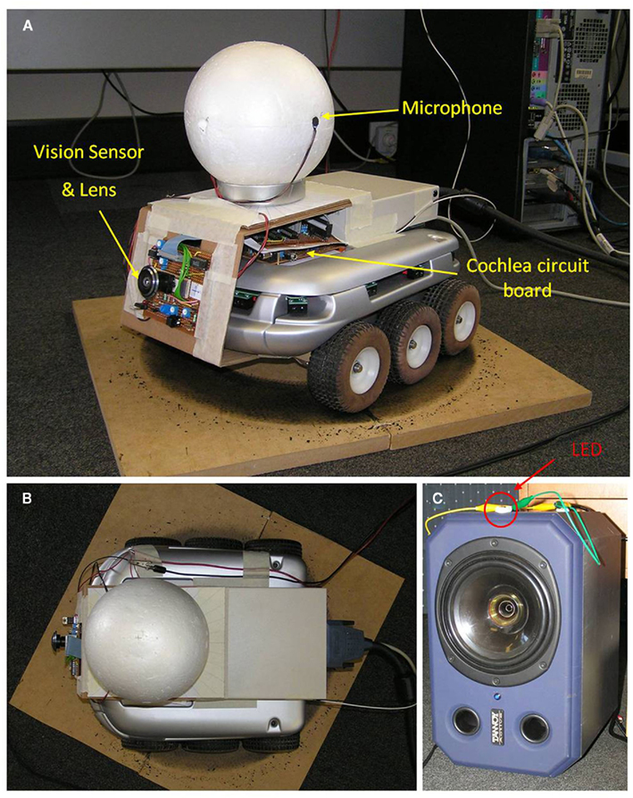
Figure 1. (A)The Koala robot with the foam sphere mounted on top to emulate a head. The signals received by a pair of microphones, mounted on opposite sides of the sphere, were fed to the cochlea board located beneath the sphere. The vision sensor fitted with an ultra-wide angle lens was mounted at the front of the robot. The AER outputs from the cochlea and the vision sensor were then combined and collected by a PCI DAQ card via the cable at the back of the robot. (B) Top view of the robot. (C) The AV source consisting of a loudspeaker with a flashing LED at the top. The LED allowed the robot to locate the source using the vision sensor.

The transient vision sensor (Chan et al., 2007a) was fit to the front of the Koala with an ultra-wide angle lens providing a fish-eye view (Figure 1A). The lens itself could provide 180° field of view (FOV) but the actual FOV was limited to 50° by the relatively small size of our sensor array (1.8 mm × 1.8 mm). Nevertheless, this FOV was sufficient for our experiment. The vision sensor contained 40 × 40 pixels and returned the x–y coordinates of detected transient events.

Both the AER EAR and the transient sensor used the multi-sender AER protocol (Deiss, 1994; Deiss et al., 1998) for communication, allowing their outputs to be merged onto a common bus by an external arbiter circuit built from logic gates and latches. These events were then collected by a PCI digital data acquisition (DAQ) card on a PC. All subsequent processing was performed in MATLAB. This PC also controlled the robot’s movement via a serial connection.

Acoustic Environment and Audio–Visual Stimulus

The experiments were conducted in an office environment. The stimuli were played in the presence of background noises generated by computers, air-conditioning, and human activities. There were also reverberations from the walls, the floor, and the surrounding furniture.

The audio stimulus used was pink noise with a spectrum from 200- to 3-kHz. Pink noise was chosen because of its 1/f power spectrum, providing equal amount of energy to the cochlea channels which were logarithmically spaced. This allowed the channels to contribute equally to the localization and enabled learning to take place at all frequency bands simultaneously. The stimulus was played from a loudspeaker (Tannoy System 600A), placed at a distance of 2.5 m from the robot. In all the experiments, the sound level of the stimulus is approximately 70 dB SPL measured at the robot. The Tannoy loudspeaker featured concentric bass driver and tweeter unit to provide a single point source for all audio frequencies, and had a flat spectrum from 44- to 20-kHz.

In our first experiment, an LED flashing at 35-Hz was mounted on the loudspeaker (Figure 1C) to allow the robot to locate it visually when it came into the FOV. This unique frequency was chosen to easily differentiate it from the other objects, including false detections caused by the fluorescence lighting, which flickers at 100-Hz.

Although this method of identifying the AV source was very reliable, it is impractical for most applications because it requires prior knowledge about the source. In situations where no such information is available, it is possible to extract the AV source from a number of visual objects in the background by assuming some correlations between the audio and visual stimuli. In the second experiment, we tested the effectiveness of binding the audio source with the corresponding visual source based on their onsets. There were three primary visual sources in the experiment, plus some objects in the background caused by the fluorescent lighting which flickered at 100-Hz. The first source was the LED flashing at 35-Hz, used in the first experiment to locate the speaker. The second source was an LED flashing at a lower frequency of 15-Hz, while the third source was a third LED which was in sync with the audio stimulus (Figure 2). All three LEDs were placed in front of the robot. The robot was only allowed to rotate within a small range so that the LEDs were always in its FOV. The objective was to identify the third LED from the other visual objects.

FIGURE 2

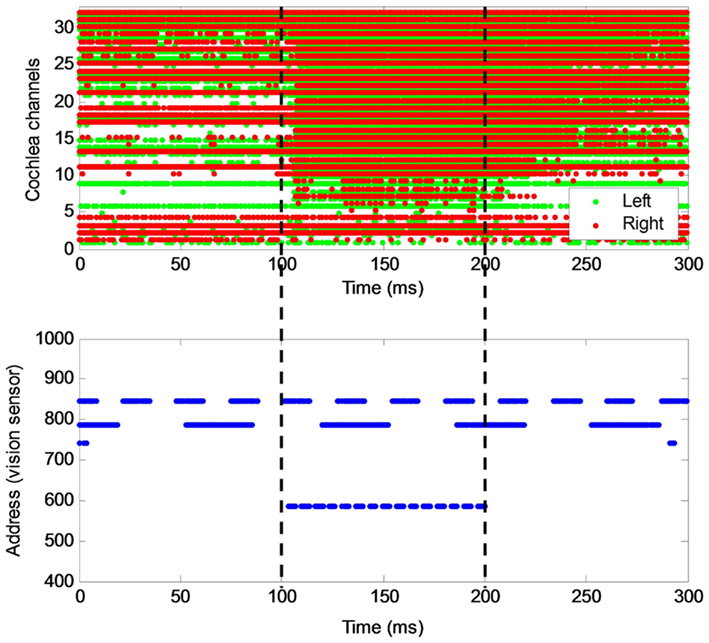
Figure 2. The AER outputs from the cochlea and the vision sensor, over a period of 300 ms. Many of the cochlea channels had a background firing rate. All cochlea channels generated spikes at a much higher rate as soon as the pink noise stimulus was played at 100 ms. At the vision sensor, three major light sources were shown. The first two were periodic with frequencies of 35- and 15-Hz. The third visual source was in sync with the audio stimulus. The vertical dotted lines indicate the start and end of the stimuli.

Sound Localization Learning Algorithm for Experiment 1

An adaptive ITD-based sound localization algorithm was previously proposed, which supports online learning, making it ideally suited for learning with feedback (Chan et al., 2010). A brief description is given here. Audio signals from the left and right microphones are first processed by the left and the right cochleae, which divide them into different frequency bands and convert the signals into spike trains. At each frequency band, after cross-correlation of the left and right spike trains and application of soft-WTA², the resulting vector, S, is multiplied by a weight matrix, W, to produce a vector G.

G represents auditory activity at different azimuths (−90° to 90° with 3° step) and is expected to be maximum at the position corresponding to the direction of the sound source. The resulting G’s from all the frequency bands are then summed and a WTA is used to produce a global estimate by selecting the azimuth with the highest overall activity. By adjusting the weight matrices, the system can adapt and learn to localize sound. The weight update rule is

where ε is the learning rate, S^T is the transpose of S, and T is the target auditory activity function, which is a Gaussian function centered at the target’s azimuth position with a SD of 25°. This target function was chosen because the Gaussian function is a natural spreading function and some initial testing indicates a 25° SD works well.

The Koala was trained to localize sound through iterations of sensing and motion, similar to the work published by Nakashima and Hornstein (Nakashima et al., 2002; Hornstein et al., 2006), with our neuromorphic sound localization algorithm incorporated. The procedure consisted of the following steps:

1. Turn the Koala to the frontal position with the source straight ahead, using the vision sensor to zero-in on the source.

2. Select a random azimuth, θ, from the range [−90°, 90°] with 10° step.

3. Turn the Koala by −θ, such that the source is now at θ azimuth relative to the robot.

4. Play pink noise stimulus and record the spikes from the AER cochlea simultaneously for 200 ms.

5. The spike trains are processed with the sound localization algorithm to produce an estimate, .

6. Turn the Koala to the estimated direction.

7. Use the vision sensor to locate the position of the source relative to the robot by identifying the flashing LED. This gives the localization error θ_e. True position of the source can then be determined from and the weight matrices are updated according to Eq. (2).

8. If the source is not in view (i.e., localization error > 25°), then no update will be performed on the weights³. However, the localization error can still be calculated from the source’s true position (θ) and its estimate (θ_e). This error is used only to monitor the progress in the Koala’s learning.

Steps 1–8 were repeated for each azimuth (19 positions in total) during each epoch. The average RMS error was calculated after each epoch.

Figure 3 shows a block diagram of the complete system. All processing after the AER EAR and the vision sensor was performed in MATLAB. In the visual processing stream, the “Identify Source” step identified the flashing LED in the event of multiple visual objects. It involved matching the spike train from each object with the predetermined frequency of our LED (35-Hz) and returning the address of the object of best match.

FIGURE 3

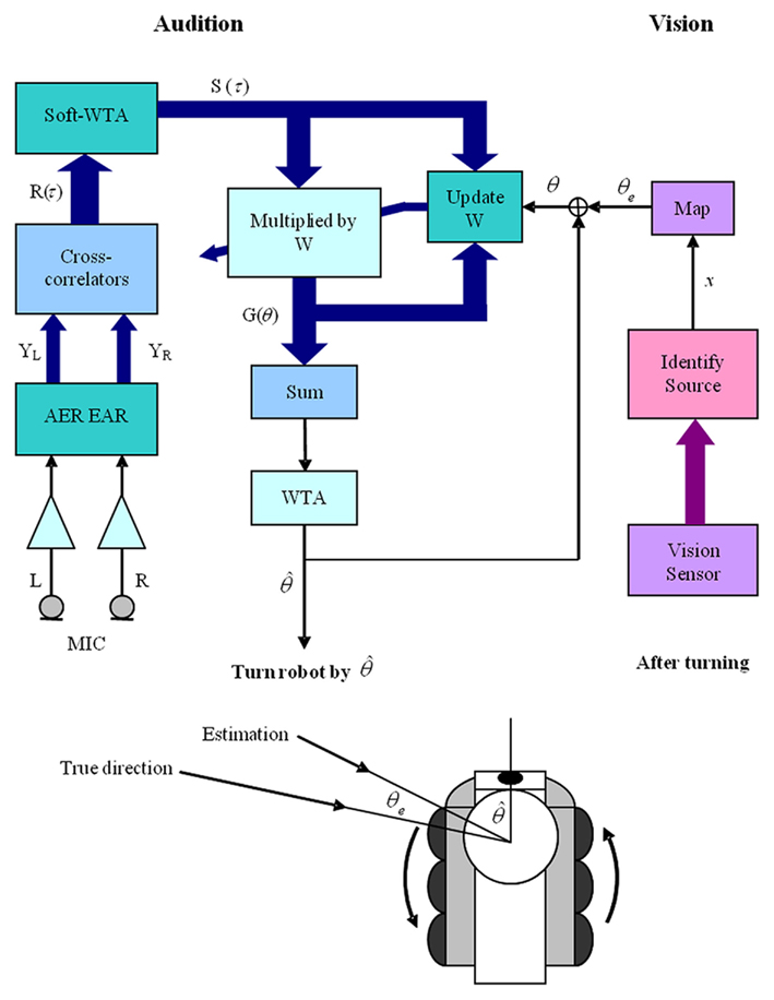
Figure 3. Block diagram of the complete audio–visual system. L and R were the audio signals from the microphones. Y_L and Y_R were the spikes generated by the AER EAR. R(τ) and S(τ) were the cross-correlation results and soft-WTA results, respectively. G(θ) is the product of S(τ) and the weight matrices W, and it represents the auditory activities. After a sound was presented, the robot would turn toward , the direction estimated by the localization algorithm. The true position of the source was then found by mapping the vision sensor output (x, y) to θ_e and updates could be made to W, during the learning process. The thick arrows in the auditory processing path indicate signals in multiple frequency bands. In the vision module, the thick arrow represents the multiple objects detected by the vision sensor.

Source Binding Algorithm for Experiment 2

Figure 4 shows the implementation of source binding based on the onset times. For simplicity, we assumed a single sound source. Therefore, the onset time of the sound could be determined by summing the spikes from all the channels and using an onset detector to look for a sudden increase in the overall spike rate. The onset detector consisted of a first-order low-pass filter (LPF), a differentiator and a comparator. The LPF removed fluctuation in spike rates to minimize false detection. The differentiator computed the rate of change and caused the comparator to go high if the rate of increase was above a threshold. For a step input, the onset detector would output a pulse, with the pulse width determined by the size of the step, the cut-off frequency of the LPF, and the threshold. For this experiment, we have set the cut-off frequency to 20-Hz. A low cut-off frequency was used because we were only interested in the envelope of the stimulus, not its fine temporal structure. It also resulted in a longer pulse at the output for more reliable operation. Figure 5 showed the onset detector picking up the onset from the outputs of the AER cochlea.

FIGURE 4

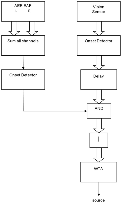
Figure 4. A block diagram of the source binding algorithm based on onset time. See text for details.

FIGURE 5

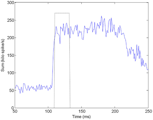
Figure 5. The figure shows the result of summing the spikes across all cochlea channels (solid line) and the output of the onset detector (dotted line). There was a small delay due to the LPF at the onset detector. The delay, however, would not affect the final result because the same delay was also present in the visual processing.

Onset detection was also applied to each visual object detected by the sensor. A delay was then added to account for the systematic delay introduced by the cochlea, as well as the delay due to the difference in arrival time of light and sound due to their difference in speed. This delay was a function of the source’s distance and is set to 10 ms in this experiment. Figure 6 showed the delayed onset detector outputs for several visual objects. There was a good match between the onset detected from the audio stimulus and that from the third LED.

FIGURE 6

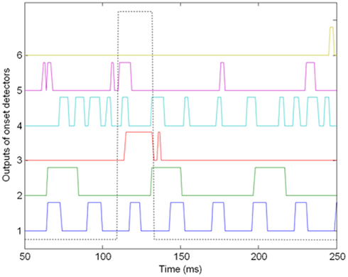
Figure 6. The delayed onset detector outputs for six visual objects detected by the vision sensor. Object 1 and 2 were the LEDs flashing at 35- and 15-Hz, respectively. Object 3 was the LED synchronized with the audio stimulus, which we were attempting to identify. Object 4–6 were simply background objects due to the fluorescent lighting. The onset detected from the audio stimulus was also shown in dotted line.

As shown in Figure 4, a logical AND operation was performed with the onset detector output from the audio stimulus and the delayed onset detector outputs from each of the visual objects, followed by an integration step, producing a value that was proportional to the amount of overlap between the onset detector output from the audio stimulus and those from the visual objects. The visual object with the best match in onset time would result in the largest overlap and would be selected by the winner-take-all. For simplicity, the entire source binding algorithm was implemented in software.

Calibration of Robot Movement and Vision Sensor

Turning of the Koala was accomplished by driving the wheels on either side in opposite directions. The relationship between the wheel position and the direction of the robot was linear, allowing us to easily control the turning. However, it was found that after repeated turning, the robot would slowly drift to one side due to wheel slipping. This drift was minimized during the experiment by returning the robot to the frontal position (0°) before the presentation of every stimulus. After calibration, turning was accurate to within 1–2° over the [−90°, 90°] range.

When the vision sensor detected a transient object, it returned an address of the form (x, y), which was a function of (θ, ϕ), the azimuth and elevation of the object relative to the robot. The exact relationship depended on the optics in the lens and any misalignment when the lens and the sensor were mounted on the robot. In our experiments, since the elevation was fixed, the mapping was simplified to þeta = f(x). This mapping was determined by recording the x addresses when the target was at different azimuths and fitting a third-order polynomial to the data. The azimuth of visual objects could be determined to within 1° over the entire FOV, with the accuracy primarily limited by the resolution of the sensor, which contained only 40 pixels horizontally.

Results

Experiment 1

We tested the Koala with the pink noise stimulus over the range of azimuth from −90° to 90°, with 5° steps. Initially, the weights had not been trained for our experimental setup and the robot systematically underestimated the direction of the source. The results over five trials are shown in Figure 7 and it can be seen that the localization results are poor. Due to length constraint, the intermediate results from the cross-correlator, soft-WTA and weight multiplication are not shown here, but examples of intermediate signals can be found in our previous paper (Chan et al., 2010).

FIGURE 7

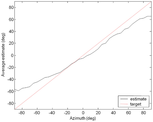
Figure 7. Initial localization results.

The robot was then trained by applying the procedure described. It learned to localize the source in approximately twenty epochs and progress can be seen in Figure 8, with the localization error decreasing with the number of epochs. The improvement in accuracy was confirmed by Figure 9, showing that the localization was within 5° of the target at most azimuth positions after 40 epochs of learning. The training was stopped after there was no further improvement in average RMS error and the localization test was performed on the Koala once again (pink noise stimuli, five trials at each azimuth, 5° step). The results were presented in Figure 10. Overall RMS error was 5° and the source could be localized reliably up to ±80°. We also tested it with white noise stimuli, with very similar results (Figure 11).

FIGURE 8

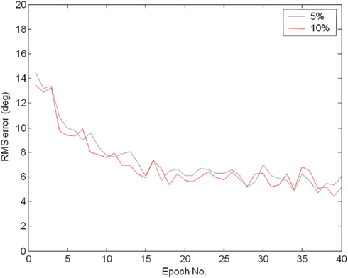
Figure 8. Average RMS error at the end of each epoch, shown for two different learning rates (Eq. 2). A learning rate of 10% generally produces lower error compared to that of the 5% rate at the same epoch, even though the learning progress is not twice as fast.

FIGURE 9

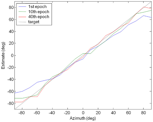
Figure 9. The robot’s progress in localization during training. Initial localization was poor. After 40 epochs of training, its localization ability had greatly improved and accuracy was within 5° at most positions.

FIGURE 10

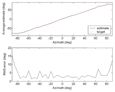
Figure 10. Results of the localization test with a pink noise stimulus, showing the average estimate and RMS error at each position over five trials.

FIGURE 11

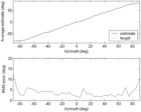
Figure 11. Localization Results for the white noise stimulus. The results were very similar to those for pink noise.

The average RMS errors from both localization tests were calculated and presented in Table 1. Surprisingly, the average error was lower for white noise, even though pink noise was used in training. More importantly, this demonstrated that the system was robust and could localize sound that was different from that encountered during training. The improved performance with white noise is likely due to an improved signal to noise ratio in the higher frequency channels compared to the pink noise stimulus given the background noise in the office environment.

TABLE 1

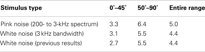
Table 1. Average RMS errors for the two types of stimuli and comparison with previous results.

For comparison, we have included the localization results in a quiet, almost anechoic room from the previous paper (Chan et al., 2010) in Table 1. It could be seen that they were almost identical, even though the acoustic environments were quite different. Despite the presence of noise and reverberation, our system was able to adapt and overcome these non-idealities, localizing sound as well as in the quiet, almost anechoic room.

Experiment 2

The test results from 100 trials are presented in Table 2. The target was correctly identified 75% of the time. The algorithm was not perfect because the onset detector outputs from the audio stimulus and LED 3 were not exactly synchronous (Figure 6) and it was possibly for LED 2 to obtain a better match if it turned on at the right time. These results show that a single onset can be quite ambiguous as the two flashing distractor LEDs alone were generating 50 events per second so that the probability of having “almost simultaneous” onsets was very high. These confusions can be reduced by detecting both the sound onset and the sound offset and correlating these with the onset and offset of the LED. We have not performed this experiment because the vision sensor used (Chan et al., 2007a), which was developed for a different application, was designed to detect onsets only. Changes to the setup of the AER EAR would also be required because the silicon cochlea is currently tuned to give selective band-pass responses, which is optimal for our localization algorithm but not very effective in the detection of sound offset. This can be seen in Figure 2, where the offset time cannot be easily identified from the spike trains.

TABLE 2

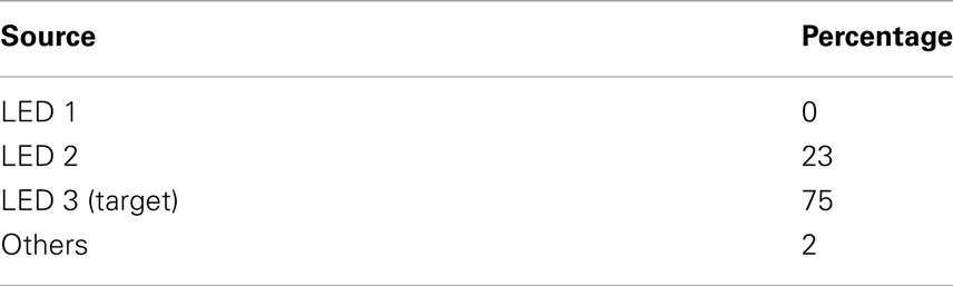
Table 2. Results from 100 trials, showing the percentage that each source is selected.

Conclusion

In this paper, we have demonstrated the training of a robot to localize sound through self motion and visual feedback, by combining an adaptive ITD sound localization system with a transient vision sensor. After training, the robot was able to locate a sound source quite accurately even in the presence of background noise and reverberations. The average RMS error over the [−90°, 90°] range was only 5° for pink noise and 4.4° for white noise. More significantly, the results from the white noise stimuli were almost identical to those from our previous paper, which was conducted in an almost anechoic environment. This demonstrated the importance of learning and adaptation to optimize the performance of a sensory system in the presence of noise and other non-idealities.

In a second experiment, we explored the idea of AV binding and investigated the feasibility of matching audio and visual events based on their onset time. Successful implementation of AV binding can allow a robotic system to adapt and learn based on AV events in the field, without supervision. Our initial experiment showed promising results, with 75% accuracy in the presence of a large number of background events. This indicates matching onset time alone might be sufficient in certain situations where background events occur infrequently. In more complicated environments, however, matching onset time alone is most likely not effective enough to train sound localization using feedback from the visual sensor, which, in the case of our experimental setup, would be systematically wrong 25% of the time. Detecting both the onset and offset of the sound and the LED would likely result in a much lower error rate and allow the unsupervised training to take place.

Conflict of Interest Statement

The authors declare that the research was conducted in the absence of any commercial or financial relationships that could be construed as a potential conflict of interest.

Footnotes

1. ^ ITD stands for interaural time difference.
2. ^ WTA stands for winner-takes-all, a type of feedback network where only the node with the strongest input will generate an output. A soft-WTA relaxes this condition, allowing other nodes with inputs of comparable strength to have non-zero outputs.
3. ^ Although it is possible to update the weights here because we know the actual position of the source, this is not possible when the robot is in the field because the true location of the source must be determined by the robot visually.

References

Becanovic, V., Hosseiny, R., and Indiveri, G. (2004). “Object tracking using multiple neuromorphic vision sensors,” in RoboCup 2004: Robot Soccer World Cup VIII, eds D. Nardi, M. Riedmiller, C. Sammut, and J. Santos-Victor (Berlin: Springer), 426–433.

Bothe, H., Persson, M., Biel, L., and Rosenholm, M. (1999). Multivariate sensor fusion by a neural network model. Fusion’99 Proceedings, Sunnyvale, 2, 1094–1101.

Chan, V., Jin, C., and van Schaik, A. (2007a). An address-event vision sensor for multiple transient object detection. IEEE International Symposium on Circuits and Systems, New Orleans, Vol. 1, 278–288.

Chan, V., Liu, S.-C., and van Schaik, A. (2007b). AER EAR: a matched silicon cochlea pair with address event representation interface. IEEE Trans. Circuits Syst. I Regul. Pap. 54, 48–59.

CrossRef Full Text

Chan, V., Jin, C., and van Schaik, A. (2010). Adaptive sound localization with a silicon cochlea pair. Front. Neurosci. 4:196. doi:10.3389/fnins.2010.00196

CrossRef Full Text

Deiss, S. R. (1994). SCX Project – Address-Event Protocol. Zurich: Institute of Neuroinformatics.

Deiss, S. R., Douglas, R. J., and Whatley, A. M. (1998). “A pulse coded communications infrastructure for neuromorphic systems,” in Pulsed Neural Networks, eds W. Maass and C. M. Bishop (Boston: MIT Press), 157–178.

Gomez-Rodriguez, F., Linares-Barranco, A., Miro, L., Shih-Chii, L., van Schaik, A., Etienne-Cummings, R., and Lewis, M.A. (2007). “AER auditory filtering and CPG for robot control,” in IEEE International Symposium on Circuits and Systems, New Orleans, 1201–1204.

CrossRef Full Text

Hornstein, J., Lopes, M., Santos-Victor, J., and Lacerda, F. (2006). “Sound localization for humanoid robots – building audio-motor maps based on the HRTF,” in IEEE/RSJ Internation Conference on Intelligent Robots and Systems, Beijing, 1170–1176.

CrossRef Full Text

Jimenez-Fernandez, A., Paz-Vicente, R., Rivas, M., Linares-Barranco, A., Jimenez, G., and Civit, A. (2008). “AER-based robotic closed-loop control system,” in IEEE International Symposium on Circuits and Systems, Seattle, 1044–1047.

K-Team. (2008). Koala Robot. K-Team Corporation. Available at: http://www.k-team.com/kteam/index.php?site=1&rub=22&page=18&version=EN

Linares-Barranco, A., Gomez-Rodriguez, F., Jimenez-Fernandez, A., Delbruck, T., and Lichtensteiner, P. (2007). “Using FPGA for visuo-motor control with a silicon retina and a humanoid robot,” in IEEE International Symposium on Circuits and Systems, New Orleans, 1192–1195.

CrossRef Full Text

Mead, C. A. (1989). Analog VLSI and Neural Systems. Boston: Addison-Wesley.

Mead, C. A. (1990). Neuromorphic electronic systems. Proc. IEEE 78, 1629–1636.

CrossRef Full Text

Nakashima, H., Mukai, T., and Ohnishi, N. (2002). “Self-organization of a sound source localization robot by perceptual cycle,” in International Conference on Neural Information Processing, Singapore, Vol. 2, 834–838.

van Schaik, A., and Liu, S.-C. (2005). AER EAR: a matched silicon cochlea pair with address event representation interface. Proc. IEEE Int. Symp. Circuits Syst. 5, 4213–4216.

CrossRef Full Text

Wong, W. K., Neoh, T. M., Loo, C. H., and Ong, P. C. (2008). “Bayesian fusion of auditory and visual spatial cues during fixation and saccade in humanoid robot,” in Proceedings of the 15th International Conference on Advances in Neuro-Information Processing, Auckland, Vol. 1, 1103–1109.