Slow potentials in time estimation: the role of temporal accumulation and habituation

Introduction

Since the early days of EEG research have slow potentials, especially at midline locations, been linked to preparation processes and time estimation (e.g., Walter, 1964). Later research has suggested that the increase in contingent negative variation (CNV) amplitude is a reflection of the internal bookkeeping of the unfolding of time (e.g., Macar et al., 1999). Another phenomenon related to slow potentials in the context of time estimation is that the amplitude of the CNV decreases with increased accuracy or practice (e.g., McAdam, 1966). Although it has been argued that the time estimation-related amplitude effects in the CNV are not sensitive to habituation (Macar and Vidal, 2004), this assumption has not been empirically addressed.

The CNV is a slow negative electrophysiological shift, typically found at fronto-central, central, and parieto-central regions (Walter, 1964), which develops when a subject is expecting an event. The CNV has been associated with many psychological processes such as the preparation for a response and attention (for an early review, see Tecce, 1972), but also, already in some early CNV studies, with interval timing (e.g., Walter, 1964; McAdam, 1966; Weinberg et al., 1974; Ruchkin et al., 1977). Although in many studies the increase in CNV amplitude could also be related to the motor preparation that was required to signal the end of the interval, a series of elegant standard-comparison studies have provided strong evidence for a direct relation between CNV amplitude and cognitive timing (e.g., Pouthas et al., 2000; Macar and Vidal, 2003; Tarantino et al., 2010). In these studies, participants have to compare the duration of events to a previously learned standard duration. If the to-be-compared event takes longer than the standard duration, the CNV shows a positive deflection before the offset of the event, indicating that the CNV is related to the timing of the standard duration. Typically, the link between CNV amplitude and timing is explained within the framework of centralized internal clock theories.

According to the centralized internal clock theories (e.g., Creelman, 1962; Treisman, 1963), a pacemaker generates pulses at a given frequency, which are integrated in an accumulator module. When the duration of an event needs to be timed, the accumulator is set to zero at the onset of the event, and its value is read out at the offset of the event. The number of pulses accumulated can be used as an internal representation of the perceived duration. This internal representation is assumed to be stored in reference memory, and when the duration of the event needs to be reproduced, the system waits until the same amount of pulses have passed (a detailed model of this process is discussed in Taatgen and Van Rijn, 2011). This general outline has been very influential and multiple theories are essentially implementations of this basic idea (e.g., the scalar expectancy theory, SET; Gibbon, 1977; Gibbon and Allan, 1984; Wearden, 1991; the attentional-gate models, Zakay and Block, 1997; and the integrated time models, Taatgen et al., 2007; Van Rijn and Taatgen, 2008).

The pacemaker–accumulator models rely on the concept of accumulation as all decisions depend on the number of accumulated pulses. Given the similarities between the increasing negativity of the CNV and the increasing value of the accumulator over time, it has been suggested that the CNV reflects the accumulation process. This assumption also explains the coincidence between the CNV peak and the standard duration in temporal generalization or standard-comparison studies: The accumulator, reflected in the CNV, stops its activity when the currently unfolding duration equals the memorized standard. Although the simplest assumption is that the observed CNV is a direct reflection of the value currently stored in the accumulator, an alternative explanation could be that the CNV reflects the unfolding of time in a more indirect way, for example by expressing the difference between the current time and the earlier perceived durations.

The most powerful empirical argument in favor of a more direct link between pulse accumulation and the CNV was provided by Macar et al. (1999). Given the assumption that trial-to-trial fluctuations in temporal performance are driven by differences in the current state of the accumulator, the observed fluctuations in behavioral responses should correlate with the measured CNV amplitude. Macar et al. (1999) tested this assumption of performance-dependent variations in the CNV amplitude by asking their participants to produce an earlier learned standard duration of 2.5 s by pressing a key twice. Trials were post hoc categorized into three groups: a group of “short” productions (2.2–2.4 s), of “correct” productions (2.4–2.6 s), and of “long” productions (2.6–2.8 s). The (Laplacian-based) CNV measured at the FCz electrode was compared for the three conditions. In line with their assumption that the buildup in the accumulator is reflected in the CNV, Macar et al. (1999) found a higher CNV amplitude in the long condition, an intermediate CNV amplitude in the correct condition, and a lower CNV amplitude in the short condition. The positive correlation between produced duration and CNV amplitude strongly suggests that the unfolding of time – and thus the value of the accumulator – is directly linked with the amplitude of the CNV. Of course, if one assumes a relative stable threshold in this well-trained interval production task, this interpretation hinges on the notion that participants failed to notice that the accumulator already reached the threshold in the long condition, and that participants responded before the accumulator reached the threshold in the short condition. This idea, and especially the assumption of a response well before the threshold is reached (see Figure 2 of Macar et al., 1999), is of course problematic from the perspective of the pacemaker–accumulator theories since these theories are based on the assumption that responses are triggered by the accumulator reaching the threshold. However, a similar finding was reported by Macar and Vidal (2002) in a study that focused on memory consolidation in time perception: Trials in which the interval was overestimated were associated with more negative CNV amplitudes.

Another phenomenon related to the amplitude of the CNV that has been known since the onset of EEG research is the habituation effect. McAdam (1966) demonstrated that the CNV amplitude changes over the course of an experimental session, with a lower amplitude during the later phases. McAdam (1966) related this habituation effect to higher accuracy, a finding that was supported by Ladanyi and Dubrovsky (1985) who reported lower CNV amplitudes for a group of accurate time estimators compared to a group of participants who over estimated the interval. Similar effects were reported by Macar and Vitton (1979) on the basis of a study in which cats were subjected to a schedule of temporal conditioning: with prolonged training, the observed negativity decreased. Taken together, these data has been interpreted that CNV habituation serves as an index of gradual automation of time processing (e.g., Pfeuty et al., 2003; Pouthas, 2003).

If, however, this habituation effect also played a role in the Macar et al. (1999) experiment, the observed effects might be partly due to a habituation-based decrease of amplitude. That is, if participants initially slightly overestimated the durations and improved during the experimental session, the initial trials will have a higher chance of being categorized as “long” than the later trials. Combined with a decrease in amplitude during the experiment due to habituation, this might have emphasized a correlation between estimated durations and CNV amplitude.

Given the importance of the Macar et al. (1999) results for the hypothesis that the CNV reflects the unfolding of time, we have conducted two replication experiments to assess the contributions of performance-dependent variations in, and the effect of habituation on the CNV amplitude.

Materials and Methods

Both experiments reported here were run as the first part of two larger experiments on the effects of attention on time estimation. In this paper, we will only report on the first part of the experiments, which was set up as a replication of the study reported by Macar et al. (1999). Participants were, while performing the here reported study, not instructed on the later parts of the experiment.

We will discuss the materials and methods for both experiments before turning to the discussion of the results.

Experiment 1

Task

The participants were asked to produce a 2.5-s interval by pressing the spacebar twice. Feedback was presented after each trial indicating the deviation from the learned standard. During the entire interval a small circle (about 1 cm in diameter) served as a fixation point. Before the first key press, the circle was shown in light gray on a black background. The first key press changed the color of the circle to white, as a visual cue that the interval had started. The second key press removed the circle from the screen, and after 200 ms feedback was presented for a duration sampled from a uniform distribution between 1 and 1.5 s. The feedback was delivered as a row of five circles, immediately above the location of the fixation point. If the time production was “perfect” (between 2.4 and 2.6 s), the middle circle turned green. If time production was between 1.8 and 2.4 s or between 2.6 and 3.2 s, the circle just to the left or right of the middle circle turned green. If the time production was shorter than 1.8 or longer than 3.2 s, the left or right outer circle turned red. See Figure 1 for a graphic depiction of the feedback screen. Participants were instructed that appearance of a red circle indicates a “too short” or “too long” time production, and that they should aim for as precise as possible temporal performance. Before each trial, a “Please blink” instruction was presented for 500 ms to reduce blinks during the time production trials.

FIGURE 1

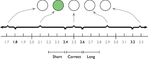
Figure 1. The horizontal row of five circles depict an example feedback screen. The green circle indicates the participant that the produced interval was too short. The time line indicates the ranges associated with particular feedback circles. The three pseudo-experimental conditions as defined by Macar et al. (1999) on which the ANOVA analyses are based are illustrated below the timeline.

Procedure

Experiment 1 consisted of a training and an experimental block. In the training block, participants were asked to learn the 2.5-s interval by adjusting their productions based on feedback. After producing three time productions between 2.4 and 2.6 s in succession, the training block was considered finished, and the experimental block started. The maximum length of the training block was set to 50 trials. The length of the experimental block was dynamically adjusted, as it lasted until 252 time productions between 1.8 and 3.2 s were obtained. Participants were instructed to use the feedback to estimate the interval as accurately as possible and to not use external timing strategies such as counting or foot tapping. Participants were allowed to take a break whenever necessary.

Participants

Twenty-two Psychology students participated in the experiment and received partial course credit. All participants had normal or corrected-to-normal visual acuity. Informed consent as approved by the Ethical Committee Psychology of the University of Groningen was obtained before testing. Nine subjects (mean age: 21.3, range: 20–25, 6 females) fulfilled the “3-in-a-row” criterion as set by Macar et al. (1999). Although this inclusion rate is rather low (approximately 40%), Macar et al. (1999) reported that they preselected their participants based on performance in other timing tasks. Here we did not apply any pre-selection criteria, which might explain the low inclusion criteria. Of the remaining participants, eight showed behavioral performance during the experimental phase that was similar to the “3-in-a-row” participants (i.e., needed less than 280 trials to achieve 252 time productions between 1.8 and 3.2 s). We will also report analyses on the extended dataset of 17 participants.

Electrophysiological recordings

Electrical brain activity was recorded from 30 scalp locations (AFz, F5, F3, F1, Fz, F2, F4, F6, FC5, FC3, FC1, FCz, FC2, FC4, FC6, C5, C3, C1, Cz, C2, C4, C6, CP3, CP1, CPz, CP2, CP4, P3, Pz, P4). Vertical and horizontal EOG activity and both mastoids were registered. For all channels Ag–AgCl electrodes were used and impedances were kept below 5 kΩ. Using the Refa system (TMS International B.V.), all channels were amplified and filtered with a digital FIR filter with a cutoff frequency of 135 Hz (low pass) and were recorded with a sampling rate of 500 Hz using Portilab (TMS International B.V.). Using BrainVision (Brain Products GmbH), the signals were referenced to the mastoids and a 50-Hz notch filter was applied to reduce line noise artifacts.

Data preprocessing and analysis

Parameters for data preprocessing were set to be as similar as possible to the settings reported by Macar et al. (1999). The average voltage over the first 100 ms preceding the first key press was used as baseline for second key press-locked plots and analyses, and the average voltage between 1 and 0.9 s preceding the first key press was used as baseline for first key press-locked plots and analyses. Trials in which the maximum absolute amplitude exceeded 100 μV or in which the amplitude range exceeded 150 μV were discarded. Eye blinks were corrected using the Gratton and Coles method (Gratton et al., 1983). Data were filtered offline with a bandpass of 0.01–100 Hz with 12 dB/Oct slope. Trials containing ocular artifacts, movement artifacts, or amplifier saturation were excluded from further processing by visual inspection. We will report on data from the FCz electrode both on monopolar electrophysiological activity and data obtained after Laplacian transformation (Hjorth, 1975). Note that Hjorth (1975) advocates the use of 5-point operator derivations (which, in our case, would involve AFz, CPz, FC3, and FC4), but to keep the reported analyses as similar as possible to the ones reported by Macar et al. (1999), we computed the Laplacians using the same triangular configuration (F3, F4, CPz) as presented by Macar et al., 1999; Figure 1) see Vidal et al. (2003), for more details on this method). However, informal comparisons between the triangular configuration and the 5-point operator derivations did not indicate that the interpretation of the data hinged on which method was chosen. As described in Vidal et al. (2011), we averaged the monopolar recordings that remained after artifact correction and rejection, and calculated the Laplacians on the basis of these monopolar averages [by using the formula {3xFCz − (F3 + F4 + CPz)}/distance², with distance equal to 7 cm]. Statistical tests on the average amplitude were computed for the interval that ranges from 1500 to 100 ms before the second key press that ended the time production. We will report Laplacian-based analyses for both the “3-in-a-row” and the extended group, and analyses on monopolar data for the extended group to provide additional insight.

Experiment 2

Task

In comparison to the procedure of Experiment 1, (1) the delay between the second response of the participant and the presentation of the feedback was increased from 200 to 500 ms, (2) the “please blink” instruction at the start of each trial was removed, and (3) the inter-trial delay was sampled from a uniform distribution with a range of 1500–3000 ms. These settings were chosen to better match the Macar et al. (1999) setup. All other details were left unchanged.

Procedure

In comparison to the procedure of Experiment 1, the maximum length of the training block was extended from 50 trials to 90 trials. All other details were left unchanged.

Participants

Twenty-four Psychology students participated in the experiment and received partial course credit. Eight participants (age: 22.9, range 19–31, 6 females) fulfilled the same “3-in-a-row” correct criteria as used in the Macar et al. (1999) experiment. We again did not apply any pre-selection criteria. Another seven participants performed equally well during the experimental phase (less than 280 trials to achieve 252 time productions between 1.8 and 3.2 s) and were included in the analyses on the extended dataset.

Electrophysiological recordings

Data was recorded using the same setup as used for Experiment 1 from the following scalp locations: AF3, AFz, AF4, F3, Fz, F4, FC3, FC1, FCz, FC2, FC4, C3, C1, Cz, C2, C4, CP3, CPz, CP2, CP4, P3, P1, Pz, P2, P4, PO3, POz, PO4, O1, Oz, and O2.

Data preprocessing and analysis

Preprocessing and analysis procedures were identical to those reported for Experiment 1.

Results

Experiment 1: ANOVA-Based Results

All analyses reported in this section are based on the pseudo-experimental categorization used by Macar et al. (1999), as depicted in Figure 1. Data were subjected to repeated measures analyses of variance (ANOVA).

The length of the training session depended on the subject’s performance, and lasted between 10 and 49 trials for the “3-in-a-row” group. Macar et al. (1999) reported that the successful training criterion was reached after 16–55 trials in their experiment. Each averaged ERP waveform (i.e., per participant and per pseudo-experimental group) contained at least 30 and at most 115 trials, with an average of 55 trials. After preprocessing of electrophysiological data, the produced intervals were sorted into 0.2-s categories. Three categories, designated as “short” (2.2–2.4 s), “correct” (2.4–2.6 s), and “long” (2.6–2.8 s), served as pseudo-experimental conditions. Overall, 65% of the trials were included: 19% correct, 27% short, and 19% long. About 31% of all trials resulted in temporal productions outside the range of the pseudo-experimental groups, and 4% of all trials were rejected. On average, participants needed 267 trials to get at 252 correct trials. Performance for the eight participants who did not meet the “3-in-a-row” criterion was similar.

Performance-dependent variations

Figure 2 provides the Laplacian data during the 1-s period preceding a first button press. We did not find any differences during the 100-ms period prior to the first key press, nor for an extended period of 500 ms prior to the first key press (Fs < 1). Figure 3 shows the second key press-locked averages for the three pseudo-experimental conditions. Analyses on the average Laplacian amplitudes (from 1.5 to 0.1 s before the second key press) showed no effect of pseudo-experimental groups for the FCz electrode for the “3-in-a-row” group (F < 1) nor for the extended group [F(2,34) = 1.2, p = 0.32]. The monopolar data for the extended group did not show any significant results either (F < 1).

FIGURE 2

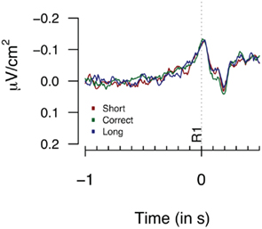
Figure 2. Laplacians obtained at FCz during Experiment 1 as a function of participants’ behavioral performance, plotted time-locked to the first key press (R1). Averages are based on nine participants who met the “3-in-a-row” criterion.

FIGURE 3

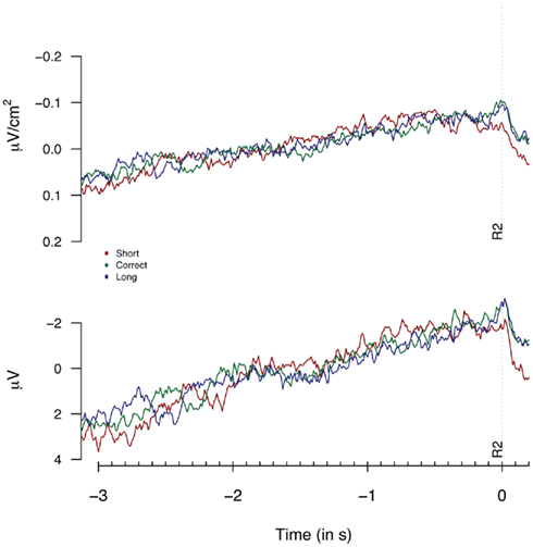
Figure 3. Laplacians (top graph) and monopolar recordings (bottom graph) obtained at FCz during Experiment 1 as a function of participants’ behavioral performance, plotted time-locked to the second key press (R2). Laplacians are based on 9 “3-in-a-row” participants, monopolar data are based on the extended dataset consisting of 17 participants.

Thus, neither the analysis based on monopolar nor on Laplacian-transformed data replicated the performance-dependent variations as reported by Macar et al. (1999).

Habituation effects

To check the presence of habituation effects in our data, the same trials as analyzed for the performance-dependent variations (i.e., time productions between 2200 and 2800 ms) were sorted into three equally sized groups based on the sequential order of trials during the experimental block. Figure 4 shows the Laplacian and the monopolar traces for the three groups. The most elegant analysis would include factors for both habituation effects and performance-dependent variations, however, the number of observations per cell would differ too much in such a setup to allow for reliable tests based on cell means. Therefore, we will analyze habituation effects independently from performance-dependent variations. Note that we will discuss analyses on monopolar data in Section “Linear-Mixed Effect Model-Based Analysis of Experiment 1 and 2” that include both habituation and performance-dependent variations in a single analysis.

FIGURE 4

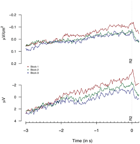
Figure 4. Second response (R2) locked Laplacians (top graph, means based on 9 “3-in-a-row” participants) and monopolar recordings (bottom graph, means based on 17 participants) obtained at FCz during Experiment 1, plotted separately for the first, second, and third 33% of all trials.

A repeated measures ANOVA on monopolar data for all participants (shown in Figure 4), showed significant effects, not only at FCz [F(2,34) = 4.0, p = 0.02] but at a broad range of fronto- and fronto-central electrodes: F1: F = 5.8; Fz: F = 3.5: F2: F = 4.2; FC1: F = 3.1; FC2: F = 3.6 and Cz = 3.9, all df(2,34); all p < 0.05. The analysis of Laplacian data failed to reach significance [F < 1 and F(2,34) = 1.17, p = 0.3 for the “3-in-a-row” and for all participants respectively]. However, visual inspection of Figure 4 shows signatures of habituation effects for FCz in both monopolar and in Laplacian-transformed data, suggesting that the lack of effect in the Laplacian-transformed data might be related to the limited power of an analysis based on three categorial groups.

Given that these analyses are also based on differences in amplitude, it is even more surprising that we were unable to replicate the performance-dependent CNV amplitude effects. Because of some slight differences between the original study by Macar et al. (1999) and our Experiment 1, and to check the consistency of our results, we ran another replication study. The most important modification was the extension of the training block from 50 to 90 trials as in the Macar et al. (1999) experiment. Note that we originally set the training block to 50 trials as behavioral pilot studies showed that no extensive improvement in temporal accuracy was obtained after 50 trials.

Experiment 2: ANOVA-Based Results

The length of the training block depended on the subject’s performance as the experimental block started as soon as a subject produced three trials in a row between 2.4 and 2.6 s. Participants who met this criterion needed between 30 and 58 trials, with only a single participant needing more than 50 trials. This level of performance is very similar to our Experiment 1 and to the Macar et al. (1999) study. Each averaged ERP waveform (i.e., per participant and per pseudo-experimental group) contained at least 30 and at most 92 trials, with an average of 54 trials. After preprocessing of electrophysiological data, 64% of all trials were included in the three specified pseudo-experimental groups: 22% in short, 26% in correct, and 16% in long. About 23% of all trials resulted in temporal productions outside the range of the pseudo-experimental groups, and 13% of all trials were rejected because of artifacts. On average 260 trials were needed to get at 252 correct trials.

Performance-dependent variations

Figure 5 provides the Laplacian data during the 1-s period preceding a first button press. We did not find any differences during the 100 or 500-ms period prior to the first key press [F(2,14) = 1.82, p = 0.3; F(2,14) = 1.23, p = 0.19 respectively]. The second key press-locked Laplacian data presented in Figure 6 showed no effect for performance-dependent variations in CNV [F(2,14) = 2.62, p = 0.108; F(2,28) = 2.68, p = 0.086, for the “3-in-a-row” and for all participants respectively]. Note that the relatively big F values are driven by an opposite-to-expected order in CNV amplitudes, with short associated with the highest amplitude. The monopolar recordings did not reveal any significant effect (F < 1).

FIGURE 5

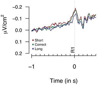
Figure 5. Laplacians obtained at FCz during Experiment 1 as a function of participants’ behavioral performance, plotted time-locked to the first key press (R1). Averages are based on eight participants.

FIGURE 6

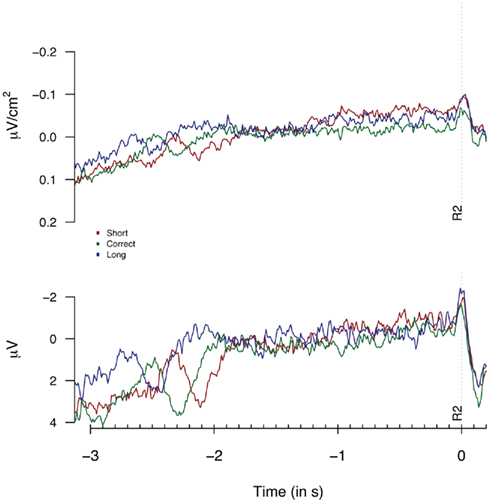
Figure 6. Laplacians (top graph) and monopolar recordings (bottom graph) obtained at FCz during Experiment 2 as a function of participants’ behavioral performance, plotted time-locked to the second key press (R2). Laplacians are based on 8 “3-in-a-row” participants, monopolar data are based on all 15 participants.

Habituation effects

As for Experiment 1, we tested for the presence of habituation effects. Figure 7 shows the Laplacian-transformed and monopolar traces plotted separately for the first, second, and third 33% of all trials. No habituation effects for Laplacian and monopolar data reached significance (Fs < 1).

FIGURE 7

Figure 7. Second response (R2) locked Laplacians (top graph, eight “3-in-a-row” participants) and monopolar recordings (bottom graph, all participants) obtained at FCz during Experiment 2 plotted separately for the first, second, and third 33% of all trials.

Linear-Mixed Effect Model-Based Analysis of Experiment 1 and 2

The analyses reported above are based on a post hoc categorization of the participants’ responses. This categorization allows for comparing the amplitudes of short, correct, and long trials by means of traditional ANOVA. We have reported these as similar analyses are reported by Macar et al. (1999). However, the premise that variations in estimated durations correlate with the observed CNV amplitude at FCz should also hold if the actual durations are correlated with the amplitude, instead of comparing means based on aggregation in three bins. However, given the distribution of durations, increasing the number of bins and performing ANOVA-style analyses would likely violate the assumptions underlying an ANOVA. The same issue prevents doing analyses in which the effects of performance-based variations are tested simultaneously with habituation effects. As argued earlier, it might be that the habituation effects either artificially strengthen or conceal the effects of the performance-based variations, or vice versa.

An alternative type of analysis that allows for entering the raw durations of multiple factors instead of binned duration-categories are linear-mixed effects models (e.g., Pinheiro and Bates, 2000; Gelman and Hill, 2007; Baayen, 2008). These models allow for testing the effect of multiple continuous (pseudo-) experimental manipulations while taking the (repeated measures) structure of the design into account.

To improve on the power of the analyses, we will here report linear-mixed effect model-based analyses for just the monopolar data. As the reported Laplacians are based on averages (c.f., Macar et al., 1999), no trial-by-trial information is available. Therefore, we cannot report linear-mixed effect models on the Laplacian-transformed data but analyses based on spherical spline current source density (Perrin et al., 1989) transformations showed similar results to the monopolar data presented here. We will analyze both Experiment 1 and Experiment 2 separately, including just those participants who met the “3-in-a-row” criterion, but also perform a combined analysis in which we include participants from the extended groups of both Experiment 1 and 2.

Figure 8 shows the result of the linear-mixed effect model in which the monopolar average amplitude (calculated over 1.5–0.1 s before the second response, similar as for the ANOVA-based analyses) was entered as the dependent variable. All trials in which the absolute average amplitude exceeded 50 μV were removed. Both duration, a factor representing the effect of the performance-based variations, and habituation, a factor representing the overall time course of the experiment were entered as fixed factors. In addition to these fixed factors, we allowed for a random intercept per participant, and independent random effects for duration and habituation per participant. The factor duration was calculated by subtracting 2.5 s from the observed behavioral durations. The estimated effects for duration thus represent the change in microvolt per 1 s deviation from 2.5 s. Habituation is expressed as a function of trial number, with the first trial of each participant coded as 0, and the last trial as 1. Each of the dots represent the Markov Chain Monte Carlo-based estimated coefficient (Baayen, 2008) for the effect of that factor for each participant. The blue and red colored dots represent the participants who met the “3-in-a-row” criterion and who participated in Experiment 1 and Experiment 2 respectively. The gray dots represent the participants from both experiments who met the more relaxed criterion for inclusion in the extended dataset. As can be seen in Figure 8, the estimated effects of these extended group participants are similar to those of the “3-in-a-row” group. Therefore, we will focus the discussion on the overall analyses, represented by the black means and error bars (although the same information is available for the two subsets, color-coded in blue and red). The mean with the error bars denotes the overall effect of that factor and the 95% highest posterior density-based confidence intervals.

FIGURE 8

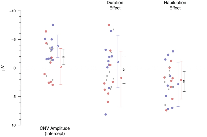
Figure 8. Estimated monopolar-based effects for the CNV amplitude, the performance-based variations (Duration) and the habituation effect. Circles represent individual participants, mean and SE lines represented the estimated effect and HPD 95% confidence intervals. Blue represents Experiment 1, red Experiment 2, and the gray circles represent the participants who did not meet the “3-in-a-row” criterion. The black means and confidence intervals represent the overall analysis.

The monopolar-based linear-mixed effect model largely confirms the conclusions drawn from the ANOVA-based analyses. First, the overall model contains a negative intercept, reflecting the typical CNV effect (β = −1.92, p < 0.001). Second, we again found no indication of an effect of performance-based variations in CNV amplitude (β = 0.32, p = 0.81). Third, the overall habituation effect reaches significance (β = 2.40, p = 0.008), indicating that the negativity associated with the CNV is attenuated during the course of the experiment. Adding a Duration times Habituation interaction term does not improve the fit of the model to the data (χ² = 0.08, df = 1, p = 0.77).

The habituation effect observed at FCz is not in line with Macar and Vidal (2004) suggestion that time estimation-related amplitude effects in the CNV are not sensitive to habituation. However, it might be that these effects are epiphenomena of an ongoing learning process that results in attenuation of the CNV over time. A signature of such a learning process would be an increased accuracy in temporal productions over the time course of the experiment. To test for learning, we assessed whether the absolute deviation of the standard decreased during the experiment. However, a linear-mixed effect model with absolute deviation from the standard as the dependent variable and trial number rescaled to a 0.1 range as fixed factor and subject as random factor did not show an effect of trial number (β = −0.005, HPD 95%: −0.021 0.011, p = 0.519, based on 10000 Markov chain Monte Carlo samples), which indicates that we failed to find any evidence in favor of participants still improving their estimations during the scope of the experiment.

To summarize, even the more powerful linear-mixed effect analysis did not provide any evidence in favor of the hypothesis that the duration of produced intervals correlate with the associated CNV amplitudes, while this analysis did find support for habituation effects.

Discussion

It has been hypothesized that the CNV amplitude measured at the FCz electrode, which is assumed to measure supplementary motor area (SMA)-related activity, reflects an online temporal accumulation of the currently unfolding time interval (Macar et al., 1999; Macar and Vidal, 2002). Based on experimental data, Macar et al. (1999) concluded: “this region, which mainly includes the SMA, contains the temporal accumulator described in prominent models of time processing” or, “[a]lternatively, through thalamic relays, it may receive output from a temporal accumulator located in striatal structures” (p. 278). These conclusions, and especially the stronger conclusion that the activity in the SMA indicates to how much time has passed since the onset of an interval of course predicts a stable correlation between performance and observed CNV variations. However, early work on the brain correlates of time estimation showed that CNV decreased over the time course of the experiment, often referred to as habituation (McAdam, 1966; Ladanyi and Dubrovsky, 1985). In two experiments, we have tested whether we could replicate these contradictory results.

However, neither in Experiment 1, nor in Experiment 2, nor in the combined analyses of all data did we find any systematic or consistent performance-based variations in the CNV amplitude. At the same time, we did find evidence in favor of the habituation effect in the linear-mixed effect analyses, indicating that the CNV amplitude decreases as a function of the time course of the experiment as was reported by earlier work (McAdam, 1966; Ladanyi and Dubrovsky, 1985; Pfeuty et al., 2003).

As we set out in the introduction, the performance-based variations might have been enhanced (or attenuated) by an interaction with the habituation effects if the behavioral data would have showed a progressive shortening of the estimated intervals over the time course of the experiment. Although we had to perform the ANOVA-based analyses separately for the habituation effect and for the performance-dependent variations, the linear-mixed effect model-based analyses contained both components in a single analysis which would have allowed for testing whether habituation effects might influence the performance-based variations. Since we did not find any performance-based amplitude effects, this hypothesis cannot be fully assessed.

Of course, as these results are in stark contrast to the results reported by Macar et al. (1999) the question arises what causes these differences. Given that we did find the expected CNV effect, effects of habituation, and typical ERPs, it is likely that we would have observed signatures of performance-dependent variations if at all present in this data. However, inspection of Figure 8 shows large individual differences for the estimated effect of performance-dependent variations. This variability does suggest that if a small number of participants is tested, a Type I error might result. The probability of both Type I and Type II errors are also increased when discretized data is used in an analysis based on cell means, for example because the mean of a category can be strongly influenced by an extreme observation (see, for example, Royston et al., 2006; Wainer et al., 2006). Note that the ANOVA-based analyses reported by Macar et al. (1999) and replicated in this paper are based on discretized data and cell means, and as such might be biased, but that the linear-mixed effect analyses are not affected.

Another potential source of differences between our and Macar et al.’s (1999) work are the participant inclusion rates. Although the exact proportion of participants not meeting the “3-in-a-row” criterion is not reported in Macar et al. (1999), Vidal (personal communication, January 11, 2011) has indicated that their exclusion rate was quite a bit lower than the high exclusion rates observed for our two experiments. On the basis of this difference, one could argue that even the participants who met the “3-in-a-row” criterion in our experiments are in some aspects different from the participants tested by Macar et al. (1999) for example, because our participants might have been less motivated. However, this reasoning implies that the participants who met the “3-in-a-row” criterion are more similar to the participants tested by Macar et al. (1999) than the subset of participants who did not meet the “3-in-a-row” criterion. This hypothesis is not supported by the data, as visual inspection of Figure 8 does not indicate any difference in the distributions of the blue/red colored circles versus the gray circles. We, therefore, consider it unlikely that the differences between Macar et al. (1999) and our experiments are purely due to differences in the participant groups.

To summarize, although we report on data of three times the number of participants as analyzed by Macar et al. (1999) and have analyzed the data with more powerful statistical techniques, we failed to replicate the performance-based variations. As discussed in the next paragraph, the literature provides more examples showing that the link between the SMA and the accumulator is not straightforward.

Besides the work presented by Macar et al. (Macar et al., 1999; Macar and Vidal, 2002) results obtained in monkeys during single-cell recording from the SMA and pre-SMA may be interpreted in favor of the performance-dependent variations hypothesis (Akkal et al., 2004; Mita et al., 2009). However, if one assumes that the slow cortical potentials measured at SMA/FCz reflect time accumulation processes, and one assumes that increased CNV amplitudes for longer intervals arises from increased activation of neural structures involved in timing (Macar et al., 1999; Macar and Vidal, 2004), then one should find similar effects in other paradigms where intervals of different durations are estimated. However, this is not regularly reported. For example, in an experiment in which subjects had to reproduce just perceived intervals selected from a 1 to 8-s range, no amplitude differences were observed (Elbert et al., 1991). A similar lack of results was reported for the amplitudes associated with estimations of intervals up to 6 s, even after CSD-based transformations (Gibbons and Rammsayer, 2004). Recently, an alternative explanation has been put forward that assumes that the accumulation in the CNV represents accumulation to a threshold, with the final value of the accumulator to be more or less constant over all trials (assuming a constant threshold). This idea, expressed in the work of Durstewitz (2003, 2004), does not predict amplitude differences for short and long productions, and has found support in timing paradigms (Pfeuty et al., 2005) and serial choice reaction time tasks (Praamstra et al., 2006). Moreover, Balci and Simon (submitted) have presented a drift–diffusion model that builds on the work of Simen et al. (2011) that explains temporal bisection variability in terms of accumulation to a fixed threshold. Since performance-dependent variations were not observed in our study, this data is more in line with the view that the SMA is related to the decision process instead of to the actual accumulation of temporal information.

Interestingly, recent work by Van Maanen and Forstmann (Forstmann et al., 2008; Van Maanen et al., submitted) might reconcile the paradox between the findings of Macar et al. (1999) and our experiments. Forstmann et al. (2008) has demonstrated the pre-SMA and striatum show increased levels of activation when decisions need to be made under time pressure in a speed–accuracy tradeoff experiment. Based on trail-by-trial analyses, Van Maanen et al. (submitted) have shown that this effect is driven by a positive correlation between fluctuations in response caution and the hemodynamic response in pre-SMA and dorsal anterior cingulate. However, this effect was only found when participants were instructed to value speed-over-accuracy. When participants were instructed to value accuracy over speed, Van Maanen et al. (submitted) found no such correlation. If participants respond later if they are more cautious (as in non-temporal tasks), the paradox might be explained by assuming that the participants in the Macar et al. (1999) study performed as in the speed-over-accuracy condition of Van Maanen et al.’s (submitted) study, whereas the participants in our study might have performed as in the accuracy-over-speed condition. Of course, response speed and accuracy cannot be considered independently in an interval timing task where the response latency determines accuracy. However, in the studies by Forstmann et al. (2008) the speed–accuracy manipulations are considered to be a proxy of response caution, which might differ between individuals in an interval timing task. Moreover, Forstmann et al. (2008) showed that individual variation in the activation of striatum and pre-SMA is selectively associated with individual variation in behavior, supporting the notion that the paradox might be explained by different levels of response caution. However, this explanation is also based on the notion that the activity measured at (pre-)SMA is not a direct reflection of the unfolding of time, but a signature of the decision processes involved in interval timing.

Earlier work has identified a relation between levels of brain activity at prefrontal sites with temporal performance, with decreased activation associated with increased temporal performance (Casini et al., 1999), but this habituation effect was not observed at SMA. Based on this result it was hypothesized that “the activity from the SMA is resistant to the habituation because it indexes the increasing efficiency of temporal coding mechanisms with learning, which implies enhanced precision and stability, whereas the prefrontal activity anterior to the SMA rapidly diminishes due to the decreasing load of attentional effort and of possibly interfering mental strategies” (Macar and Vidal, 2004, p. 100). In contrast to the suggested habituation-resistant activity in the SMA, we found habituation effects in the monopolar data.

To conclude, this paper adds to the current discussion on the role of the SMA in time estimation, mainly focusing on the question whether the SMA incorporates or reflects the accumulator as expressed in information-processing models of time estimation, or whether its activity reflects a more indirect component of time estimation tasks such as comparisons to previous experiences or thresholds (see for a discussion, Coull et al., 2010). Where some EEG and fMRI studies link SMA activity to the accumulation of time units during the unfolding of time (e.g., Macar et al., 1999; Coull et al., 2004), other studies have linked similar activity to the indirect processes such as comparison to memorized time intervals (e.g., Pfeuty et al., 2003; Cui et al., 2009). If this latter view is correct, one might expect to see a decrease of CNV amplitude over the course of the experiment, since habituation has typically been related to increased neural proficiency (e.g., McAdam, 1966; Ladanyi and Dubrovsky, 1985; Pouthas, 2003). Given that our analyses did not result in any performance-dependent CNV amplitude variations but did show habituation effects, this data supports the view that the buildup of SMA activity during temporal processing reflects a more indirect process than the direct link between SMA activity and accumulation as proposed by Macar et al. (1999).

Conflict of Interest Statement

The authors declare that the research was conducted in the absence of any commercial or financial relationships that could be construed as a potential conflict of interest.

Acknowledgments

The authors would like to thank Tobias Navarro Schröder for assisting with the data collection, Paolo Toffanin and Mark Span for assistance with setting up the experiment and analyzing the data, and the members of the cognitive modeling group for their useful comments. This work has been supported by the European project COST ISCH Action TD0904 “Time In MEntaL activitY: theoretical, behavioral, bioimaging, and clinical perspectives” (TIMELY; www.timely-cost.eu).

References

Akkal, D., Escola, L., Bioulac, B., and Burbaud, P. (2004). Time predictability modulates pre-supplementary motor area neuronal activity. Neuroreport 15, 1283–1286.

Pubmed Abstract | Pubmed Full Text | CrossRef Full Text

Baayen, R. H. (2008). Analyzing Linguistic Data: A Practical Introduction to Statistics Using R. Cambridge: Cambridge University Press.

Casini, L., Macar, F., and Giard, M. H. (1999). Relation between level of prefrontal activity and subject’s performance. J. Psychophysiol. 13, 117–125.

CrossRef Full Text

Coull, J. T., Cheng, R. K., and Meck, W. H. (2010). Neuroanatomical and neurochemical substrates of timing. Neuropsychopharmacology 36, 3–25.

Pubmed Abstract | Pubmed Full Text | CrossRef Full Text

Coull, J. T., Vidal, F., Nazarian, B., and Macar, F. (2004). Functional anatomy of the attentional modulation of time estimation. Science 303, 1506–1508.

Pubmed Abstract | Pubmed Full Text | CrossRef Full Text

Creelman, C. D. (1962). Human discrimination of auditory duration. J. Acoust. Soc. Am. 34, 582–593.

CrossRef Full Text

Cui, X., Stetson, C., Montague, P. R., and Eagleman, D. M. (2009). Ready...go: amplitude of the FMRI signal encodes expectation of cue arrival time. PLoS Biol. 7, e1000167. doi: 10.1371/journal.pbio.1000167

CrossRef Full Text

Durstewitz, D. (2003). Self-organizing neural integrator predicts interval times through climbing activity. J. Neurosci. 23, 5342–5353.

Pubmed Abstract | Pubmed Full Text

Durstewitz, D. (2004). Neural representation of interval time. Neuroreport 15, 745–749.

Pubmed Abstract | Pubmed Full Text | CrossRef Full Text

Elbert, T., Ulrich, R., Rockstroh, B., and Lutzenberger, W. (1991). The processing of temporal intervals reflected by CNV-like brain potentials. Psychophysiology 28, 648–655.

Pubmed Abstract | Pubmed Full Text | CrossRef Full Text

Forstmann, B. U., Dutilh, G., Brown, S., Neumann, J., Von Cramon, D. Y., Ridderinkhof, K. R., and Wagenmaker, E. J. (2008). Striatum and pre-SMA facilitate decision-making under time pressure. Proc. Natl. Acad. Sci. U.S.A. 105, 17538–17542.

Pubmed Abstract | Pubmed Full Text | CrossRef Full Text

Gelman, A., and Hill, J. (2007). Data Analysis Using Regression and Multilevel/Hierarchical Models. New York: Cambridge University Press.

Gibbon, J. (1977). Scalar expectancy theory and Weber’s law in animal timing. Psychol. Rev. 84, 279–325.

CrossRef Full Text

Gibbon, J., and Allan, L. (1984). Timing and Time Perception. New York: New York Academy of Sciences.

Gibbons, H., and Rammsayer, T. H. (2004). Current-source density analysis of slow brain potentials during time estimation. Psychophysiology 41, 861–874.

Pubmed Abstract | Pubmed Full Text | CrossRef Full Text

Gratton, G., Coles, M. G., and Donchin, E. (1983). A new method for off-line removal of ocular artifact. Electroencephalogr. Clin. Neurophysiol. 55, 468–484.

Pubmed Abstract | Pubmed Full Text | CrossRef Full Text

Hjorth, B. (1975). An on-line transformation of EEG scalp potentials into orthogonal source derivations. Electroencephalogr. Clin. Neurophysiol. 39, 526–530.

Pubmed Abstract | Pubmed Full Text | CrossRef Full Text

Ladanyi, M., and Dubrovsky, B. (1985). CNV and time-estimation. Int. J. Neurosci. 26, 253–257.

Pubmed Abstract | Pubmed Full Text | CrossRef Full Text

Macar, F., and Vidal, F. (2002). Time processing reflected by EEG surface Laplacians. Exp. Brain Res. 145, 403–406.

Pubmed Abstract | Pubmed Full Text | CrossRef Full Text

Macar, F., and Vidal, F. (2003). The CNV peak: an index of decision making and temporal memory. Psychophysiology 40, 950–954.

Pubmed Abstract | Pubmed Full Text | CrossRef Full Text

Macar, F., Vidal, F., and Casini, L. (1999). The supplementary motor area in motor and sensory timing: evidence from slow brain potential changes. Exp. Brain Res. 125, 271–280.

Pubmed Abstract | Pubmed Full Text | CrossRef Full Text

Macar, F., and Vitton, N. (1979). Contingent neagtive variation and accuracy of time estimation: a study on cats, Electroencephalogr. Clin. Neurophysiol. 47, 213–228.

CrossRef Full Text

Macar, F., and Vidal, F. (2004). Event-related potentials as indices of time processing: a review. J. Psychophysiol. 18, 89–104.

CrossRef Full Text

McAdam, D. W. (1966). Slow potential changes recorded from human brain during learning of a temporal interval. Psychonomic Sci. 6, 435–436.

Mita, A., Mushiake, H., Shima, K., Matsuzaka, Y., and Tanji, J. (2009). Interval time coding by neurons in the presupplementary and supplementary motor areas. Nat. Neurosci. 12, 502–507.

Pubmed Abstract | Pubmed Full Text | CrossRef Full Text

Perrin, F., Pernier, J., Bertrand, O., and Echallier, J. F. (1989). Spherical splines for scalp potential and current-density mapping. Electroencephalogr. Clin. Neurophysiol. 72, 184–187.

Pubmed Abstract | Pubmed Full Text | CrossRef Full Text

Pfeuty, M., Ragot, R., and Pouthas, V. (2003). When time is up: CNV time course differentiates the roles of the hemispheres in the discrimination of short tone durations. Exp. Brain Res. 151, 372–379.

Pubmed Abstract | Pubmed Full Text | CrossRef Full Text

Pfeuty, M., Ragot, R., and Pouthas, V. (2005). Relationship between CNV and timing of an upcoming event. Neurosci. Lett. 382, 106–111.

Pubmed Abstract | Pubmed Full Text | CrossRef Full Text

Pinheiro, J. C., and Bates, D. M. (2000). Mixed-Effects Models in S and S-Plus. New York: Springer.

Pouthas, V. (2003). “Electrophysiological evidence for specific processing of temporal information in humans,” in Functional and Neural Mechanisms of Interval Timing, ed. W. H. Meck (Boca Raton: CRC Press), 439–456.

Pouthas, V., Garnero, L., Ferrandez, A. M., and Renault, B. (2000). ERPs and PET analysis of time perception: spatial and temporal brain mapping during visual discrimination tasks. Hum. Brain Mapp. 10, 49–60.

Pubmed Abstract | Pubmed Full Text | CrossRef Full Text

Praamstra, P., Kourtis, D., Kwok, H. F., and Oostenveld, R. (2006). Neurophysiology of implicit timing in serial choice reaction-time performance. J. Neurosci. 26, 5448–5455.

Pubmed Abstract | Pubmed Full Text | CrossRef Full Text

Royston, P., Altman, D. G., and Sauerbrei, W. (2006). Dichotomizing continuous predictors in multiple regression: a bad idea. Stat. Med. 25, 127–141.

Pubmed Abstract | Pubmed Full Text | CrossRef Full Text

Ruchkin, D. S., McCalley, M. G., and Glaser, E. M. (1977). Event related potentials and time estimation. Psychophysiology 14, 451–455.

Pubmed Abstract | Pubmed Full Text | CrossRef Full Text

Simen, P., Balci, F., deSouza, L., Cohen, J. D., and Holmes, P. (2011). Interval timing by long-range temporal integration. Front. Integr. Neurosci. 5:28. doi: 10.3389/fnint.2011.00028

CrossRef Full Text

Taatgen, N. A., and Van Rijn, H. (2011). Traces of times past: representations of temporal intervals in memory. Mem. Cognit. doi: 10.3758/s13421-011-0113-0. [Epub ahead of print].

Pubmed Abstract | Pubmed Full Text | CrossRef Full Text

Taatgen, N. A., Van Rijn, H., and Anderson, J. (2007). An integrated theory of prospective time interval estimation: the role of cognition, attention, and learning. Psychol. Rev. 114, 577–598.

Pubmed Abstract | Pubmed Full Text | CrossRef Full Text

Tarantino, V., Ehlis, A. C., Baehne, C., Boreatti-Huemmer, A., Jacob, C., Bisiacchi, P., and Fallgatter, A. J. (2010). The time course of temporal discrimination: an ERP study. Clin. Neurophysiol. 121, 43–52.

Pubmed Abstract | Pubmed Full Text | CrossRef Full Text

Tecce, J. J. (1972). Contingent negative variation (CNV) and psychological processes in man. Psychol. Bull. 77, 73–108.

Pubmed Abstract | Pubmed Full Text | CrossRef Full Text

Treisman, M. (1963). Temporal discrimination and the indifference interval. Implications for a model of the “internal clock.” Psychol. Monogr. 77, 1–31.

Pubmed Abstract | Pubmed Full Text

Van Rijn, H., and Taatgen, N. A. (2008). Timing of multiple overlapping intervals: how many clocks do we have? Acta Psychol. 129, 365–375.

Vidal, F., Burle, B., Grapperon, J., and Hasbroucq, T. (2011). An ERP study of cognitive architecture and the insertion of mental processes: Donders revisited. Psychophysiology 48, 1242–1251.

Pubmed Abstract | Pubmed Full Text | CrossRef Full Text

Vidal, F., Grapperon, J., Bonnet, M., and Hasbroucq, T. (2003). The nature of unilateral motor commands in between-hand choice tasks as revealed by surface Laplacian estimation. Psychophysiology 40, 796–805.

Pubmed Abstract | Pubmed Full Text | CrossRef Full Text

Wainer, H., Gessaroli, M., and Verdi, M. (2006). Finding what is not there through the unfortunate binning of results: the mendel effect. Chance 19, 49–52.

Walter, W. G. (1964). Slow potential waves in the human brain associated with expectancy, attention and decision. Arch. Psychiatr. Nervenkr. 206, 309–322.

Pubmed Abstract | Pubmed Full Text | CrossRef Full Text

Wearden, J. H. (1991). Do humans possess an internal clock with scalar timing properties? Learn. Motiv. 22, 59–83.

CrossRef Full Text

Weinberg, H., Walter, W. G., Cooper, R., and Aldridge, V. J. (1974). Emitted cerebral events. Electroencephalogr. Clin. Neurophysiol. 36, 449–456.

Pubmed Abstract | Pubmed Full Text | CrossRef Full Text

Zakay, D., and Block, R. A. (1997). Temporal cognition. Curr. Dir. Psychol. Sci. 6, 12–16.

CrossRef Full Text