The digital bee brain: integrating and managing neurons in a common 3D reference system

Introduction

Analysis of the structure of neural networks requires the selective staining of the participating neurons, their three-dimensional (3D) reconstruction, and the integration of these reconstructions into a common reference frame, an anatomical atlas. Insects have rather small brains that can be captured in full using confocal microscope imaging. Unsurprisingly, significant advances have been made in attempts to create digital atlases of whole insect brains (see the other contributions to this special issue).

Neurons that participate in neural networks are normally stained in separate preparations. Even if double or triple staining is performed in one brain, a whole network can only be reconstructed using data collected from multiple preparations. An ideal frame for the precise composition of multiple reconstructions would be an atlas of the whole brain that contains a large number of landmarks for warping different brains into one reference (e.g., Toga and Mazziotta, 2002). We developed and tested the suitability of this approach by creating a standard atlas of the bee brain (the honeybee standard brain: HSB, Brandt et al., 2005). The HSB atlas can be used to successfully reconstruct components of a neural network from separately acquired neurons and to visualize their spatial relations.

To create digital standard insect brains, two standardization methods have been employed: (1) The iterative shape method (ISA), which eliminates individual shape variability (Rohlfing et al., 2001; Brandt et al., 2005; Kvello et al., 2009). (2) The virtual insect brain (VIB) protocol, which allows a comparative volume analysis of brain neuropils, developmental studies, and studies on neuronal plasticity and genetic differences (Rein et al., 2002; Kurylas et al., 2008; el Jundi et al., 2009). We favored the ISA standard, which is derived by averaging across multiple individual brains. Analyses of other procedures, for example, selecting an individual representative brain, have shown that the averaging procedure is best suited to the registration of neurons collected from different brains (Kurylas et al., 2008).

The averaging method applied in the HSB is based on ideas of Ashburner (2000) and Guimond et al. (2000), who derive an average-shape image through an iteration of one affine registration, followed by multiple elastic registrations (Rohlfing et al., 2001, 2004). To create an initial average image, the method first registers all images to an (arbitrarily chosen) initial reference using affine registration. The method then registers all images non-rigidly to this average, generating a new average, and so forth. The underlying idea is that after several such iterations the average converges to the shape centroid of the population, which is, up to affine components (position, orientation, scaling, and shearing), independent of the choice of the initial reference image (Guimond et al., 2000, for more details on applying these methods for creating the honeybee standard brain: see Brandt et al., 2005).

The first step towards filling the atlas with structural information about neurons requires the semi-automatic segmentation of the neurons of interest and their related neuropils. The neuropil segmentations are spatially registered onto structures of the atlas. Then, the transformation coordinates produced by registration are used to fit neurons from different experiments into the atlas. Protocols for integrating genetically labeled neuron populations and single cell reconstructions into brain atlases have been described (e.g., Jenett et al., 2006; Kuß et al., 2007; Rybak et al., 2009). These protocols provide the electronic resources and tools for reconstructing neurons (Schmitt et al., 2004; Evers et al., 2005) as well as registration techniques that enable spatial normalization of structures using geometric warping algorithms (Rohlfing et al., 2001; Toga and Mazziotta, 2002; Westerhoff, 2003; Maye et al., 2006).

To facilitate the segmentation process, a statistical shape model (SSM) was developed. In order to develop the SSM a method was used that is based on successful procedures for automatic segmentation of medical imaging data (Lamecker et al., 2004; Kainmüller et al., 2007, 2009; Seim et al., 2008). The method integrates a priori information about variable neuropil shapes as imaged from confocal microscope imaging data (Neubert, 2007; Singer et al., 2008). Features in the imaging data are compared to intensity profiles of the confocal gray-value data, which have been learned by the model from a training data set. These comparisons are used to adapt all neuropil boundaries contained in the SSM to individual neuropil boundaries in the present imaging data.

In this study, emphasis was placed on the strategy of standardizing and optimizing the registration process and the subsequent fitting procedures of neuronal data. These issues are important to make the HSB usable for researchers at other labs. The applicability of statistical shape atlases that contain information about brain structures and their variability are discussed.

Furthermore, we introduce an ontology-based approach integrates vast amounts of data from various experimental sources in a structured way into a single coherent database.

The HSB atlas and examples of registered neurons can be downloaded and visualized at http://www.neurobiologie.fu-berlin.de/beebrain/

Materials and Methods

All animals (workerbee foragers, Apis mellifera carnica) were taken from the hives at the Institute for Neurobiology, Free University, Berlin, Germany.

Histology

Synaptic neuropil background staining

Neuropil background staining used for the HSB is described in detail in (Brandt et al., 2005). In brief, brains were dissected in phosphate buffered saline (PBS) and fixed in 4% para-formaldehyde (PFA) for 2 h. After blocking in 10% normal goat serum (NGS; Jackson ImmunoResearch, Westgrove, PA, USA) in PBS-Triton X-100 (Sigma)), they were incubated for 5 days in synaptic antibodies (primary antisera NC46 and SYNORF1 each diluted 1:30 in NGS-PBS-TritonX-100 (SYNORF1, Klagges et al., 1996, and NC46 were kindly provided by Dr. E. Buchner, Würzburg). Afterwards, the brains were incubated for 3–5 days with Cy3 conjugated mouse anti-rabbit secondary antibody (Jackson ImmunoResearch; dilution 1:200 in NGS-PBS-TritonX-100). Brains were dehydrated and cleared in methylsalicylate.

Lucifer yellow histology

For preparations that were utilized for construction of the SSM Lucifer yellow was used as a neuropil background stain. Brains were fixed in 4% para-formaldehyde (pFA) (Sigma) for either 2 h at room temperature or overnight at 4ºC. After washing, brains were dehydrated in ascending ethanol series, and cleared in methylsalicylate. 4% Lucifer yellow was added either to the fixative at a dilution of 1:500 or to PBS-TritonX treated overnight.

Ethyl gallate histology (Wigglesworth, 1957)

Brains were fixed for 4 h in 2.5% glutaraldehyde in cacodylate buffer. After several washes in buffer, brains were osmicated in 2% OsO₄ in cacodylate buffer for 1 h in the dark. Tissue was then transferred to 0.5% ethyl gallate (Merck) in distilled water for 1–4 h. The solution was changed until the blue-gray color disappeared. After thorough washing in distilled water, the specimens were dehydrated and embedded in Durcupan (Fluca). Ethyl gallate preparations were sectioned at 10–25 μm.

Confocal microscopy

Whole-mount brains used for creating the SSM were counterstained with Lucifer yellow and imaged sequentially with the Leica TCS-SP2 confocal microscope using a 10× dry or 10× oil Leica objective (HC PL APO 10 × /0.4, Leica, Bensheim, Germany). For Lucifer yellow-stained tissue, the Ar-Kr 488-nm laser line was used at a voxel resolution of approximately 1.5 × 1.5 × 3 μm. The dye-filled neurons were excited using the 543-nm line (detected with an emission spectrum of 550–620 nm) or the 633-nm line (detected with an emission spectrum of 650–750 nm) of the HeNe laser. For high-resolution scans of intracellularly stained neurons, we used the 20× oil (HC PL APO 20 × /0.70) 40× oil HCX PL APO CS 40.0×/1.25) and 63× oil objectives (HCX PL APO 63×/1.32–0.60) (Leica, Bensheim, Germany). Depending on the zoom factor (1–4) the voxel resolution was approximately 0.1–0.4 × 0.1–0.4 × 1 μm. In all confocal scans we used a pixel resolution of 1024 × 1024 in xy axes and an 8 bit intensity resolution. Because of the refractive index mismatch in the optical path, dry lenses usually introduce a shortening of distances in the z axis. According to Bucher et al. (2000), shortening can be considered as a linear scaling in the z direction. Therefore, the scaling factor from preparations that were scanned with dry lenses is estimated to be 1.6. (refraction index: methylsalicylate = 1.51, oil = 1.54, air = 1).

Tracing of Neurons

All confocal scans were digitized as double channels after which each channel was analyzed separately using the three-dimensional visualization and segmentation modules in Amira (version 4.1; Visage Imaging, Berlin; San Diego, CA, USA). Tracing and reconstruction of the neurons, including topology, lengths, and diameters, were performed using a module that integrates methods presented in (Schmitt et al., 2004; Evers et al., 2005). Traced single neurons, which were Amira data SkeletonTree format, were converted to the LineSet format and then triangulated to meshed surfaces. These surface files were exported as wavefront (obj) files. Wavefront files of neurons and neuropil surfaces were imported with the Adobe 3D Reviewer to Adobe Acrobat Pro Extended (Adobe Systems, Inc.). The images in the PDF version of this manuscript can be viewed by using the 3D viewer mode of the Acrobat Reader (version 9 and higher, which is freely available at http://get.adobe.com/de/reader/.

Segmentation of Neuropils

Semi-automatic segmentation

Image segmentation was performed semi-automatically using Amira 4.1. The segmentation results were image stacks of type LabelField. LabelFields assign a label, which represents a distinct (brain) structure, to each voxel.

In most cases, no image preprocessing on the raw images was necessary, except for an adjustment of the gray-scale window. In some cases, Gaussian smoothing and unsharp masking from Amira’s DigitalFilters tool were applied to enhance faint contours. Image stacks were then loaded into the interactive segmentation editor. Using the segmentation editor’s BrushTool, the neuropil areas of interest were traced manually, slice by slice. To facilitate and speed up this manual segmentation process, a method that automatically interpolates segmentations between image slices was applied. In a post-processing step, connected areas of voxels containing only a small number of voxels were eliminated with the RemoveIslands tool. Finally, the LabelFields were smoothed (SmoothLabels).

An image series showing the brain neuropils of the HSB with superimposed LabelFields using the ColorWash module is provided in the Movie 1 in supplementary material. The final segmentations were supervised by a segmentation expert (curator of the HSB, JR). Depending on the staining quality of the tissue, an experienced user needs a minimum of 8–10 h to reconstruct all neuropils defined for the HSB.

Registration into the HSB

Registration and transformation of neurons into the HSB

To fit a neuron into the HSB, two steps are applied. First, the neuron’s related neuropils are registered to corresponding parts of the HSB. This requires an affine and a subsequent elastic registration, which respectively result in a 9-degree of freedom transformation matrix and a deformation field (VectorField). Second, the registration resulted are used to transform the neuron’s geometric representation (SkeletonTree or LineSet).

The affine and the elastic registration procedures use a metric that takes the spatial correspondence of two label fields into account. Similarity measures were used as label consistency. The affine registration procedure further uses a hierarchical optimization algorithm going from coarser to finer resolution.

A description of the registration process and parameter settings can be found in the Amira User Guide (Visage Imaging, Berlin; San Diego, CA, USA). A detailed protocol is found in the section “Registration protocol” of supplementary material (see also Kuß et al., 2007).

Registration using landmarks

Histological sections stained with ethyl gallate were registered into the HSB using the LandmarkWarp module of Amira. The corresponding anatomical locations in the histological sections and the gray-value dataset of the HSB were defined by two sets of landmarks.

The Statistical Shape Model

A SSM captures the mean shape and the geometric variability of a given set of input geometries by a limited number of parameters and can therefore be used for automated and robust image segmentation. The SSM of the bee brain applied in this work was presented in Lienhard (2008). A detailed description of the procedure and references to other approaches can be found in Lamecker (2008). Our strategy for the creation of an SSM from three-dimensional image data includes several steps: (1) Triangular surfaces were reconstructed from 16 manually labeled image stacks of central neuropils of the worker bee. In contrast to the previously presented HSB, the neuropil counter stain was achieved using 5% Lucifer yellow. Most labels for neuropils were chosen as defined in the HSB (Brandt et al., 2005). The median and lateral calyces of each mushroom body were segmented without subdivisions. The optic and antennal lobes were not included in this model. A subdivision of the calyces into lip, collar, and basal ring was not performed. (2) Point-to-point correspondences were established between all training surfaces, i.e., vertices with the same index share the same anatomical position on each training surface. To achieve this, all surfaces were equally partitioned into regions (patches), which represent homologous biological compartments. A reference surface triangulation was then mapped onto each training shape using surface parameterization techniques (Lamecker et al., 2003). (3) After alignment of all training shapes to one reference, principal component analysis was applied on the set of shape vectors representing the surfaces’ vertex coordinates. This process generated the SSM representing the average shape plus a linear combination of the most characteristic modes of shape variation (shape modes) contained in the training set.

The SSM allows a highly compact representation of shape variations among a large number of individuals. The most challenging step in the SSM generation is the identification of corresponding points (step 2). Our approach is interactive as it involves manual specification of patch boundaries. Yet, this allows the production of accurate SSMs even for very complex geometries with large deformations and arbitrary topologies, as in the case of the bee brain.

SSM-based automated image segmentation

Image segmentation can be automated by using a priori knowledge, particularly about geometrical shapes and intensity profiles. The general idea is to roughly position an SSM in the imaging data and subsequently vary the shape parameters (weights of the shape modes) and the spatial location until the SSM matches the object in the imaging data as closely as possible (Lamecker, 2008). The intensity distributions of the underlying imaging data are evaluated around the current SSM, and the surface of the SSM is displaced according to a set of given rules leading to the displacement model, which will be discussed in the next section. From the computed displacement, new shape weights or new locations are computed. This procedure guarantees that the segmentation indeed represents a plausible shape (robustness). In order to overcome possible mismatches due to individual variations not captured by the SSM, a post-processing step usually provides some fine tuning for accuracy (Kainmüller et al., 2007, 2009; Seim et al., 2008). Apart from the SSM itself, the main ingredient is a rule for displacing the SSM according to the underlying imaging data to be segmented. This is provided by the displacement model.

The displacement model

A simple method for computing displacements of the surface model in the imaging data is to determine a normal displacement for each vertex of the model such that the new vertex position coincides with a strong gradient in the imaging data. Here, the only assumption made is that object boundaries in the imaging data are reflected by significant local variations in the image intensity. In the case of confocal imaging of bee brains more information about the imaging process can be included in order to refine this model. Such extensions have been proposed by Neubert (2007) and Singer (2008) for different imaging protocols.

Segmentation performance

Accuracy. Cross-validation tests are used to estimate how reliably the SSM-based segmentation of the bee brain performs in practice. In the leave-one-out test one image is removed from the training set, and a calculation is performed to determine how accurately a reduced SSM, which is constructed from the remaining images, can be adapted to that removed image. The ability of the model to describe arbitrary shapes is described as completeness or generality. In order to estimate the quality of the displacement models (intensity profile analysis) leave-all-in tests were performed. In contrast to the leave-one-out test, the known image is not removed from the SSM. This way the performance of the displacement strategy can be measured, separated from the quality of the SSM itself.

Performance measures. Measures for the mean and maximal surface distance were calculated using the Amira SurfaceDistance module. This module computes several different distance measures between two surfaces. The following measures were computed from the histogram of these values: mean distance and standard deviation; root mean square distance; maximum distance (Hausdorff distance); medial distance; area deviation (percentage of area that deviates more than a given threshold).

Results

Confocal Microscopy

Because the registration process is based on label fields, the neuropils have to be stained in such a way that neuropil borders can be identified and segmented. We first applied an antibody against synapsin which nicely stains neuropils dense in synapses, and thus contrasts its border to surrounding tissue (Brandt et al., 2005). A simpler method involves imaging the autofluorescence of the tissue induced by glutaraldehyde. One could also enhance the autofluorescence using dyes such as Lucifer yellow. Lucifer yellow staining, though reduced in contrast compared to the synapsin antibody staining, allows more rapid and easier histological processing. It further detects neuronal structures in much more detail than autofluorescence, and results in homogenous staining throughout the brain.

The challenge for transforming neurons into the common frame of the HSB (Figure 1) is to segment the complete Gestalt of each neuron at low resolution together with its spatial relations to adjacent structures (often gained by high-resolution microscopy) such that a warping algorithm allows for precise matching between samples from different individual brains.

FIGURE 1

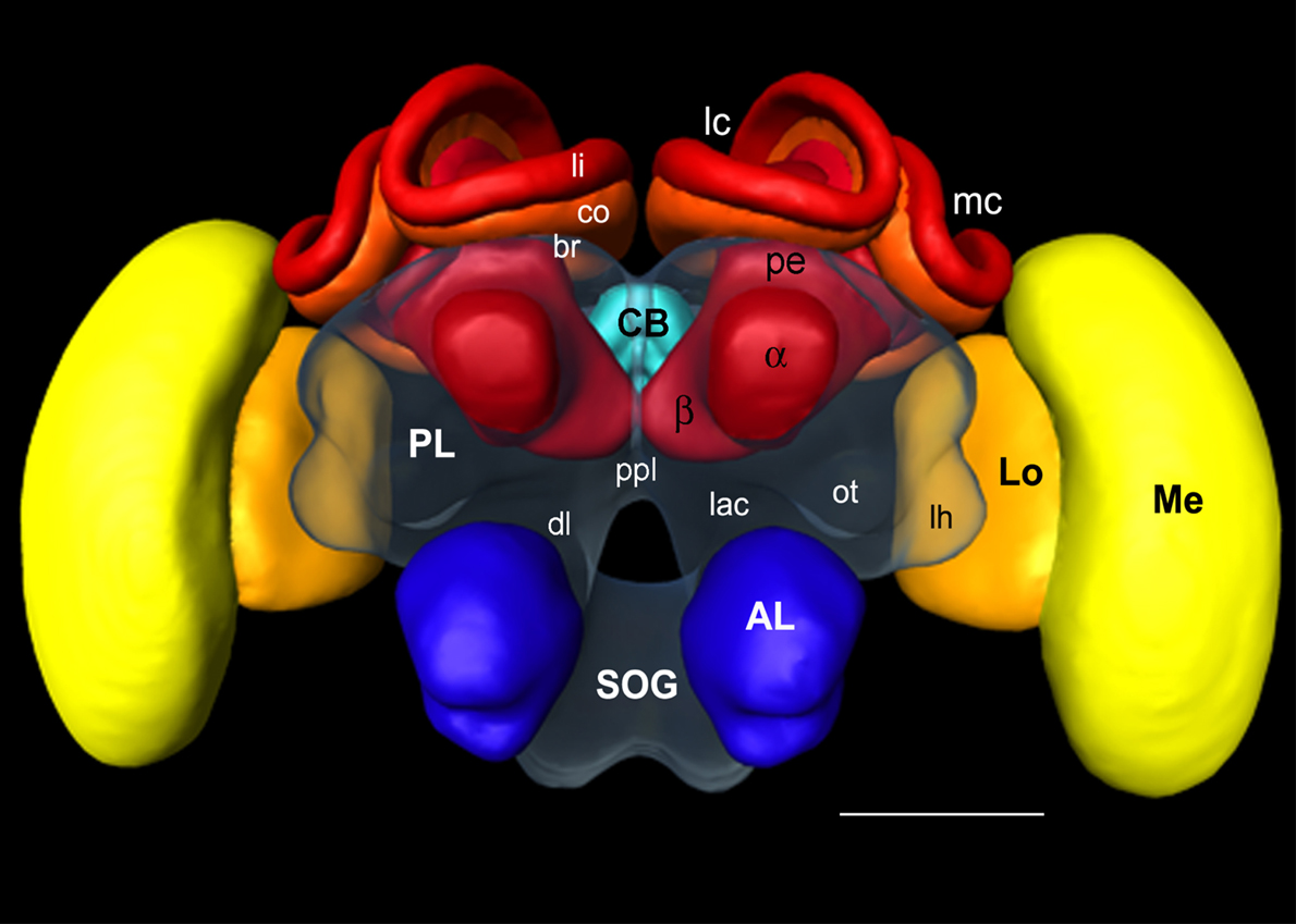
Figure 1. Surface reconstruction of the honeybee standard brain (HSB). Neuropil areas defined in the HSB are shown in different colors. Components of the midbrain area (protocerebral lobes, PL, and subesophageal ganglion, SOG) are fused and shown in transparency. Subcompartments of the protocerebral lobe and mushroom bodies are indicated in lower case letters. Scale: 300 μm. PL: protocerebral lobe; ppl: posterior protocerebral lobe, Lo: lobula; Me: medulla, li: lip, co: collar, br: basal ring, lh: lateral horn, ot: optic tubercle, lac: lateral accessory lobe, mc: median calyx, lc: lateral calyx, pe: peduncle, α: alpha-lobe, β: beta-lobe, SOG: suboesophageal ganglion.

In Figure 2 several examples of neurons are shown, each stemming from a different preparation, and each having been separately transformed into the HSB. To capture all parts of a neuron at different resolutions, several confocal scans were necessary. This poses the problem of registering several label fields leading to subsequent errors during realignment of all parts of the neuron that accumulate during the registration processes, which may induce artifacts at the edges of the label fields (Maye et al., 2006). The strategy used for each of the examples of Figure 2 was to first scan an overview of the brain containing the whole neuron, and then reconstruct the main parts of the neuron. Afterwards, the neuron’s regions of interest, for example, the dendritic tree of the L3 neuron, were reconstructed from high-resolution scans (Figure 2B), downscaled, aligned, and merged to the main neuron reconstructed from low resolution scans. Deviations that are caused by using several independent regions of the same neuron in several steps of registration are kept to a minimum. As a result, the spatial accuracy of the warping process is enhanced. This iterative procedure allows us to compose compounds of registrations at different levels of resolution, for example, the target areas of olfactory and mechanosensory interneurons (Ai et al., 2009) in subregions of the protocerebral lobe (arrows in Figure 2A) together with registrations at high resolution of their fine structures for the analysis of their local topological features (Figures 2C,D). The movie of supplementary material S3 and the interactive viewing mode in the PDF file (Figure 2A) allows visualization of the neurons’ spatial relationships.

FIGURE 2

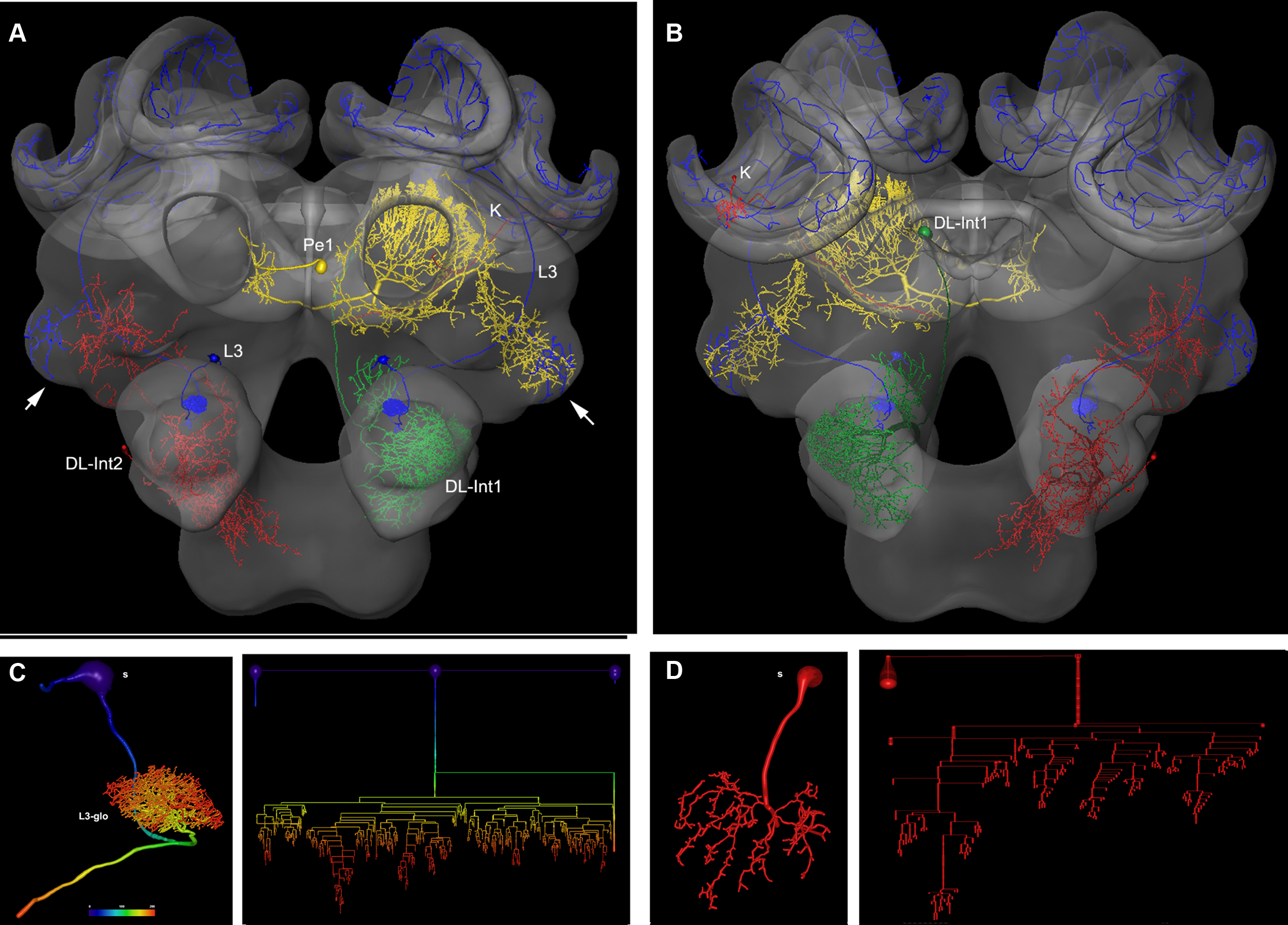
Figure 2. Olfactory (L3: blue) mechanosensory (dorsal lobe interneuron 1 and 2: DL_Int1, green, DL_Int2, red) and central interneurons (Pe1, yellow) registered into HSB. A mirror image is exhibited for the L3. (A) frontal view (B) caudal view. The projection areas in the lateral protocerebral lobe are compared (arrows). They occupy either separate neuropil areas: L3 and DL_Int2, or L3 and Pe1 overlap. (A) The L3 neuron projects to the lateral horn (arrows) and mushroom body calyces (MC, LC). The axonal terminals of the L3 neuron form microdomains in the lip region of the calyces and overlap with the dendritic fields of Kenyon cells (K, in B). Scale: 50 μm. (C, D) Neuron reconstruction and dendrogram of the respective neurons derived from high-resolution confocal scans. In (C) the neuronal distance is indicated in color. See false-color coded bar. (see also movies of supplementary material S3).

Estimating the accuracy of the registration process is a difficult task. Certainly, the process involves numerous steps, which are prone to induce inaccuracies (see above). For example, the histological procedure may induce variable distortions due to local shrinkage differences that are not fully compensated by the affine and elastic registration. The experimenter may not segment correctly; the number of label fields (and, thus, the number of registrations steps) and thus distortions of the reconstructed surfaces of neuropils and neurons will lead to incorrect locations of the transformed neuron in the HSB. In addition, the neuropils and neurons themselves will differ from animal to animal, and it is this variability that determines the fundamental limit regarding the reliability of any brain atlas – besides the methodological problems. Therefore, it is not possible to derive a measure of reliability in the composition of neurons registered sequentially into the brain atlas. The best way of checking the spatial accuracy of such neurons is by comparing the relative positions of the neuron to the neuropil border lines in the original preparation to the situation after the registration process. We provide circumstantial evidence for the reliability of the segmentation and registration process by describing an example in which we compared the locations of intracellularly stained neurons with cross sections in high- resolution ethyl gallate-stained paraffin sections using two different registration methods.

Integrating Data Collected by Different Histological Methods

In Figure 3 a registered olfactory projection neuron (L5) is visualized together with a registered ethyl gallate section showing midbrain regions (mushroom bodies, central body, and protocerebral lobe). The ethyl gallate method (Wigglesworth, 1957) provides detailed information about the neural architecture revealing the composition of neuropils, somata, and tracts, thus capturing the spatial context information. A whole series of ethyl gallate-stained sections was first used to identify the median and lateral antenno-cerebralis tracts (ACTs) in a correlative light and electron microscopy study (Rybak, 1994). Our future goal is to integrate data from these histological procedures into the HSB. Here, we demonstrate the spatial accuracy of the registration process. A horizontal ethyl gallate section was warped into the HSB using a landmark-based registration by finding corresponding points or landmarks in the HSB and the histology section (Figure 3). Separately, a single stained L3 axon, which was transformed to the HSB using a label field registration, runs through the corresponding ascending and descending parts of the median ACT (m-ACT) as seen in the ethyl gallate section (Figures 3A–C). The spatial accuracy of the registration process is indeed very high, and allows identification of m-ACT neurons in the median and lateral antenno-cerebralis tract (l-ACT) even at the single neuron level (see black arrows in Figure 3B).

FIGURE 3

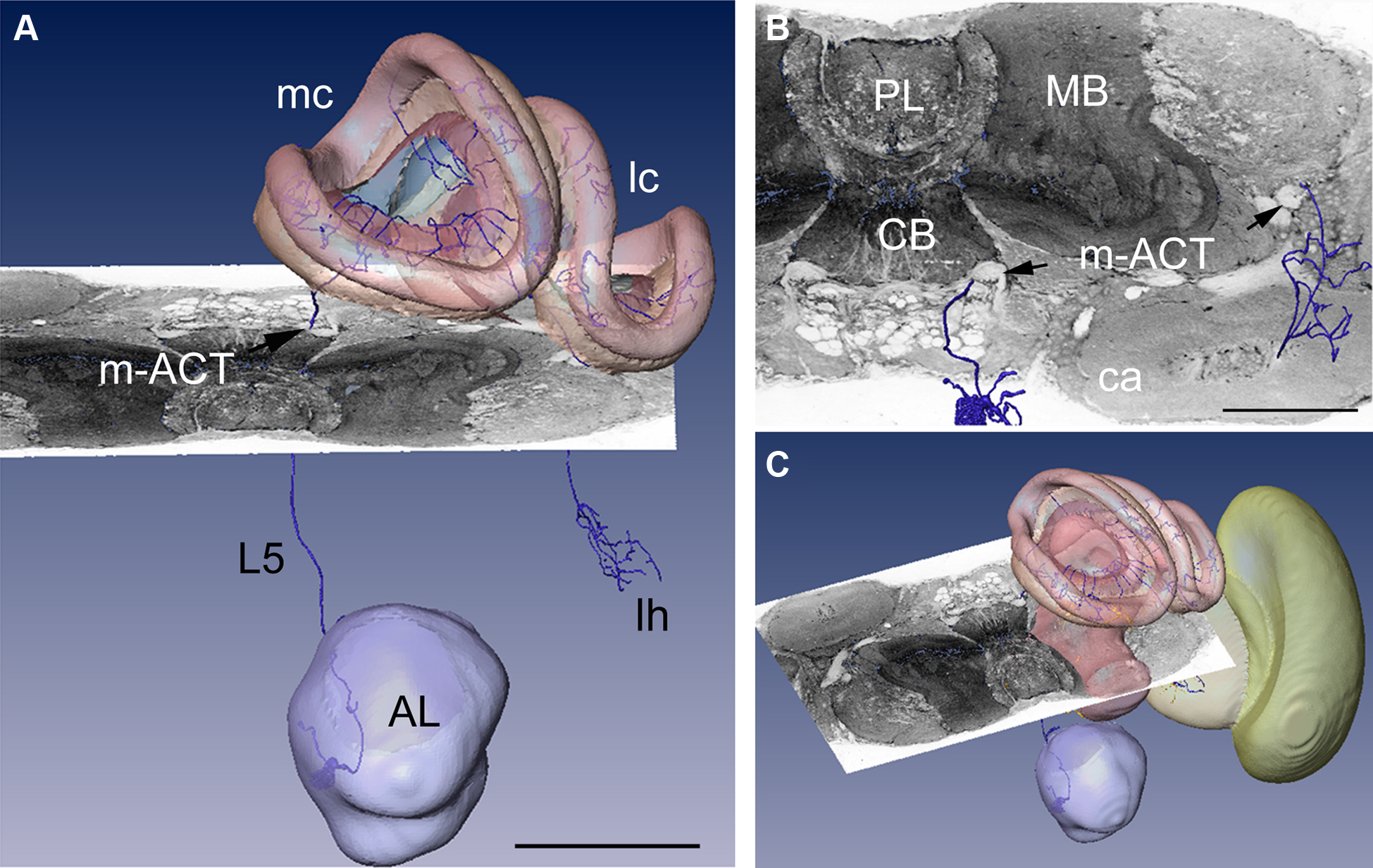
Figure 3. Visualization of the neural architecture of the midbrain from two different preparations using landmark and label field registration techniques. (A) The L5 projection neuron (in blue) of the median antenno-cerebralis tract (m-ACT) connects the antennal lobe with the mushroom body calyx (MC, LC) and lateral horn (LH), L5 axon (black arrow). (B) The m-ACT can be identified in a cross section as the ascending and descending protocerebral part (m-ACT, black arrows). The spatial locations of the two registrations demonstrate the spatial accuracy of fitting neuronal data into the HSB. (C) The histological ethyl gallate section is located at around 300 μm from the calycal surface (horizontal plane). Scale: 200 μm, CB: central body, MB: mushroom body, PL: protocerebral lobe.

Analyzing Putative Synaptic Connections

Fitting neurons into the HSB can be achieved with a certain degree of accuracy with regard to spatial relationships, but thus far cannot replace studies on synaptic connectivity. This must be achieved by electron microscopy (e.g., Ganeshina and Menzel, 2001) or by some approximation in confocal co-localization studies on the light microscopy level. Combining high-resolution confocal laser scanning microscopy with precise three-dimensional dendritic surface reconstruction (Schmitt et al., 2004) allows for automated co-localization analysis in order to map the distribution of potential synaptic contacts onto dendritic trees or axon terminals (Evers et al., 2005; Meseke et al., 2009).

This technique was used to estimate the distribution of putative GABAergic synaptic contacts on the dendrites of the Pe1 neuron, a single identified mushroom body extrinsic neuron (Mauelshagen, 1993; Rybak and Menzel, 1998, Figure 4). GABA-like immunoreactivity has been shown for the A3 feedback neurons (Schäfer and Bicker, 1986; Grünewald, 1999). These neurons also innervate the mushroom body lobes and peduncle and may provide local inhibitory input to the Pe1 neuron (Figure 4B, green label). In Figure 4D the distribution of putative inhibitory input synapses onto the Pe1 dendritic tree is highlighted by red dots, indicating a distance of GABA-like immunoreactivity profiles of up to about 300 nm (Okada et al., 2007).

FIGURE 4

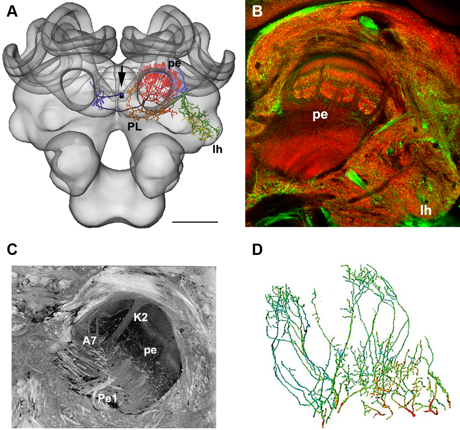
Figure 4. (A) The Pe1 neuron fitted into the HSB (skeleton view). Different parts of the neuron are colored according to their innervation of subneuropils in the central bee brain. (B) GABA-IR in the bee brain. Double labeling of GABA-IR-like (green) and synapsin staining (synorf1, red). The optical section cuts the mushroom body at the transition zone between the α-lobe and peduncle (pe), lh: lateral horn of the protocerebral lobe. (C) A histological section of the central bee brain stained with ethyl gallate reveals the neural architecture of the mushroom bodies at the transition from the α-lobe to the peduncle. The large axon diameter of the Pe1 is identified as a single unique neuron. A7: type 7 α-lobe extrinsic neuron, K2: strand of Kenyon cells type 2, PE: peduncle. (D) The finger-like dendritic protrusions of an intracellularly marked and reconstructed PE1 neuron branch all over the cross section of the mushroom body at the border line between the β-lobe and the peduncle. These branches are organized in two regions (the proximal domain 1 and the distal domain 2) where the Pe1 is postsynaptic. Red dots indicate close appositions of GABA-IR profiles (arrows), which are more numerous in domain 1. Scale bars: (A) 200 μm.

To achieve the accuracy required for neuronal connectivity estimates, the development of higher resolution atlases that define subregions of the brain and allow their integration into a common coordinate system is needed. An example is given in this special issue of Frontiers in Neuroscience by el Jundi et al. (2010) who constructed a high-resolution atlas of the central complex of Locusta and determined the spatial relations of two central complex neurons.

The Statistical Shape Model (SSM)

Advantage of the SSM

The accurate and reliable localization of region boundaries during the registration process is a prerequisite for fitting neurons into any Standard Atlas. This is true for manual (or semi-automatic) and fully automatic segmentation techniques, though the advantage of the latter is that the level of human expert interaction is reduced. Labeling performed by different individuals often leads to variable results. A model-based auto-segmentation of neuropil boundaries utilizes a priori knowledge about the 3D shape of an object, in our case the bee brain, and characteristic features of the imaging data. Such a model provides a measure of the variability of the object set and can therefore be used to analyze and quantify morphological volumetric changes in neuropiles of the adult animal.

An SSM of the central bee brain (excluding the antennal and optic lobes) was calculated from 16 training shapes, resulting in 17 shape modes. These were extended to 32 shapes (31 shape modes) by mirroring the right and left brain hemisphere along the neuraxis in each preparation. Each training shape was manually segmented by labeling the neuropil boundaries of the confocal imaging data stained with Lucifer yellow. Triangulated polygonal surfaces were reconstructed from the labeled images and simplified to 150000 triangles. The surfaces were then affinely aligned using the geometrical center as a reference point, and then transferred to a common coordinate system. In order to map the surfaces of the training shape in a proper way, certain conditions are required for creating the surfaces (for details see Lienhard, 2008). In order to achieve a correct model of a biological structure, one needs to find the corresponding anatomical points on all training shapes. To determine correspondences, surfaces were divided into 89 regions according to shape features and anatomical landmarks (Figure 5A). A principal component analysis provided a linear model of the shape variability of the training set (Figure 5B, see also the Movie in section "The statistical shape model" of supplementary material).

FIGURE 5

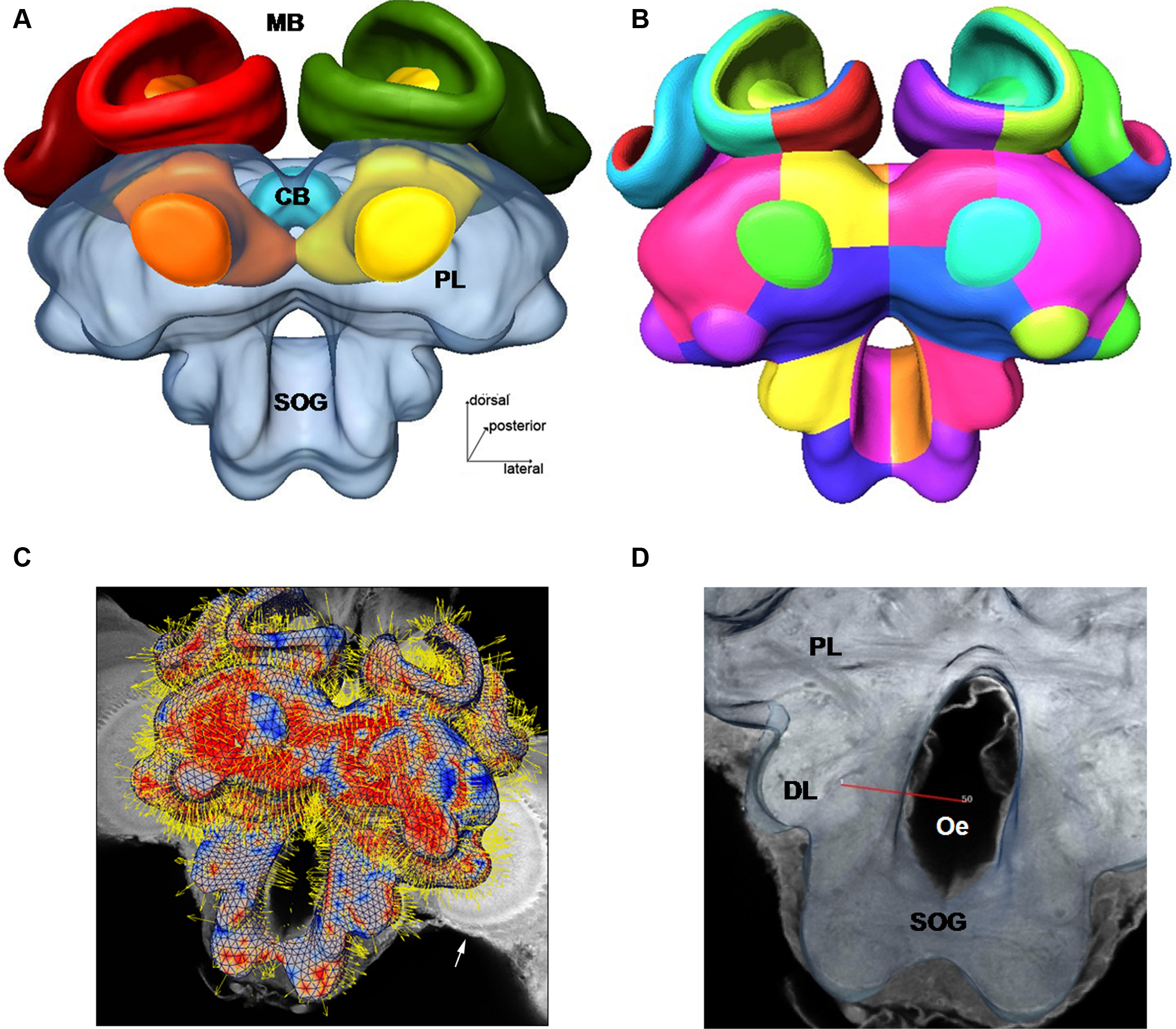
Figure 5. (A) The surface of the statistical shape model (SSM) of the central honeybee brain (with exception of the antennal and optic lobes) derived from 16 segmented worker bee brains. The calyx regions of the mushroom bodies are not subdivided. (B) Patch decomposition: in order to find correspondence among the set of training data the surface of each segmented brain is subdivided into 89 patches (colored regions). (C) Position of the displacement of the bee brain model in the imaging data. Displacement vectors are shown as yellow arrows, blue color indicates the displacement vectors point outwards, red means they point inwards. The white arrow indicates one orthogonal slice of the 3D confocal image stack to which the model adapts. (D) A protocerebral region close to the esophagus is shown to demonstrate matching of the SSM (in transparency) to the corresponding gray-value confocal image. The red line marks the intensity profile (length 100 μm) along the vertex normals (adapted from Lienhard, 2008; Singer, 2008) for (A): see also S4 movie in supplementary material.

In order to place the SSM of the central bee brain roughly into the confocal images an affine registration was used applying a non-deformable model that contained only brain regions that represent borders to exterior structures. A positioning algorithm recomputed rotation, scaling, and translation parameters using characteristic image features of brain tissues. In order to reduce noise in the low-contrast Lucifer yellow stain a non-linear isotropic filter was applied to the data (Weickert, 1997; Lamecker et al., 2004).

The SSM-based segmentation algorithm, as described in the section “Methods”, was applied until no further improvement could be achieved, meaning that the change of the shape between consecutive iterations fell under a defined threshold. The displacement vectors were computed via analyzing 1D profiles of image intensities along surface normals at each vertex (Figure 5D). Based on these displacements the SSM was iteratively adapted (see Figures 5C,D and the movie in section "Automatic segmentation" of supplementary material). The process of initial positioning and the adjustment of the model in an exemplary training dataset image (LY12) are shown in Figure 6.

FIGURE 6

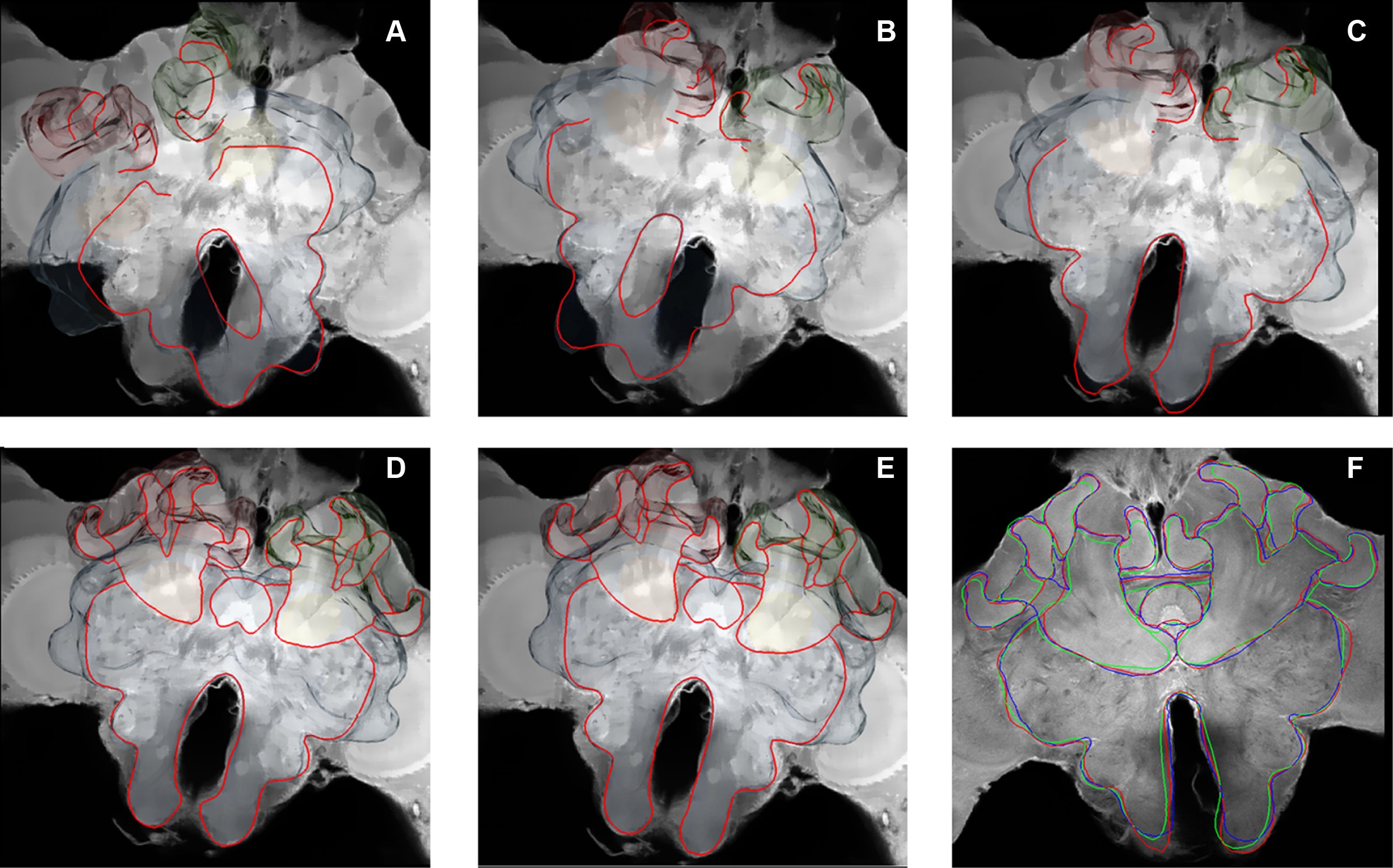
Figure 6. Evaluation of the statistical shape model (SSM) and the displacement algorithm. The auto-segmentation process illustrated by a leave-all-in segmentation of preparation LY-12 (Lucifer yellow background stain) with the SSM. (A) Initial position of the average shape of the lateral mushroom body. (B, C) Result of the initial global positioning of a simplified SSM (which consists of just one individual surface). (D–F) Result of the optimization of the position and shape parameters in red. The result of the original manual segmentation is shown in blue. The result of the automatic segmentation process using a leave-one-out test is shown in green. (From Singer, 2008). See also S5 movie in supplementary material.

Application of the segmentation algorithm on the training set images results in an average surface distance of 4.06 ± 0.95 μm of the fitted model to the manual segmented shapes. A leave-one-out test simulating new image data yields to a distance of 8.82 ± 1.02 μm. In comparison, two manual segmentations of the same imaging data lead to a mean surface distance of 4.79 μm.

The SSM and displacement algorithm was also tested with confocal data not contained in the training set that was used for creation of the shape model. We used extracted parts of the SSM in combination with the displacement model in order to automatically segment the mushroom body neuropil in high-resolution confocal scans (Figure 7A). Figure 7B shows the results for a single section using either the whole mushroom body calyces (red intersects) or the calyces (yellow intersects) to auto-segment the structures. Slightly better results were achieved using the reduced model of the calyx (arrows in Figure 7B). Figures 7C,D shows manually segmented neuropil borders in comparison to the automatic segmentation. Figure 8 provides a direct comparison of the HSB and SSM. The mean surface distance between HSB and SSM amounts to 8.5 μm. Particularly large distances were found at the median calyx (MC) and subesophageal ganglion (SOG), possibly indicating stronger shrinkage dependencies induced by the different histological procedures. It takes an experienced segmentor around 8 h to manually segment those central brain structures used for the SSM.

FIGURE 7

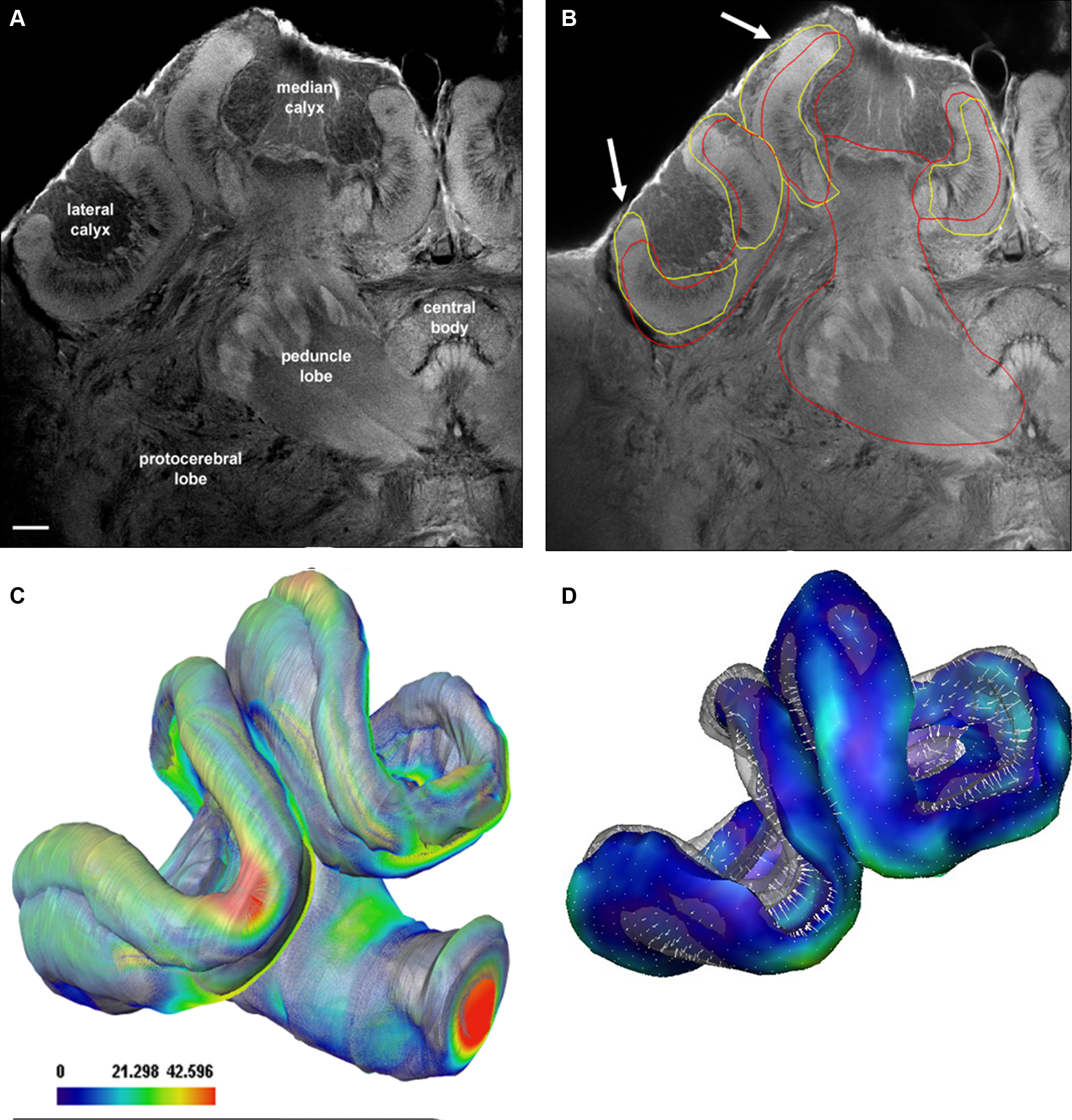
Figure 7. Evaluation of the auto-segmentation process using a reduced shape model for confocal imaging data. (A) Confocal Lucifer yellow image of the median and left brain hemisphere scanned with a 20× oil objective. (B) Result of the automatic segmentation process. Arrows indicate refinement of automatic segmentation using isolated neuropils: yellow lines when only the calyx was used, red line when the whole mushroom bodies were used. (C, D) Surface representations of shape differences between manually (transparent) and automatically segmented (solid) labels. The mean surface distance of the manually segmented and the automatically segmented surface is 11 μm using the mushroom body model of the SSM as compared to 10.5 μm using the calyx model. Scale bar in (C): surface distance in μm.

FIGURE 8

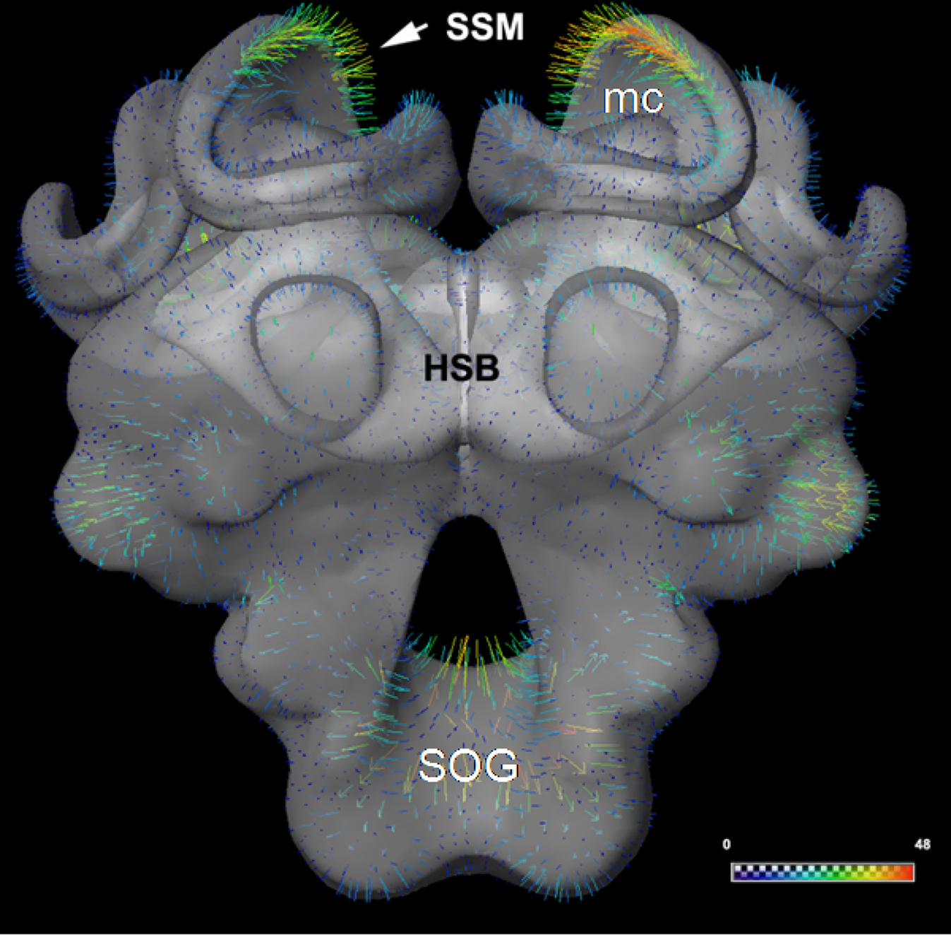
Figure 8. A comparison of the iterative average shape brain (HSB) and the statistical shape model (SSM). The mean surface distance measured after rigid registration of HSB onto the SSM amounts to 8.5 μm. Only the surface model of the HSB is shown here, and the surface distances between HSB and SSM are indicated by colored vectors (arrow and false-color scale bar). Note the particularly large distance at the median calyx (MC) and subesophageal ganglion (SOG), which might be due to the stronger shrinkage process caused by the different histological procedures employed for the two models (see section “Methods” and text).

In contrast, a further evaluation of the quality of automatic segmented bee brains and the estimated post-processing times amounts currently to approximately 3–4 h by an experienced segmenter.

Hierarchical Structure Labeling and Browsing

The HSB created so far contains only geometric and topological information about neurons and neuropils. For many applications, semantic information also needs to be integrated. This semantic information includes information about the hierarchical organization of brain structures and information about relations between structures. An example would be the description of the anatomical proximity of neuron A and neuron B and the possible communication between them. Often neurobiologists have this knowledge, but the information needs to be made explicit.

In recent years, the development of ontologies has been an appropriate choice for capturing and representing semantic information in many fields, including biology. In the information sciences, an ontology is a formal representation of concepts or structures and relations among those structures in a defined application domain. Visually, ontologies can be described as graphs in which structures are represented by nodes and relationships between structures by edges. In ontology modeling, there are two different types of nodes: classes and instances. Classes describe common concepts, such as brain. An instance of such a class could be, for example, the brain of animal A. Relations appear among classes, among instances, and among classes and instances. Relations can have different types, as for example the type isA. With these basic tools we can create the statement brain of animal A isA brain.

To support the understanding and analysis of structural and functional characteristics of brain structures, ontologies need to fulfill several requirements. An ideal brain ontology would include a complete set of structural parts and neuron types. It would also contain axonal projections between regions and neuron types, and it would include morphological, connectional, and functional properties of these particular neurons. According to Bota and Swanson (2008), an ideal ontology would be species specific. These authors also state that the development of such an ontology is a long-term goal for a community project. Indeed, we consider our attempts as an early step only.

Our ontology uses predefined classes of the foundational model of anatomy (FMA) (Rosse and Mejino, 2003). The most important of these are Cell, Cell_Part, Organ, and Organ_Part where Cell and Cell_Part only consider neurons and Organ and Organ_Part only consider neuropils of the bee brain. We further restrict our relations to describe spatial, morphological and, if available, connectional properties. Table 1 lists the most important relations used in our bee brain ontology. Figure 9 shows a scheme of how classes, instances and relations are connected using the Pe1 neuron as an example (see also Figures 2 and 4). The editor Protégé was used to create the ontology. Currently, the ontology contains 100 classes attached to 600 instances, and 1300 relations of 17 types. Integrated are several neuron types including the location representation of their somata, axons, and dendrites. This ontology has been linked to the reconstructions of the HSB by assigning the reconstructions’ ID and file name to appropriate instances of the ontology. This step enables ontology-based browsing of the atlas (Kuß et al., 2008, 2009).

TABLE 1

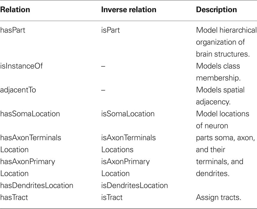
Table 1. The most important relations used in our bee brain ontology to describe spatial, morphological and, connectional properties.

FIGURE 9

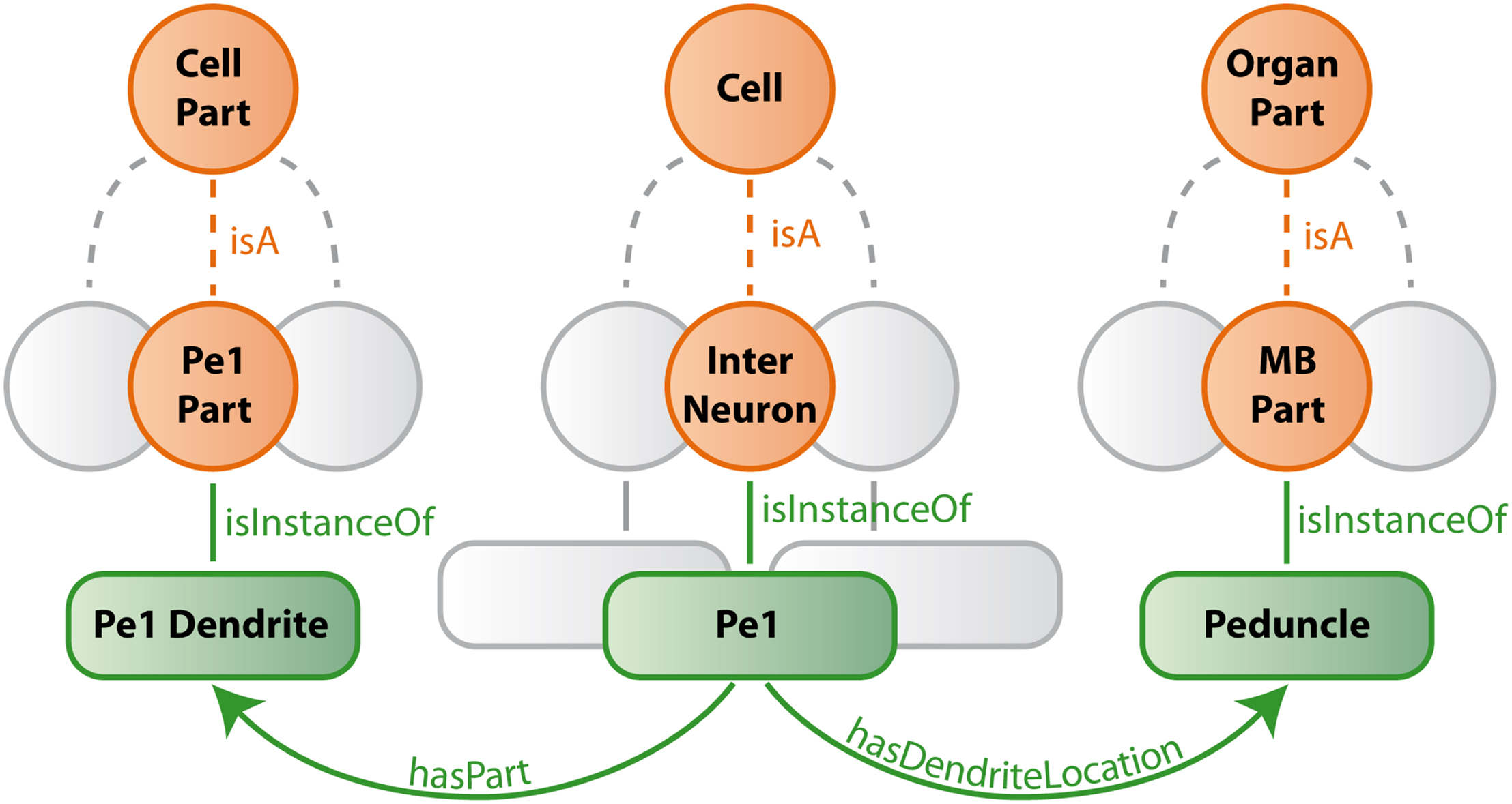
Figure 9. Schematic description of bee brain ontology (with the Pe1 neuron as an example). Orange circles symbolize classes which represent summarizing concepts of structures with similar properties. Green rounded squares symbolize instances of classes which are connected by green edges (relations) to each other. Gray structures indicate that only a small selection is presented.

In a first usage approach of the ontology-linked HSB, we addressed the automatic creation of meaningful visualizations. Good visualizations transport a large amount of information and form an important communication medium. This information can be used to present research results, to communicate with research partners or to teach neurobiology. Often the process of creating such meaningful and expressive visualizations is time-consuming and requires sound knowledge of the visualization software used. In our approach, the user only selects a structure to be visualized and a predefined query, such as “Show overview”. Then, an algorithm automatically creates a visualization that contains the selected structure highlighted as a focus object and further structures forming the context. This works as follows: Each predefined query owns a set of relation types considered to be relevant. Starting at the selection, the algorithm then looks within the ontology for other structures in the vicinity of the selection that may be of interest for the desired visualization. Only structures connected via a relation type relevant to the query are of interest.

Discussion

The motivation for creating a digital atlas of the bee brain originated from the experience that a large amount of information is lost when single, intracellularly marked neurons are drawn on paper traced in camera lucida projections or just photographed. Neurons are three-dimensional entities embedded in a network of other neurons, and it is this information that is required in the future to interpret functional properties of neurons and neural networks in relation to their structure and connectivity (Abel et al., 2001; Müller et al., 2002; Krofczik et al., 2008). Insect brains are small enough to be scanned fully with confocal microscopy at a reasonable resolution. Therefore, no border problem appears, or at least it is reduced to the spatially limited connections with the ventral chord. Furthermore, many neurons in the insect brain are individually identifiable, and quite a number of them have already been identified (e.g. Hammer, 1993; Mauelshagen, 1993; Menzel, 2001; Heinze and Homberg, 2008; Homberg, 2008; see also this issue). Often neural tracts or compositions of local neurons consist of a few hundred neurons allowing for the possibility that in the not too distant future all neurons of a particular neuropil or part of the brain will be described in their morphology. In that case one would need this “description” in a digital 3D format so that the full power of mass data computation can be applied to visualize zoom determine potential connectivity patterns, to derive quantitative measures of distances, diameters, branching patterns, potential synaptic sites, and relate structures to functional components such as distribution of transmitters, receptors, channels, and intracellular molecules. At the moment we are far from getting even close to these goals, but important groundwork has been done, and one can hope that the time- consuming (and tedious) steps towards reaching these goals, such as manual segmentation, correction of errors, complicated procedures during registration, neuron tracing, (see Maye et al., 2006) will soon be overcome or become less cumbersome (for an review on automated registration and neuron tracing methods, see Peng, 2008). Apart from the aesthetic pleasure one experiences in visualizing single neurons and their compositions within the 3D atlas, right now the reward gained from creating the brain atlas and filling it with useful information is limited to understanding the spatial relationship. But this will soon change, because the information stored in the framework of the atlas will allow us to pose new questions, to discover novel patterns of neural connections, to assemble and organize large amounts of information, and to relate function to structure as proposed by us as well as other authors (e.g. Namiki and Kanzaki, 2008; Staudacher et al., 2009).

We began our project by creating an average atlas from 20 bee brains whose 22 neuropils were segmented manually and then used for the averaging process. The composition of these neuropils made it possible to calculate rigid and elastic transformations that provided enough information for faithful registration of neurons. The average-shape property ensures that the deformation applied to the individuals remains small. Furthermore, manual segmentation as applied in our first approach is subject to noise, i.e., contouring between slices varies according to criterion variability of the experimenter. Averaging several such noisy label images reduces random parts of the contours, thus increasing the reliability of the standard. We have shown (Rohlfing et al., 2001; Brandt et al., 2005) that the non-rigid registration is able to increase the distinctness of inner structures such as tracts and strata even though the algorithm does not “know” about those structures, because it is applied on the label images without interior structures. We deduced from our observations that registration fidelity is sufficient for the spatial scale level of the standard brain. This result also makes us optimistic that a non-rigid registration of neuropil boundaries to the standard yields a reliable and reasonably accurate estimate of the “true” position of a co-stained neuron within the standard.

As pointed out above, it is not easy to evaluate how accurate the registrations of neurons are using the average neuropil borders as guiding posts. When a neuron runs close to the border of a neuropil used for registration a small deviation from its relative position becomes very important, that is the neuron lies either inside or outside the particular neuropil. We have observed these inaccuracies, and they can be corrected by repeating the segmentation and registration processes (see section "Registration protocol" of supplementary material). Preparation artifacts due to dissecting of the specimen and histological processing can lead to distortion effects that are only partly corrected by the registration algorithm. Further inaccuracies are due to surface reconstruction (smoothing) from segmented label fields, and to cropping of areas of interest. For the latter the edges of cut regions are not well defined for the individual brain and the standard reference and are therefore difficult to operate for the registration algorithm (Maye et al., 2006).

The question of whether two close neurons are potentially in synaptic contact is much more difficult to answer and may well be beyond the scope of the registration process. Double markings in the same brain combined with electron microscopy will also be necessary in the future to prove such contacts, but the registration process already provides conclusive evidence that will either provide the motivation to start such a demanding project or forsake it altogether (e.g., Hohensee et al., 2008; Meseke et al., 2009). We provided one example to document that registered neurons are so precisely embedded in the histology of high-resolution light microscopy cross sections (Figure 3) that one may well conclude that their location relative to surrounding neurons is down to the precision of a few microns. In a similar approach single-cell labeling was used in combination with non-rigid registration techniques to estimate the synaptic density and spatial relationship of Drosophila olfactory interneurons (projection neurons) in central brain areas (Jefferis, 2007). Using intensity-based image registration for averaging the brains, they estimated the accuracy of registration up to a few microns. Greater accuracy might not be possible because the protocols always depend on neurons from different brains, and the variance of neuron Gestalt from brain to brain will limit the resolution.

A general problem with neuron reconstructions relates to the fact that high-resolution imaging microscopy requires lenses whose working distance is often not large enough to cover the whole dendritic tree of the respective neuron, whereas low resolution images are necessary to connect parts of the same neuron or different neurons. Physical sections, e.g., vibrotome offer a solution to this problem, but consecutive sections need to be aligned such that the neuron can be fully reconstructed and registered into the atlas (el Jundi et al., 2009, 2010).

So far we have registered 50 neurons into the HSB, a small proportion indeed of the approximately 950000 neurons of the bee brain (Witthöft, 1967). However, even this small number calls for more sophisticated means of visualization, selection of combinations of neurons and ways of highlighting particular properties of the network arising from these neurons (potential contacts, estimated information flow, combination with data from, for example, immunocytochemistry and electron microscopy, electrophysiology, and Ca-imaging).

The Statistical Shape Atlas

An atlas derived from an averaging process (as the HSB, Figure 1) contains a large amount of information about spatial relations of structures. It is highly suggestive to use this information for one of the most time-consuming, difficult and tedious steps, the segmentation process of the structures (neuropils) necessary for the registration of any individual brain. We took up this argument and implemented a procedure, a model-based auto-segmentation, originally developed for the analysis of shape variability and modeling of structures in medical imaging (Lamecker, 2008). This method was adapted and applied to the central bee brain to generate a SSM (Figure 5) that reflects the shape variability of a restricted set of 16 bee brains. In combination with a displacement model (Kainmüller et al., 2007, 2009; Lamecker, 2008), based on evaluation of intensity gradients within the confocal images, the SSM allows automatic neuropil segmentation (Figures 5–7). Our approach was combined with alterations in the histological procedure. Lucifer yellow was used instead of synaptic antibodies as a neuropil background stain. Furthermore, only a selected part of the brain was used (the central brain excluding the antennal lobes). Lucifer yellow treatment during the histological procedure provides us with the same information as the antibody, but is faster and the results in more homogenously stained neuropils. The focus on the central brain allowed us to test the power of the approach for the most important and most complex structures of the bee brain, the mushroom bodies (Figures 4 and 7). An automatic procedure for segmenting neuropils provides the following additional advantages: (1). A priori knowledge about the 3D shape of the objects in question, in our case, the bee brain with its characteristic features of the image data. (2). Measures about the variability of the object set, and thus provides us with information which can be used to analyze and quantify any changes induced during development or on the basis of different genetic backgrounds (as described by Kurylas et al.,, 2008; el Jundi et al., 2010 for the VIB). (3). Information useful for across-species investigations in order to analyze evolutionary changes by comparative analysis of brain structures at least in closely related groups (e.g., hymenoptera, Gronenberg, 2001; beewolf, Rybak et al., 2003).

We found that SSM can well be used to detect neuropil borders in these preparations. Nevertheless there are deviations in the automatic segmentation process (see Figure 7). An analysis of the post-processing time by a segmentation expert shows that one still saves considerable time and gains accuracy (Rybak, personal observation).

A quantitative comparison of HSB and SSM (Figure 8) reveals that the volume of the HSB is smaller relative to the SSM. Stronger shrinkage of the HSB might be due to the prolonged incubation time required for the synaptic antibody procedure (1 week). Nevertheless, since shape differences in segmented brains by either the synaptic antibodies or the Lucifer yellow method seem to be small, it is reasonable to take segmented data used for the HSB and include it into the enlarged model of the SSM. Moreover, all imaging data used for the HSB were segmented by experts, thus providing very reliable definitions of the neuropil boundaries, and the quality of the SSM will be enhanced by adding the HSB dataset, since shape variability represented by the enlarged SSM will capture a higher number of histological procedures used for insect preparations (i.e., fixation, incubation of antibodies, use of fluorescent dyes).

One disadvantage of the current HSB is that it is closed to improvements and adaptations, which will certainly result from more appropriate histological procedures such as the shift from antibody staining of neuropil borders to easy-to-use fluorescent dyes. Working with the SSM will allow us to create a novel form of HSB that grows with each brain, and which adapts stepwise any morphological changes with histological procedures. Thus, enlarging the set of brains included in the SSM by already segmented brains used for the HSB and by developing more elaborated displacement algorithms based on intensity profile analysis will allow us to create such a new atlas based on many more brains, particularly in the context of different experiments (electrophysiology, immunocytochemistry, etc). Additionally, combining a shape atlas with proper registration techniques will allow us to use such an atlas, initially created to replace manual segmentation (for the label field registration of neurons). Once the deformation field that fits the SSM model to a confocal image is calculated it can be used to integrate the neuron into the average-shape atlas. Such an approach can forego and eventually replace the label field registration as in the current HSB.

Conflict of Interest Statement

The authors declare that the research was conducted in the absence of any commercial or financial relationships that could be construed as a potential conflict of interest.

Acknowledgments

We thank Alvar Prönneke for his help in evaluating the SSM Vincent Dercksen for landmark registration and Dirk Drenske for help with the 3D-PDF. We are particularly grateful to Gisela Manz and Astrid Klawitter for help with the reconstructions. We would also like to thank Daniel Münch and Hiro Ai for providing data for Figures 2 and 4.

Note

An Interactive three-dimensional view of the Honeybee Standard Brain and integrated neurons for Figures 1,2A and 4A can be found in the 3D PDF file in the supplementary section. In order to utilises the 3D tools requires viewing with Adobe Acrobat Reader 8.0 or greater.

Glossary

Labelfield There are two ways to represent segmentations of images: either boundaries are added to an image that enclose sets of pixels that are considered to belong together, or to pixels/voxels a label (a specific ID) is assigned that represents a particular object. In Amira the label field representation is used.

Ontology In the information sciences, an ontology is a formal representation of concepts or structures and relations among those structures in a defined application domain. They represent semantic information using a controlled vocabulary. Visually, ontologies can be described as graphs in which structures are presented by nodes and relationships between structures are represented by edges.

Registration The process of computing a coordinate transformation that maps the coordinates of one image onto the anatomically equivalent point in another image.

Segmentation Classification of regions (intensity values) within the image data and partition of homogenous regions. The use of a single threshold means binarization of the image, i.e., separation of background and structure of interest. Segmentation may separate many structures within the image (connected components or segments of the image).

Transformation Mathematical operation that moves, rotates, scales, and/or even deforms an object in such a way, that it will be aligned to another similar one.

Warping Reformatting of an image under a deformation given by a non-rigid coordinate transformation. This is also known as also elastic or free-form deformation.

Glossary on the Internet: http://en.wikipedia.org/wiki/ Image_ registration.

http://life.bio.sunysb.edu/morph/glossary/gloss1.html.

http://life.bio.sunysb.edu/morph/glossary/gloss2.html.

Supplementary Material

The Supplementary Material for this article can be found online at http://www.frontiersin.org/systemsneuroscience/paper/10.3389/fnsys.2010.00030/

Supplement 1: Colorwash HSB  movies in wmv format

These movies show confocal images of the honeybee brain in frontal, horizontal and sagittal directions. Neuropils were stained with synaptic antibodies. The colored label fields of brain neuropils as defined for the Honey Bee Standard Brain (HSB, Brandt et al., 2005) are superimposed. Note that some neuropil areas that are not defined in the HSB are labeled. Abbreviations: AL: antennal lobe, a: alpha-lobe, b: beta-lobe, CB: central body, li: lip, co: collar, br: basal ring, Me: medulla, Lo: lobula, PL: protocerebral lobe, SOG: subesophageal ganglion. MC: median calyx, LC: lateral calyx. ot: optic tubercle,, pb: protocerebral bridge, DL: dorsal lobe, lac: lateral accessory lobe, pe: peduncle, lh: lateral horn.

Supplement 2  pdf

Registration Protocol that describes the incorporation of neuronal morphologies into the Honeybee Standard brain (HSB).

Supplement 3  movies in mpg format

a The spatial relationship of olfactory L3 neuron (blue), mechanosensory (DL and 2: green and red, respectively) and central interneuron Pe1 (yellow) after transformation to the Honeybee Standard Brain (HSB).

b the same movie in stereo mode

Supplement 4  movie in wmv format

The Statistical Shape Model: Visualization of the central brain and morphological variations of the mushroom bodies and protocerebral neuropils (for more details: see text and Lienhard, 2008).

Supplement 5  movie in wmv format

Displacement model: Positioning and Displacement of the central brain model in the image data. Reddish-white flickering indicates the deformation of the model during the adjustment of the SSM to the image data.

References

Abel, R., Rybak, J., and Menzel, R. (2001). Structure and response patterns of olfactory interneurons in the honeybee, Apis mellifera. J. Comp. Neurol. 437, 363–383.

Pubmed Abstract | Pubmed Full Text | CrossRef Full Text

Ai, H., Rybak, J., Menzel, R., and Itoh, T. (2009). Response characteristics of vibration-sensitive interneurons related to Johnston’s organ in the honeybee, Apis mellifera. J. Comp. Neurol. 515, 145–160.

Pubmed Abstract | Pubmed Full Text | CrossRef Full Text

Ashburner, J. (2000). Computational Neuroanatomy. Dissertation, University College, London.

Bota, M., and Swanson, L. W. (2008). BAMS neuroanatomical ontology: design and implementation. Front. Neuroinformatics 2, 2. doi:10.3389/neuro.11.002.2008/.

Pubmed Abstract | Pubmed Full Text | CrossRef Full Text

Brandt, R., Rohlfing, T., Rybak, J., Krofczik, S., Maye, A., Westerhoff, M., Hege, H. C., and Menzel, R. (2005). Three-dimensional average-shape atlas of the honeybee brain and its applications. J. Comp. Neurol. 492, 1–19.

Pubmed Abstract | Pubmed Full Text | CrossRef Full Text

Bucher, D., Scholz, M., Stetter, M., Obermayer, K., and Pflüger, H. J. (2000). Correction methods for three-dimensional reconstructions from confocal images. I. Tissue shrinking and axial scaling. J. Neurosci. Methods 100, 135–143.

Pubmed Abstract | Pubmed Full Text | CrossRef Full Text

el Jundi, B., Huetteroth, W., Kurylas, A. E., and Schachtner, J. (2009). Anisometric brain dimorphism revisited: implementation of a volumetric 3D standard brain in Manduca sexta. J. Comp. Neurol. 517, 210–225.

Pubmed Abstract | Pubmed Full Text | CrossRef Full Text

el Jundi, B., Heinze, S., Lenschow, C., Kurylas, A., Rohlfing, T., and Homberg, U. (2010). The locust standard brain: a 3D standard of the central complex as a platform for neural network analysis. Front. Syst. Neurosci. 3:21. doi: 10.3389/neuro.06.021.2009.

Pubmed Abstract | Pubmed Full Text | CrossRef Full Text

Evers, J. F., Schmitt, S., Sibila, M., and Duch, C. (2005). Progress in functional neuroanatomy: precise automatic geometric reconstruction of neuronal morphology from confocal image stacks. J. Neurophysiol. 93, 2331–2342.

Pubmed Abstract | Pubmed Full Text | CrossRef Full Text

Ganeshina, O., and Menzel, R. (2001). GABA-immunoreactive neurons in the mushroom bodies of the honeybee: an electron microscopic study. J. Comp. Neurol. 437, 335–349.

Pubmed Abstract | Pubmed Full Text | CrossRef Full Text

Gronenberg, W. (2001). Subdivisions of hymenopteran mushroom body calyces by their afferent supply. J. Comp. Neurol. 435, 474–489.

Pubmed Abstract | Pubmed Full Text | CrossRef Full Text

Grünewald, B. (1999). Morphology of feedback neurons in the mushroom body of the honeybee, Apis mellifera. J. Comp. Neurol. 404, 114–126.

Pubmed Abstract | Pubmed Full Text | CrossRef Full Text

Guimond, A., Meunier, J., and Thirion, J. P. (2000). Average brain models: a convergence study. Comput. Vis. Image Underst. 77, 192–210.

CrossRef Full Text

Hammer, M. (1993). An identified neuron mediates the unconditioned stimulus in associative olfactory learning in honeybees. Nature 366, 59–63.

CrossRef Full Text

Heinze, S., and Homberg, U. (2008). Neuroarchitecture of the central complex of the desert locust: intrinsic and columnar neurons. J. Comp. Neurol. 511, 454–478.

Pubmed Abstract | Pubmed Full Text | CrossRef Full Text

Homberg, U. (2008). Evolution of the central complex in the arthropod brain and its association with the visual system. Arthropod Struct. Dev. 37, 347–362.

Pubmed Abstract | Pubmed Full Text | CrossRef Full Text

Hohensee, S., Bleiss, W., and Duch, C. (2008). Correlative electron and confocal microscopy assessment of synapse localization in the central nervous system of an insect. J. Neurosci. Methods 168, 64–70.

Pubmed Abstract | Pubmed Full Text | CrossRef Full Text

Jefferis, G. S., Potter, C. J., Chan, A. M., Marin, E. C., Rohlfing, T., Maurer, C. R., and Luo, L. (2007). Comprehensive maps of Drosophila higher olfactory centers: spatially segregated fruit and pheromone representation. Cell 128, 1187–1203.

Pubmed Abstract | Pubmed Full Text

Jenett, A., Schindelin, J. E., and Heisenberg, M. (2006). The virtual insect brain protocol: creating and comparing standardized neuroanatomy. BMC Bioinformatics 7, 544.

Pubmed Abstract | Pubmed Full Text | CrossRef Full Text

Kainmüller, D., Lange, T., and Lamecker, H. (2007). “Shape constrained automatic segmentation of the liver based on a heuristic intensity model,” in Proceeding MICCAI: 3D Segmentation in the Clinic: A Grand Challenge, eds T. Heimann, M. Styner, and B. van Ginneken, 109–116.

Kainmüller, D., Lamecker, H., Seim, H., Zinser, and M., Zachow, S. (2009). “Automatic extraction of mandibular nerve and bone from cone-beam CT data,” in Medical Image Computing and Computer Assisted Intervention (MICCAI), Lecture Notes in Computer Science Vol. 5762 (New York: Springer), 76–83.

Klagges, B. R. E., Heimbeck, G., Godenschwege, T. A., Hofbauer, A., Pflugfelder, G. O., Reifegerste, R., Reisch, D., Schaupp, M., Buchner, S., and Buchner, E. (1996). Invertebrate synapsins: a single gene codes for several isoforms in Drosophila. J. Neurosci. 16, 3154–3165.

Pubmed Abstract | Pubmed Full Text

Krofczik, S., Menzel, R., and Nawrot, M. P. (2008). Rapid odor processing in the honeybee antennal lobe network. Front. Comput. Neurosci. 2, 9. doi:10.3389/neuro.10.009.2008.

Pubmed Abstract | Pubmed Full Text | CrossRef Full Text

Kuß, A., Hege, H. C., Krofczik, S., and Börner, J. (2007). “Pipeline for the creation of surface-based averaged brain atlases,” In Proceedings of WSCG 2007 – the 15th International Conference in Central Europe on Computer Graphics, Visualization and Computer Vision, Vol. 15 (Plzen, Czech Republic), 17–24.

Kuß, A., Prohaska, S., Meyer, B., Rybak, J., and Hege, H. C. (2008). Ontology-based visualisation of hierarchical neuro-anatomical structures. Proc. Vis. Comp. Biomed., eds. C. P. Botha et al., 177–184.

Kuß, A., Prohaska, S., and Rybak, J. (2009). Using ontologies for the visualization of hierarchical neuroanatomical structures. Front. Neuroinformatics. Conference Abstract: 2nd INCF Congress of Neuroinformatics. doi: 10.3389/conf.neuro.11.2009.08.017

CrossRef Full Text

Kurylas, A. E., Rohlfing, T., Krofczik, S., Jenett, A., and Homberg, U. (2008). Standardized atlas of the brain of the desert locust, Schistocerca gregaria. Cell Tissue Res. 333, 125–145.

Pubmed Abstract | Pubmed Full Text | CrossRef Full Text

Kvello, P., Løfaldli, B., Rybak, J., Menzel, R., and Mustaparta, H. (2009). Digital, three-dimensional average shaped atlas of the Heliothis virescens brain with integrated gustatory and olfactory neurons. Front. Syst. Neurosci. 3, 14. doi:10.3389/neuro.06.014.2009.

Pubmed Abstract | Pubmed Full Text | CrossRef Full Text

Lamecker, H. (2008). Variational and Statistical Shape Modeling for 3D Geometry Reconstruction. Ph.D. thesis, Publisher: Dr. Hut Verlag, ISBN 978-3-89963-878-3.

Lamecker, H., Lange, T., Seebass, M., Eulenstein, S., Westerhoff, M., and Hege, H. G. (2003). “Automatic segmentation of the liver for preoperative planning of resections,” in Proceedings of Medicine Meets Virtual Reality (MMVR), eds J. D. Westwood et al. Studies in Health Technologies and Informatics 94, 171–174.

Pubmed Abstract | Pubmed Full Text

Lamecker, H., Seebass, M, Hege, H. G., and Deuflhard, P. (2004). “A 3d statistical shape model of the pelvic bone for segmentation,” in Proceedings of SPIE – Medical Imaging: Image Processing, eds J. M. Fitzpatrick and M. Sonka. Vol. 5370, 1341–1351.

Lienhard, M. (2008). Aufbau und Analyse Eines Statistischen Formmodells des Gehirns der Honigbiene Apis mellifera. BSc Free University of Berlin.

Mauelshagen, J. (1993). Neural correlates of olfactory learning in an identified neuron in the honey bee brain. J. Neurophysiol. 69, 609–625.

Pubmed Abstract | Pubmed Full Text

Maye, A., Wenckebach, T. H., and Hege, H.-C. (2006). Visualization, reconstruction, and integration of neuronal structures in digital brain atlases. Int. J. Neurosci. 116, 431–459.

Pubmed Abstract | Pubmed Full Text | CrossRef Full Text

Menzel, R. (2001). Searching for the memory trace in a mini-brain, the honeybee. Learn. Mem. 8, 53–62.

Pubmed Abstract | Pubmed Full Text | CrossRef Full Text

Meseke, M., Evers, J. E., and Duch, C. (2009). Developmental changes in dendritic shape and synapse location tune single-neuron computations to changing behavioral functions. J. Neurophysiol. 102, 41–58.

Pubmed Abstract | Pubmed Full Text | CrossRef Full Text

Müller, D., Abel, R., Brandt, R., Zöckler, M., and Menzel, R. (2002). Differential parallel processing of olfactory information in the honeybee, Apis mellifera L. J. Comp. Physiol. A, 188, 359–370.

CrossRef Full Text

Namiki, S., and Kanzaki, R. (2008). Reconstructing the population activity of olfactory output neurons that innervate identifiable processing units. Front. Neural Circuits 2, 1. doi: 10.3389/neuro.04.001.

Pubmed Abstract | Pubmed Full Text | CrossRef Full Text

Neubert, K. (2007). Model-Based Autosegmentation of Brain Structures in the Honeybee, Apis mellifera. BSc. Free University of Berlin.

Okada, R., Rybak, J., Manz, G., and Menzel, R. (2007). Learning-related plasticity in PE1 and other mushroom body-extrinsic neurons in the honeybee brain. J. Neurosci. 27, 11736–11747. doi: 10.1523/JNEUROSCI.2216-07.2007.

Pubmed Abstract | Pubmed Full Text | CrossRef Full Text

Peng, H. (2008). Bioimage informatics: a new area of engineering biology. Bioinformatics 24, 1827–1836.

Pubmed Abstract | Pubmed Full Text | CrossRef Full Text

Rein, K., Zöckler, M., Mader, M. T., Grübel, C., and Heisenberg, M. (2002). The drosophila standard brain. Curr. Biol. 12, 227–231.

Pubmed Abstract | Pubmed Full Text | CrossRef Full Text

Rohlfing, T., Brandt, R., Maurer, C. R. Jr., and Menzel, R. (2001). “Bee brains, B-splines and computational democracy: generating an average shape atlas,” in Proceedings of the IEEE Workshop on Mathematical Methods in Biomedical Image Analysis (MMBIA, Kauai, Hawaii), 187–194.

Rohlfing, T., Brandt, R., Menzel, and C. R. Maurer, Jr. (2004). Evaluation of atlas selection strategies for atlas-based image segmentation with application to confocal microscopy images of bee brains. NeuroImage 21, 1428–1442.

Pubmed Abstract | Pubmed Full Text | CrossRef Full Text

Rosse, C., and Mejino, J. (2003). A reference ontology for bioinformatics: the foundational model of anatomy. J. Biomed. Inform. 36, 478–500.

Pubmed Abstract | Pubmed Full Text | CrossRef Full Text

Rybak, J. (1994). Die strukturelle Organisation der Pilzkörper und synaptische Konnektivität protocerebraler Interneuronen im Gehirn der Honigbiene, Apis mellifera. Eine licht- und elektronenmikroskopische Studie. Dissertation, Freie Universität Berlin, Berlin.

Rybak, J., Groh, C., Meyer, C., Strohm, E., and Tautz, J. (2003). “3-D reconstruction of the beewolf brain, Philanthus triangulum F.,” in Proceedings of the 29th Göttingen Neurobiology Conference, eds N. Elsner and H. Zimmermann, 856.

Rybak, J., and Menzel, R. (1998). Integrative properties of the Pe1-neuron, a unique mushroom body output neuron. Learn. Mem. 5, 133–145.

Pubmed Abstract | Pubmed Full Text

Rybak, J., Kuss, A., Holler, W., Brandt, R., Hege, H. G., Nawrot, M., and Menzel, R. (2009). The honeybee standard brain HSB – a versatile atlas tool for integrating data and data exchange in the neuroscience community. Eighteenth Annual Computational Neuroscience Meeting: CNS*2009, Berlin, Germany. 18–23 July. BMC Neurosci. 10 (Suppl. 1), 1. doi: 10.1186/1471-2202-10-S1-P1.

Pubmed Abstract | Pubmed Full Text | CrossRef Full Text

Schäfer, S., and Bicker, G. (1986). Distribution of GABA-like immunoreactivity in the brain of the honeybee. J. Comp. Neurol. 246, 287–300.

Pubmed Abstract | Pubmed Full Text | CrossRef Full Text

Schmitt, S., Evers, J. F., Duch, C., Scholz, M., and Obermayer, K. (2004). New methods for the computer-assisted 3-d reconstruction of neurons from confocal image stacks. Neuroimage 23, 1283–1298.

Pubmed Abstract | Pubmed Full Text | CrossRef Full Text

Seim, H., Kainmüller, D., Heller, M., Kuß, A., Lamecker, H., Zachow, S., and Hege, H. G. (2008). Automatic segmentation of the pelvic bones from CT data based on a statistical shape model. Eurographics Workshop on Visual Computing for Biomedicine (VCBM) (Delft, Netherlands), 93–100.

Singer, J. (2008). Entwicklung einer Anpassungsstrategie zur Autosegmentierung des Gehirns der Honigbiene Apis mellifera mittels eines statistischen Formmodells. BSc. Free University of Berlin.

Singer, J., Lienhard, M., Seim, H., Kainmüller, D., Kuß, A., Lamecker, H., Zachow, S., Menzel, R., and Rybak, J. (2008). Model-based auto-segmentation of the central brain of the honeybee, Apis mellifera, using active shape models. Front. Neuroinform. Conference Abstract: Neuroinformatics. doi: 10.3389/conf.neuro.11.2008.01.064.

CrossRef Full Text

Staudacher, E. M., Huetteroth, W., Schachtner, J., and Daly, K. C. (2009). A 4-dimensional representation of antennal lobe output based on an ensemble of characterized projection neurons. J. Neurosci. Methods 180, 208–223.

Pubmed Abstract | Pubmed Full Text | CrossRef Full Text

Toga, A. W., and Mazziotta, J. C. (Eds.). (2002). Brain Mapping, 2nd Edn. San Diego, CA: Academic Press.

Westerhoff (né Zöckler), M. (2003). Visualization and Reconstruction of 3D Geometric Models from Neurobiological Confocal Microscope Scans. Ph.D. thesis, Fachbereich Mathematik und Informatik, Free University of Berlin.

Wigglesworth, V. B. (1957). The use of osmium in the fixation and staining of tissues. Proc. R. Soc. [Biol.] 147, 185–199.

CrossRef Full Text

Witthöft, W. (1967). Absolute Anzahl und Verteilung der Zellen im Hirn der Honigbiene. Z. Morphol. Tiere 61, 160–184.

CrossRef Full Text

Weickert, J. (1997). “A review of nonlinear diffusion filtering,” in Scale-Space Theories in Computer Vision, eds B. T. Haar Romeny, L. Florack, J. Koenderink, and M. Viergever. Lecture Notes in Computer Science, Vol. 1252, 3–28.