Modulation of temporal precision in thalamic population responses to natural visual stimuli

Introduction

Natural visual stimuli have highly structured spatial and temporal properties, which influence the way visual information is encoded in the visual pathway (Field, 1987; Atick and Redlich, 1992; van Hateren, 1992; Dong and Atick, 1995; Simoncelli and Olshausen, 2001). Early visual neurons exhibit episodic activity, with firing “events” (i.e., small clusters of spikes) clearly separated by periods of silence (Dan et al., 1996; Berry et al., 1997; Reinagel and Reid, 2000; Keat et al., 2001). We recently showed that, in the case of natural visual stimuli, the response of neurons in the lateral geniculate nucleus (LGN) is temporally precise – on a time scale of 10–25 ms – both within single cells and across cells within a population (Desbordes et al., 2008). Given the sensitivity of the thalamocortical synapse to closely timed spikes, both from single neurons and from several neurons projecting to a common cortical target (Alonso et al., 1996; Dan et al., 1998; Usrey and Reid, 1999; Kara and Reid, 2003; Bruno and Sakmann, 2006; Kumbhani et al., 2007), thalamic precision at this time scale is likely important for cortical computation in the natural visual environment.

The timing of thalamic activity is significantly more precise than the time scale of the more slowly varying natural scene would dictate (Butts et al., 2007). This suggests that some elements of neuronal firing which are not stimulus-driven, such as the recent history of spiking (due to refractoriness, burstiness, fast adaptation, etc.), are crucial in shaping the fine temporal precision of early visual neurons (Berry and Meister, 1998; Keat et al., 2001). However, conventional models of the early visual system (reviewed in Carandini et al., 2005) do not capture this level of temporal precision because, by construction, these models predict the neural response based solely on the visual input and their temporal resolution is thus limited to the time scale of the visual stimulus. Paradoxically, the fast time scale of the fine temporal precision of the neural response is necessary for the faithful representation of the more slowly varying natural scene (Butts et al., 2007), and is thus an important element of population models.

Here, LGN neurons were fit with a generalized linear model (GLM) (Paninski, 2004; Truccolo et al., 2005; Paninski et al., 2007; Pillow et al., 2008) designed to predict the neural response to spatiotemporal visual stimuli while capturing the non stimulus-driven influence of spike-history dependence. The model was able to match the fine timing precision of LGN responses to natural scene stimuli, not only on single trials, but also on individual firing events. The model was then used to analyze in detail the timing of spikes across neurons in the LGN population, demonstrating the degree to which the timing of spikes in one neuron relative to another is continuously modulated in response to natural scenes, in terms of both latency and precision. These fluctuations in temporal precision across LGN cells likely play an important role in the neural population code used in the early visual system to represent the dynamically varying properties of natural scenes.

2 Materials and Methods

2.1 Neural Recording

Single-cell activity was recorded extracellularly in layer A of the Lateral Geniculate Nucleus (LGN) of anesthetized and paralyzed cats using a multielectrode matrix of seven electrodes. Two animals were used for a total of four electrode penetrations. In the first animal 7 cells were recorded simultaneously in the first electrode penetration, 9 cells in the second, 13 in the third, and in the second animal 8 cells were recorded simultaneously in a single electrode penetration, for a total of 37 cells. Surgical and experimental procedures were performed in accordance with United States Department of Agriculture guidelines and were approved by the Institutional Animal Care and Use Committee at the State University of New York, State College of Optometry. As described in Weng et al. (2005), cats were initially anesthetized with ketamine (10 mg/kg intramuscular) followed by thiopental sodium (20 mg/kg, intravenous, supplemented as needed during surgery; and at a continuous rate of 1–2 mg/kg/h intravenous during recording). A craniotomy and duratomy were made to introduce recording electrodes into the LGN (anterior: 5.5; lateral 10.5). Animals were paralyzed with atracurium besylate (0.6–1 mg/kg/hr intravenous) to minimize eye movements, and were artificially ventilated. The multielectrode array was introduced in the brain with an angle that was precisely adjusted (25–30 degrees antero-posterior, 2–5 degrees lateral–central) to record from iso-retinotopic lines across the depth of the LGN. A glass guide tube with an inner diameter of ≈300 μm at the tip was attached to the shaft probe of the multi-electrode to reduce the inter-electrode distances to approximately 80–300 μm. Layer A of LGN was physiologically identified by performing several electrode penetrations to map the retinotopic organization of the LGN and center the multielectrode array at the retinotopic location selected for this study (5–10 degrees eccentricity). Recorded voltage signals were conventionally amplified, filtered, and passed to a computer running the RASPUTIN software package (Plexon). For each cell, spike waveforms were identified initially during the experiment and were verified carefully off-line by spike-sorting analysis. Cells were classified as X or Y according to their responses to counterphase sinusoidal gratings. Cells were eliminated from this study if they did not have at least 2 Hz mean firing rates in response to all stimulus conditions, or if the maximum amplitude of their spike-triggered average in response to spatiotemporal white noise stimuli was not at least five times greater than the amplitude outside of the receptive field area. All cells in the final dataset had space–time separable receptive fields.

2.2 Visual Stimuli

Visual stimuli included four different classes of movies: spatiotemporal binary white noise (WN, or WR if repeated multiple times) or natural scenes (NS, or NR if repeated). The natural scenes movies were taken from “cat-cam” movies recorded from a small camera mounted on top of a cat’s head while roaming in grasslands and forests (Kayser et al., 2003). As in Lesica et al. (2007), to improve temporal resolution, these movies were interpolated by a factor of two (from 25 to 50 Hz) using commercial software (MotionPerfect, Dynapel Systems Inc.) and then presented at 60 frames per second, i.e., at 1.2× speed. Following interpolation, the intensities of each movie frame were rescaled to have a mean value of 125 (where the full range of intensity values was 0–255). Each movie (either WN, WR or NS, NR) spanned 48 × 48 pixels at an angular resolution of 0.2 degree per pixel.

The model was fitted with spatiotemporal white noise at high contrast (0.55 RMS contrast). The WN movie used for fitting the model was 9600 frames long and 2.7 min in duration. The first NR movie (presented to 28 of the cells) was 750 frames long (12.5 s), while the second NR movie (presented to the remaining 5 cells) was 600 frames long (10 s). The stimuli were presented at 60 frames per second with a 120-Hz monitor refresh rate, such that each frame was displayed twice. Each movie was repeated 64–120 times at each of two global levels of luminance contrast, HC and LC (Lesica et al., 2007; Desbordes et al., 2008).

2.3 Modeling

The responses of LGN neurons to those various visual stimuli were analyzed with a Generalized Linear Model approach recently applied to in-vitro recordings of retinal ganglion cells (Pillow et al., 2008). This class of model is a generalization of the well-known linear–nonlinear Poisson (LNP) cascade model (Paninski, 2004; Simoncelli et al., 2004; Truccolo et al., 2005). The LNP model cannot capture elements of the neural response that give rise to the high degree of temporal precision found in the LGN (Alonso et al., 1996; Dan et al., 1998; Kara et al., 2000; Usrey, 2002; Butts et al., 2007; Kumbhani et al., 2007; Desbordes et al., 2008). In this study, we show that the GLM can capture this fine precision.

The present GLM is an encoding spiking model whose input is a spatiotemporal visual stimulus and whose output consists of the times of spikes emitted by each cell in response to the visual input. The model for each cell i included a spatiotemporal filter k_i, a constant μ_i specifying the logarithm of the baseline firing rate, a static exponential nonlinearity, a Poisson spike generator, and a re-entrant post-spike filter h_i which captured the overall influence of spike history (caused by refractoriness, burstiness, fast adaptation in the local population of neurons, etc.). The model output is therefore a conditionally Poisson process in which the conditional intensity function (a.k.a. instantaneous firing rate) depends on both the visual stimulus and the recent spiking activity (Barbieri et al., 2001). It should be noted that the re-entrant spike history component h_i is a functional representation of the combination of intrinsic voltage-gated ion channel conductances and external influences from the local neural circuitry.

The model consisted of two separate pathways (roughly corresponding to the center and surround of the classical receptive field) where each pathway had its own spatial filter (25 parameters, one per pixel) and temporal filter (5 parameters), for a total of 60 parameters. The number of spatial and temporal parameters were determined empirically in preliminary simulations. Using less than 25 spatial parameters and 5 temporal parameters significantly degraded the prediction results, while increasing these numbers did not improve the model predictions for single cell responses. The spatial receptive field encompassed 25 pixels (arranged in a square), where the length of one pixel spanned 0.2 degree of visual angle. The temporal filter was 300-ms long and was parametrized by a linear combination of five basis functions, using a basis of raised cosine “bumps” of the form

for t such that a log(t + c)∈[φ_j − π,φ_j + π] and 0 elsewhere, with π/2 spacing between the φ_j. The constants a and c were free parameters which could be adjusted to improve model fits. This basis allowed for the representation of fine temporal structure near the time of a spike and coarser (smoother) dependency at later times (Pillow et al., 2005).

The re-entrant post-spike filter h_i was parametrized by a linear combination of seven raised cosine basis functions of the same form as those for the temporal filter in k_i, but with different values for the a and c parameters. Again, these free parameters could be adjusted to improve model fits – in particular, to match the structure observed in auto- and cross-correlation functions.

The model was fitted to the responses of LGN cells recorded extracellularly in anesthetized cats presented with a movie stimulus which consisted of spatiotemporal binary white noise (see Visual stimuli above). The model was fitted at 0.1-ms resolution using Maximum Likelihood estimation (Paninski, 2004). In short, the fitting procedure involved maximizing the probability of the observed neural spike train as a function of the model parameters at the times when the actual cell produced a spike, while minimizing it at the times when the cell was silent. This probability, also known as spiking conditional intensity (or spike rate) was given for each individual cell i by

where x(t) is the spatiotemporal stimulus, y_i(t) is the cell’s own spike train history at time t, and μ_i is the logarithm of the cell’s baseline firing rate. The log-likelihood for each cell was

where t_sp denotes the set of (actual) spike times. The population log-likelihood was the sum over single-cell log-likelihoods. The optimization procedure used to maximize this function was implemented in Matlab (Mathworks, Natick, MA) using the native function “fminunc” from the Optimization toolbox.

The model was then used to simulate the response of each cell to new stimuli (not used for model fitting). The spikes predicted by the model were compared to the actual spikes from the corresponding LGN cells in response to new short movie sequences repeated 64 to 120 times, either of spatiotemporal binary white noise (White noise Repeated, WR) or of “cat-cam” natural scenes (Natural scenes Repeated, NR).

Both the model fitting and the simulations were implemented for parallel processing on a computer grid (n = 50 processors) using Matlab Parallel Computing Toolbox.

2.4 Data Analysis

2.4.1 Properties of neural response

For each cell at each level of contrast (HC or LC), the peri-stimulus time histogram (PSTH) was computed as the cumulative response of the cell over all 64–120 repeats of the same short movie. Each PSTH was therefore 10 or 12.5 s long, depending on the duration of the stimulus presented to the cell. The PSTH was computed with a bin size of 16.7 ms (the duration of one movie frame).

2.4.2 Goodness-of-fit

The goodness-of-fit of the model was estimated by r, the correlation coefficient between the experimental and predicted PSTH, which is equal to the square root of the percentage of variance in the PSTH across trials that could be explained by the model (r²). The r statistics was computed between the cell’s actual PSTH and the model simulated PSTH in response to 64 repeats (in the case of the 8 cells from one of the electrodes penetrations) or 120 repeats (in all other penetrations) of the same visual stimulus, at a time resolution of one frame (16.7 ms) using Matlab Statistics Toolbox (function “regstats”).

2.4.3 Correlation analysis

Previous studies typically defined temporal precision of single neurons as the standard deviation of the spike times within an identified event across trials (Mainen and Sejnowski, 1995; Berry et al., 1997; Kara et al., 2000; Uzzell and Chichilnisky, 2004; Avissar et al., 2007; Kumbhani et al., 2007). In this study, as in Desbordes et al. (2008), we first defined a related measure which is the (temporal) width of the central peak in the PSTH autocorrelation (Brody, 1999). The width of PSTH events and the width of the PSTH autocorrelation function are directly related, by a factor of in the Gaussian approximation. In computing the PSTH (and its autocorrelation), all spike trains that the cell produced in response to multiple repeats of an identical stimulus were collapsed into one “lumped” spike train (i.e., a PSTH with a 1-ms bin size, of the same duration as a single presentation of the movie, i.e., 10 or 12.5 s). In the PSTH autocorrelation measure, the relative timings of spikes within a given trial or across all trials were confounded. To investigate within-trial temporal precision, we therefore computed a different measure: the width of the central broad peak in the spike autocorrelation, which we defined as the autocorrelation function of the full (several minutes long) spike train without collapsing the trials together (Perkel et al., 1967; Brillinger et al., 1976).

We similarly defined two types of cross-correlation: spike cross-correlation (Perkel et al., 1967; Brillinger et al., 1976; see also Park et al., 2008) and PSTH cross-correlation, which is the cross-correlation between two PSTHs. Spike cross-correlation width gives the spike timing variability across cells within each trial. PSTH cross-correlation has a different meaning: it is approximately equivalent to the “shuffled” or “shifted” spike correlation, in which each spike train of one cell is paired with a spike train of the other cell recorded during a different repeat of the same stimulus. The PSTH cross-correlation averages correlations from all possible pairwise combinations of repeats (actually including the non-shuffled one, which is only one in thousands of combinations and therefore has a negligible contribution).

All four types of correlation functions (spike or PSTH, auto- or cross-correlation) were made analogous to Pearson’s correlation coefficient by (i) subtracting the product of the average firing rates, and (ii) dividing by a normalization factor (see below), such that correlation could take values between −1 and 1. To determine the existence of a central peak or trough in a correlation function, we found the Gaussian function that best fitted the central ±100 ms, in a least-mean-square sense. The standard deviation of this Gaussian provides a measure of the correlation width. In the case of autocorrelation, the height A_i of the best-fitting Gaussian was measured for each cell i and was subsequently set to 1 to normalize the autocorrelation function. In the case of cross-correlation between cells i and j, the best-fitting Gaussian was normalized by a factor of , where A_i and A_j are the heights of each respective autocorrelation function before normalization. The area under the Gaussian curve after normalization was used to define the strength of the cross-correlation between two neurons.

2.4.4 Event analysis

The analysis of firing “events” in the model-simulated data was similar to that performed on the neural data recorded extracellularly (Desbordes et al., 2008; Butts et al., 2010). The time of each event was identified in the neural data and used to assign the simulated spikes to their respective events.

Single-cell event analysis. PSTH events were first defined in the experimentally-recorded PSTH at high contrast (HC) as times of firing interspersed with periods of silence lasting at least 20 ms. If the standard deviation of all spike times constituting an event was less than 20 ms, an attempt was made to break up the event into several events, a procedure in which the spikes were fitted to a mixture-of-Gaussians model using the Expectation Maximization (EM) algorithm for maximum likelihood (Dempster et al., 1977). PSTH events at low contrast (LC) were then defined by aligning LC spikes to existing HC events if possible, with a preference for an HC event that occurred earlier rather than after the LC spike (since it is known that spikes tend to be more delayed at LC than HC). If no corresponding HC event was found, a new event was created at LC, with a corresponding empty event at HC. The timing of an event on a given repeat was defined as the average time across repeats of the first spike belonging to this event. Event time variability was the standard deviation of the timing of the event across repeats. For each event, spike autocorrelation was computed as described above, on the simulated data.

Pairwise event analysis. For each cell pair, starting from the single-cell event analysis above, each event from the first cell was matched to one or several events in the second cell with which it overlapped in time. If several events in one cell could be matched to a single event in the other cell, these events were merged into one. The list of all events that could be matched across the two cells constituted the list of “shared events.” For each shared event, the event time variability was the standard deviation of the timing of the event across repeats and across both cells. For each shared event, spike cross-correlation was computed as described above, on the simulated data.

3 Results

We investigated the properties of the neural population code in the LGN in response to a natural visual stimulus consisting of a movie recorded from a small camera mounted on top of a cat’s head while roaming in grasslands and forests (“cat-cam” movie; Kayser et al., 2003). Extracellular single-unit activity was recorded simultaneously from multiple cells in the LGN of anesthetized cats in response to repeated presentations of the movie (Figure 1A). Figure 1B shows a typical LGN cell response to repeated stimulation for a short segment of the movie (at HC, i.e., 40% RMS contrast). While the spiking events were fairly reproducible from trial to trial, neural activity exhibited some variability at a finer time scale. As shown at the bottom of the panel, the variability in spiking activity that gives rise to the characteristic width of the peri-stimulus time histogram (PSTH) events can be decomposed into two distinct sources: (i) variability in the timing of a firing event from trial to trial and (ii) variability of spike times within each event, which we have described in detail previously (Desbordes et al., 2008), both of which having implications for the neural code.

FIGURE 1

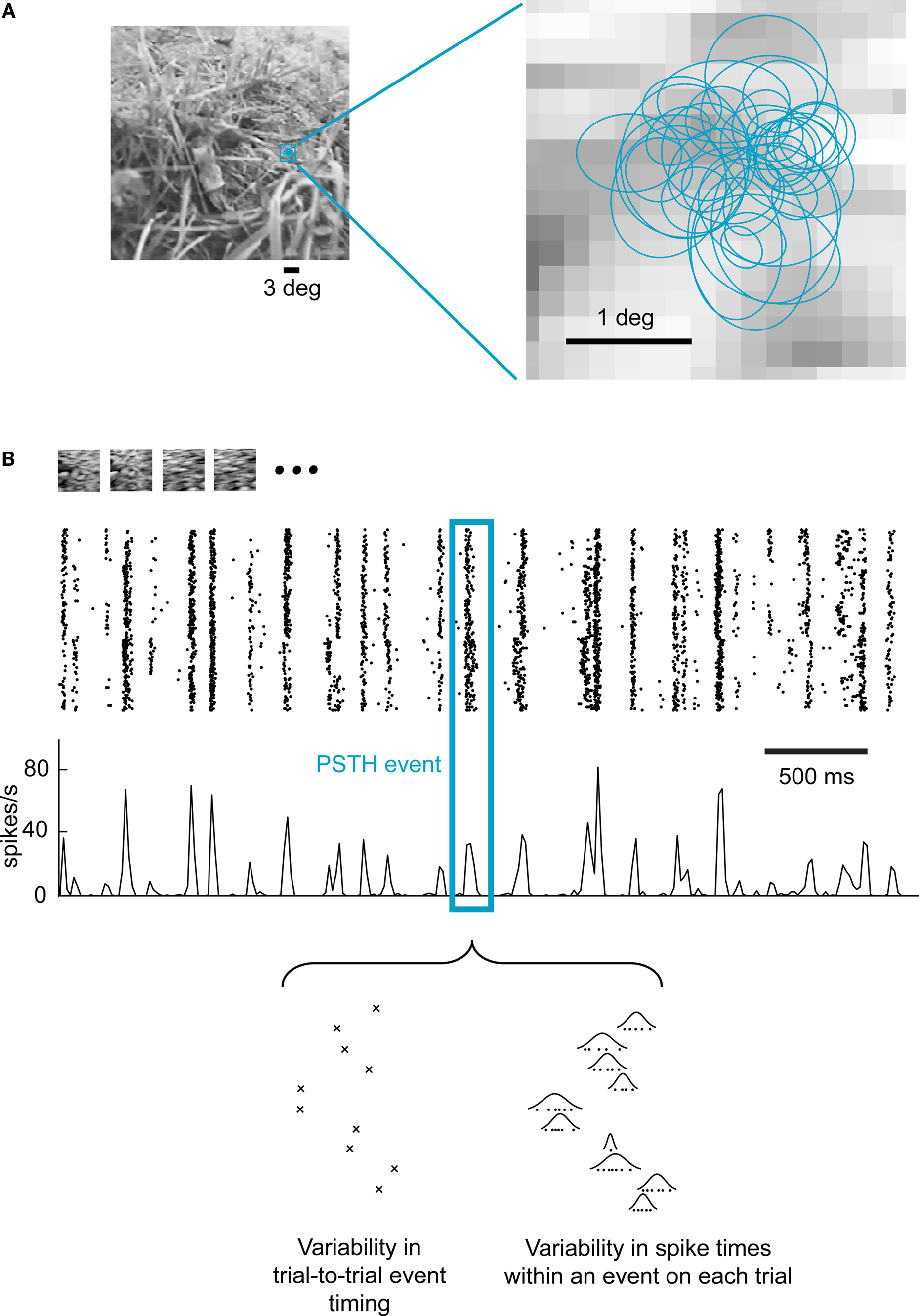
Figure 1. Event-like structure of LGN cell responses to natural scene movies. (A) A short section of a “cat-cam” movie was presented repeatedly to anesthetized cats while recording the extracellular activity of multiple single units in the LGN. The left panel shows the actual size of the receptive fields superimposed on one frame of the movie. The right panel shows in detail the receptive field location of all recorded cells (n = 37). Each receptive field is represented by the 1-standard deviation section of the 2D Gaussian that best fitted the spatial receptive field (see Materials and Methods). (B) Response of a single LGN neuron to 120 repeated presentations of a 4.2-s section of the movie. Each line in the raster plot corresponds to a single repeat (trial). Each dot represents the occurrence of an action potential. In the third row, the peri-stimulus time histogram (PSTH) shows the corresponding instantaneous firing rate, binned at intervals of one movie frame (17 ms). A single PSTH “event” (group of closely-spaced spikes) is highlighted to illustrate both sources of spike timing variability within each event (see Results), as previously described (Desbordes et al., 2008).

Previous modeling studies of early visual neurons have suggested that non stimulus-driven elements of neuronal firing are crucial in shaping the trial-averaged fine temporal precision of single cell response (Berry and Meister, 1998; Keat et al., 2001; Uzzell and Chichilnisky, 2004), which may be critical in faithfully encoding features of the more slowly varying natural scene (Butts et al., 2007). To systematically explore spiking precision in the context of event timing across trials and across neurons within a population, we turned to a generalized linear model (GLM) which incorporates not only stimulus-driven elements captured in the classical spatiotemporal receptive field but also non-stimulus elements captured in spike-history dependence (Paninski, 2004; Paninski et al., 2007; Pillow et al., 2008). In this framework, the firing activity is modeled as a conditionally Poisson process with a rate that depends on both the visual stimulus and the recent spiking activity. Note that this history dependence ensures that the response itself is strongly non-Poisson, with the global spike count variability lower than expected from Poisson statistics, as reported in neurons from the early visual system (Berry et al., 1997; Kara et al., 2000; Keat et al., 2001; Uzzell and Chichilnisky, 2004). The model fitting is then cast as a maximum likelihood estimation problem, a well-posed optimization problem for this framework (Paninski et al., 2007).

Figure 2 shows the model framework, which transforms the visual input (in the form of a spatiotemporal signal) into a series of spikes. The visual stimulus is first passed through a spatiotemporal filter corresponding to the classical receptive field of the neuron, which yields a temporal signal that we refer to as the filtered stimulus. This signal is then passed through a static exponential nonlinearity, resulting in the conditional intensity function which drives the Poisson spike generator. In the absence of spike-history dependence, the model reduces to the classical linear non-linear Poisson (LNP) model structure (Chichilnisky, 2001; Dayan and Abbott, 2001). In the full GLM, however, each generated spike is fed back through a spike history temporal filter and sums with the filtered stimulus, thereby modifying the conditional intensity function and potentially influencing the probability of future spiking. See Methods for more details on the model structure and fitting procedure.

FIGURE 2

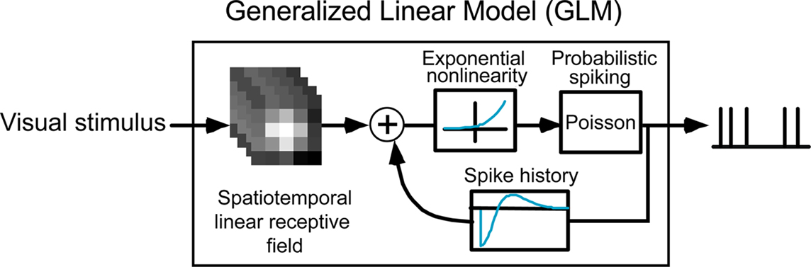
Figure 2. The generalized linear model (GLM). See “Materials and Methods” for details.

The model was fitted to LGN activity recorded extracellularly during presentation of a non-repeating spatiotemporal white noise movie. An example of a GLM fit to a typical LGN X ON cell is shown in Figure 3A, while the fits on all cells (n = 37) are summarized in Figure 3B. The spatiotemporal receptive fields were consistent with previous findings with a center-dominant, weak-surround spatial component and a biphasic temporal component. All spike history terms exhibited a short refractory period following the occurrence of a spike followed by an increase in probability of firing, as shown in Figure 3A (right panel and corresponding inset).

FIGURE 3

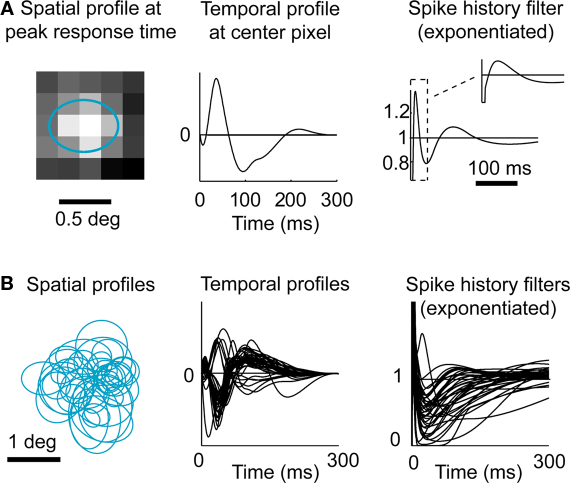
Figure 3. Fitting LGN responses with a Generalized Linear Model (GLM). (A) Model fit for a typical LGN X ON cell. In the model the linear receptive field is space–time inseparable, but here the spatial and temporal components are shown separately for simplicity. The spatial profile shown (left) corresponds to the spatial filter at the peak response time (with the 1-standard deviation contour of the best-fitting 2D Gaussian shown superimposed in blue), and the temporal profile shown (middle) is the temporal filter at the center of the RF. The exponential of the spike history temporal filter (right) is shown over the first 300 ms, and shown in more detail over the first 40 ms in inset. (B) Model fits for all cells (n = 37). Same conventions as in (A).

After fitting, the model was used to predict the neural response to the natural scene stimulus (not used for fitting), for comparison with the actual recorded responses of the cells. Figure 4A illustrates the response of a typical LGN X OFF cell to a short segment of the natural movie. The “event-like” patterns observed in the experimentally recorded cell response (first panel from the top) were captured by the GLM (second panel). They were also captured by the LNP model (third panel), here implemented as a GLM without the spike history component (h; see Materials and Methods) – consistent with the notion that the occurrence of events is tied to the visual stimulus (Butts et al., 2010).

FIGURE 4

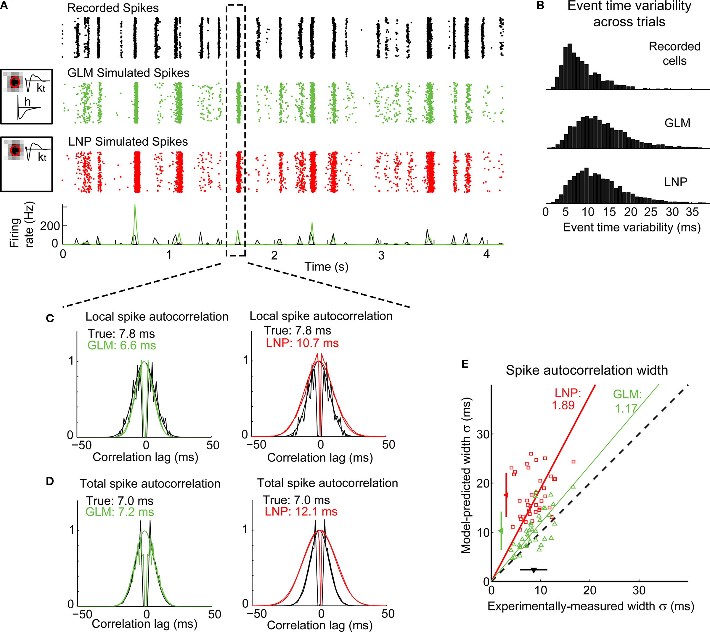
Figure 4. The GLM captures the fine timing precision of LGN cells in response to natural scenes. (A) Typical X OFF cell response to repeated presentations of a 4.2-s segment of the “cat-cam” movie. First row (black): Spikes recorded from this cell. Second row (green): Spikes predicted by the GLM fitted on this cell. The box on the left shows the model fits for this cell, with the spatial receptive field, the temporal profile (k_t) and the spike-history term (h). Third row (red): Spikes predicted by the LNP model fitted on this cell. The box on the left shows the fitted spatial receptive field and temporal profile (k_t). There is no spike history term in the LNP model. (B) Overall distribution of trial-to-trial event time variability across 120 repetitions of a 12.5-s movie for 29 LGN cells and 64 repetitions of a 10-s movie for 8 LGN cells (total: 598 events), in the experimentally recorded data (top) and in the simulated response of a GLM (middle) or LNP model (bottom) fitted to each cell. Event time variability is defined for each PSTH event as the standard deviation of the timing of the first spike, across all trials in which at least one spike occurred in this event. (C) Local spike autocorrelation functions for the cell shown in (A), computed locally from the spikes that constituted the event highlighted in the dashed box. Left: Prediction from the GLM (green) compared to the experimental measurement (black). Right: Prediction from the LNP model (red) compared to the experimental measurement (black). The numbers in inset indicate the temporal precision of the neural response as reflected in the spike autocorrelation width, defined as the standard deviation of the Gaussian function that best fits the autocorrelation function (which is also plotted). (D) Global spike autocorrelation functions for the cell shown in (A), computed on the full duration of the movie (12.5-s). Same conventions as in (C). (E) Spike autocorrelation widths for all cells (n = 37), as predicted by each model (red squares: LNP, green triangles: GLM) versus experimental measurements. The dashed line has unity slope. For each cell, the spike autocorrelation width is the standard deviation of the Gaussian that best fits the (global) spike autocorrelation function, as shown in (D) for an example case. For each model class, a fitted line and the corresponding proportionality coefficient are shown, computed between the experimentally measured autocorrelation width and the model-predicted width using a least-mean-square fit on all data points. The mean ± standard deviation are represented along each axis by an arrowhead and bar.

The cell responses during multiple repeats of this visual stimulus were summarized in the peri-stimulus time histogram (PSTH) which sums the responses across trials into a measure of instantaneous firing rate, here computed with a 17-ms bin (which is the duration of one frame of the visual stimulus). As illustrated at the bottom of Figure 4A, the PSTHs of the predicted cell response (green) and the experimentally recorded response (black) largely overlapped, indicating that the model was able to predict the occurrence of these events and their timing. For this cell, the correlation coefficient between the experimental and predicted PSTHs across 120 repeats was r = 0.39 for the GLM and r = 0.28 for the LNP model. Across all cells (n = 37), the correlation coefficient was 0.38 ± 0.18 (mean ± standard deviation) for the GLM and 0.36 ± 0.17 for the LNP model in the case of natural scenes stimuli, and 0.48 ± 0.19 for the GLM and 0.48 ± 0.19 for the LNP model in the case of spatiotemporal white noise. With this measure, both models gave similar performances that were consistent with the performances of previous models of LGN response designed at this relatively coarse time scale (Dan et al., 1996; Lesica and Stanley, 2004; Carandini et al., 2005; Lesica et al., 2007).

Given the episodic nature of the observed neural response, the recorded activity was parsed into discrete events (see Methods). We then computed for all events in all cells the difference between the average event time in the experimental data and that in the simulated data (where event time is defined as the time of the first spike in the event on a given trial). This time difference was less than 10 ms in 86% of the total number of non-empty events from all 37 cells (i.e., the events that contained at least one spike in at least one trial in both the experimental data and the simulated data, n = 5646), suggesting that the GLM could predict the average timing of an event with good accuracy. However, the LNP model performed just as well, with a time difference less than 10 ms in 86% of the total number of non-empty events (n = 5705). The variability of event time from trial to trial was also well captured by the models, as shown in Figure 4B. Defining event time variability as the standard deviation of the timing of the first spike in an event (across all trials in which the event contained at least one spike), we found that the distribution of event time variability was similar in the experimentally recorded cells (top panel) and in the GLM simulations (middle panel). In both cases it ranged between 0 and 25 ms, with a mean ± standard deviation of 8.3 ± 4.5 ms in the experimental data (n = 3086 non-empty events from 37 cells) and 13.3 ± 7.0 ms in the GLM prediction (n = 4026 non-empty events from 37 cells). The classic LNP model (bottom panel) gave a similar prediction of event time variability (12.8 ± 6.8 ms, n = 4087 non-empty events from 37 cells). These measurements suggest that both model structures could predict the timing of firing events and their variability across trials with a precision of approximately 10–20 ms.

Taken together, the existence of event-like response structure, the timing of the response events, and the variations in event times across trials were reasonably well predicted by the stimulus-driven element of the modeling framework (i.e., the model part shared by the LNP model and the GLM). The importance of the non-stimulus driven component of the response emerged, however, in the analysis of the spike autocorrelation function (Figures 4C,D). The autocorrelation function quantifies the temporal relationship between neighboring spikes on a trial-by-trial basis by indicating, given a spike at time 0, the probability of other spikes occurring shortly before (negative lags) or after (positive lags) (see Methods). On the left panel of Figure 4C are the actual (black) and GLM-predicted (green) spike autocorrelation functions for the event highlighted in Figure 4A, illustrating that the GLM captured the fine temporal precision of this event (6.6 ms predicted width versus 7.8 ms experimentally measured width). The lack of short inter-spike intervals, indicative of neural refractoriness, was also well captured through the spike-history dependence embedded in the model, as explained below. Note that in addition to the spike autocorrelation function for the GLM prediction, superimposed is the best Gaussian fit to the autocorrelation function. In contrast, the LNP model (right panel of Figure 4C) significantly under-estimated the local timing precision (or over-estimated the spread of spiking on a particular trial, 10.7 ms predicted width versus 7.8 ms experimentally measured width) due to the absence of the spike-history dependent element. These results were consistent when the measures for this cell were repeated across all events within the sequence, as shown in Figure 4D.

When applied across a larger sample of neurons (n = 37), the GLM captured the precision of spike timing, as shown in the scatter plot of observed versus predicted autocorrelation widths in Figure 4E (green triangles). When the spike-history dependence was removed, however, the LNP model prediction (red squares) significantly differed from the experimental observation. Note that both models captured the mean firing rates of the actual neurons (paired t-test, p > 0.1 for all pairwise comparisons of the mean firing rate of experiment versus model). We also tested the model on a different stimulus class, spatiotemporal white noise, and found similar results (see Figures 5A,B).

FIGURE 5

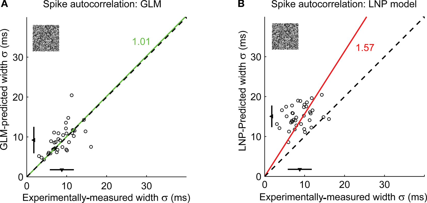
Figure 5. The GLM captures the fine timing precision of LGN cells in response to spatiotemporal white noise stimuli. (A) Spike autocorrelation widths for all cells (n = 37), as predicted by the GLM versus experimental measurements. The dashed line has unity slope. For each cell, the spike autocorrelation width is the standard deviation of the Gaussian that best fits the (global) spike autocorrelation function. A fitted line (green) and the corresponding proportionality coefficient are shown, computed between the experimentally measured autocorrelation width and the model-predicted width using a least-mean-square fit on all data points. The mean ± standard deviation are represented along each axis by an arrowhead and bar. The model predictions are not significantly different from the experimental measurements (paired t-test: p = 0.36). (B) Same as (A), but as predicted by the LNP model. The LNP model significantly overestimates the autocorrelation width (paired t-test: p < 10⁻¹²).

The GLM, therefore, with a specific mechanism for capturing spike-history dependence, was more predictive of the fine timing precision in LGN cells when not obscured by averaging across trials. This mechanism is illustrated in Figure 6, where the conditional intensity functions for both the GLM and LNP model are shown for several trials. For the LNP, the conditional intensity function is solely a function of the visual stimulus, and therefore is identical from trial to trial (Figure 6A). The variability in the timing of events is simply due to the intrinsic variability of the Poisson spike generator. In contrast, the GLM conditional intensity function is modified in each trial by the presence and timing of each generated spike (Figure 6B). Every time a spike occurs, the conditional intensity function is updated to a much lower value, reflecting the fact that an immediately subsequent spike is very unlikely (due to short term refractoriness). After a few milliseconds, however, the probability rises to a new level which is higher than before the spike, making it more likely that another spike will soon follow. This is all consistent with the shape of the spike history function showing a less-than-unity gain shortly after 0 followed by a greater-than-one rebound (Figure 6C). This rebound facilitates the generation of spikes that follow each other quickly, and hence is consistent with a narrower spike autocorrelation function (Figures 4C–E).

FIGURE 6

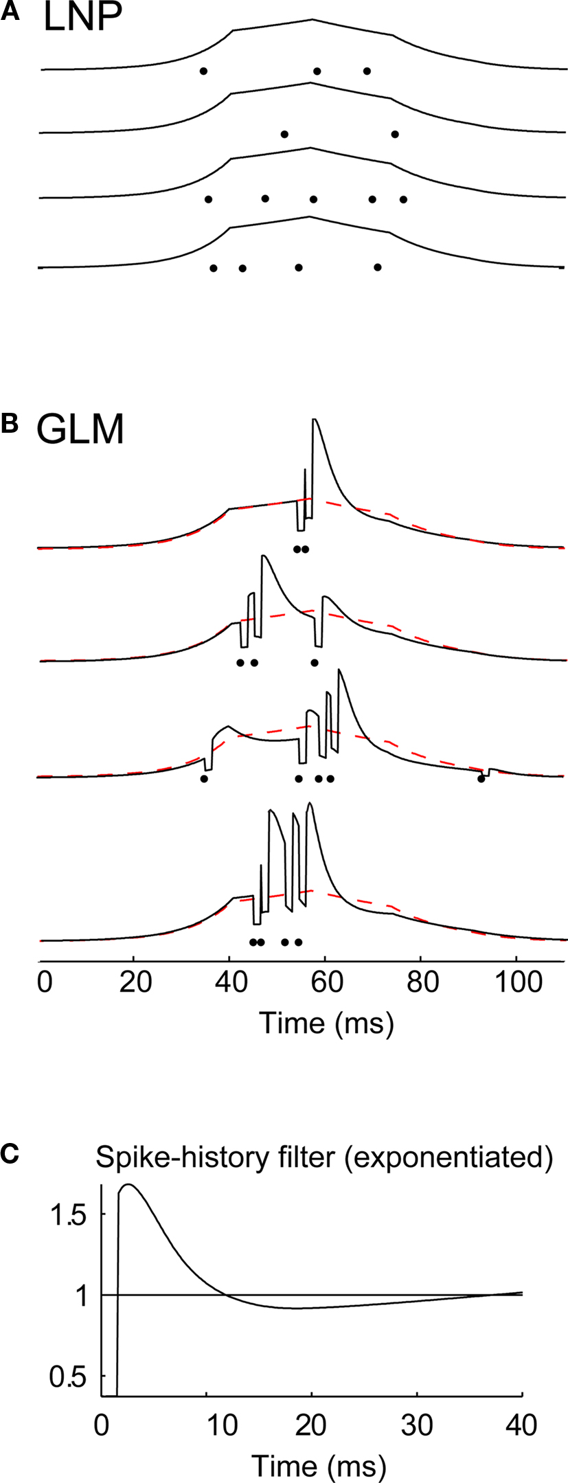
Figure 6. The influence of spike history on spike timing within firing events. (A) Conditional intensity functions associated with a local event for four different trials generated by the LNP model fitted to an X-ON cell, for a given 100-ms period in the movie stimulus. For each trial the conditional intensity function (black curve) is plotted along with the resulting spikes (black dots). (B) Conditional intensity functions generated by the GLM fitted on the same cell, along with the corresponding spikes generated by the model, for four repetitions of the same 100-ms period in the movie. The conditional intensity function from the LNP model in (A) is superimposed for comparison (dashed red curve). Same conventions as in (A). (C) Spike-history filter for this cell (after exponentiation), as fitted with the GLM. The filter is shown for the first 40 ms to highlight the effects of spike history on a short-time scale.

Perhaps even more interestingly – since the model was fit on a different stimulus class (spatiotemporal white noise) at high contrast – the model was able to predict the cell responses for natural scenes at low (15%) contrast as well as or even better than at high (40%) contrast. Across all cells (n = 37), the correlation coefficient at low contrast was 0.44 ± 0.21 (mean ± standard deviation), compared to 0.38 ± 0.18 at high contrast. The model was able to predict the contrast-invariant nature of spike timing precision within events (Figure 7, green triangles), which we previously reported (Desbordes et al., 2008). This was not the case for the LNP model, which not only failed dramatically at capturing fine spike timing precision, but incorrectly predicted a degraded precision at low contrast (Figure 7, red squares). The failure of the LNP model was expected since it could only match the PSTH of the cell response, and not the finer details of spike timing within events. As we previously showed, PSTH events have a longer duration at low contrast than high contrast because the timing of events is more variable (across repeats) at low contrast, even though the timing of spikes within events is not (Desbordes et al., 2008). Therefore, it is not surprising that the LNP model would incorrectly predict a degraded precision at low contrast. This result suggests that the differences in the geniculate response at different contrast levels can be well captured through the nonlinear interactions between the natural scene and the spike-history dependence, even when fitting the model at a single contrast level.

FIGURE 7

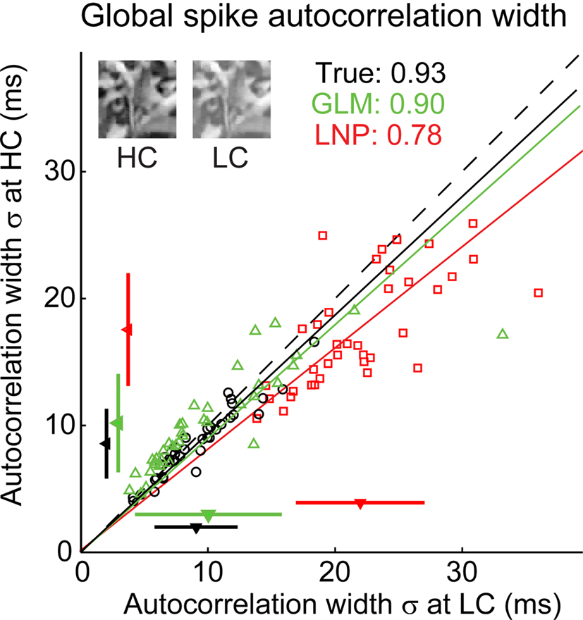
Figure 7. The GLM predicts the contrast-invariance of timing precision in LGN cells. Temporal precision measured as the global spike autocorrelation width in response to natural scenes at high contrast (HC; 40% RMS contrast) versus low contrast (LC; 15% RMS contrast), for the GLM prediction (green triangles), the LNP model prediction (red squares), and the experimental measurements (black circles). The dashed line has unity slope. For each of the three sets of points, a fitted line of the same color and the corresponding proportionality coefficient are shown, computed between the autocorrelation width measured at HC and that measured at LC using a least-mean-square fit on all data points. The mean ± standard deviation are represented along each axis by an arrowhead and bar.

We now turn to the question of the relative timing of firing activity across neurons within the population. Figure 8A shows the simultaneously recorded responses of two neighboring neurons to the natural movie (denoted as “Exp.” in the raster), below which are the corresponding rasters of the GLM simulation for each neuron. Timing precision in the population code can be estimated by the width of the cross-correlation between the activity of pairs of cells (Desbordes et al., 2008), which gives the probability of neuron 2 spiking at various time lags relative to a spike in neuron 1. Note that this quantity is typically measured as an average across the full duration of a visual stimulus, with the assumption of stationarity. In natural scenes, however, stimulus-driven correlation (and thus spike timing precision) across cells is not constant, but rather varies continually as the visual stimulus changes.

FIGURE 8

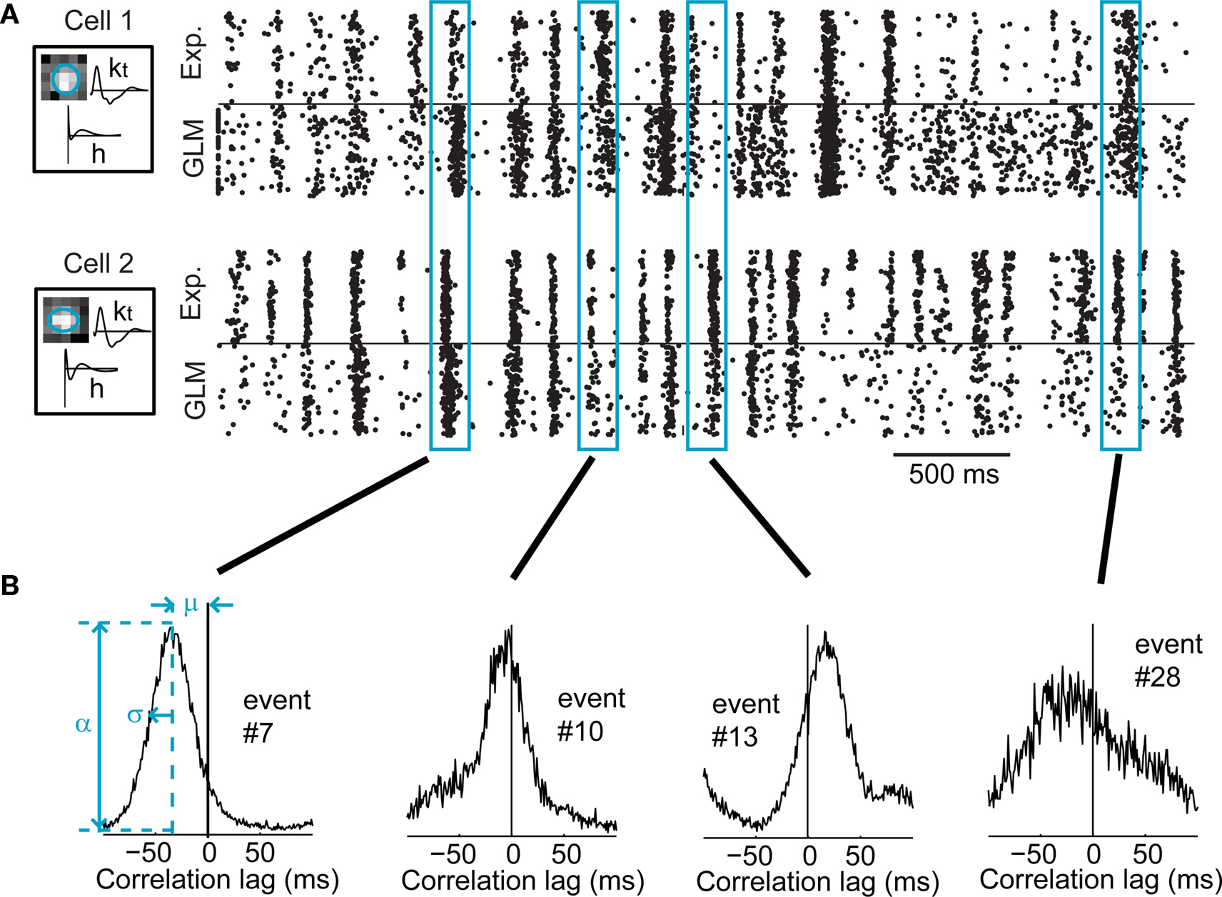
Figure 8. Activity of a typical pair of LGN cells exhibiting stimulus-induced cross-correlation in their response. (A) Raster plots of the responses of two LGN cells, and their respective GLM simulations, for 120 repeated presentations of a 4.2-s segment of the natural scenes movie. The boxes on the left show the model fits for these cells, with the spatial receptive field, the temporal profile (k_t), and the spike-history term (h). (B) Typical local cross-correlation functions computed from GLM simulations of four different events shared by the two above cells. Whereas only 120 simulated trials are shown in (A), 10,000 trials were simulated to compute these local cross-correlations. The left panel shows how the peak correlation value (α), the mean latency (μ), and the cross-correlation width (σ, the standard deviation of the best-fitting Gaussian) were defined.

In Figure 8A, both cells had neighboring receptive fields and tended to respond at similar times to the stimulus features, making it possible to identify events that were aligned across both cells (see Methods). Four particular events are highlighted here. The local spike cross-correlation was computed for each of these four events (Figure 8B), based on model-generated spikes as explained below. It can be qualitatively seen that the local cross-correlations varied in several ways, perhaps most importantly in terms of the mean local latency (μ) between the firing of the two neurons (e.g., in event #7, cell 1 tended to consistently fire before cell 2), and of the width (σ) of the cross-correlation function which captures the temporal precision of synchronous firing across the cells. The correlation function width (σ), peak value (α), and mean latency (μ) took different values in these four events, highlighting the degree of modulation in the relative firing across cells in the population.

The reliable estimation of temporally localized correlation structure requires a very large number of spikes, often unattainable experimentally. For a small number of events, however, the localized cross-correlation could be measured in the experimental data, and was reliably predicted by the GLM (Figure 9). Given the ability of the GLM to predict local cross-correlations for these examples and to predict the activity of each neuron individually, we used the GLM to generate spike trains from each cell in response to 10,000 repetitions of the visual stimulus (see Methods), a number largely sufficient to yield smooth estimates of the local cross-correlation between cells on an event-by-event basis, over all events shared by a pair of cells.

FIGURE 9

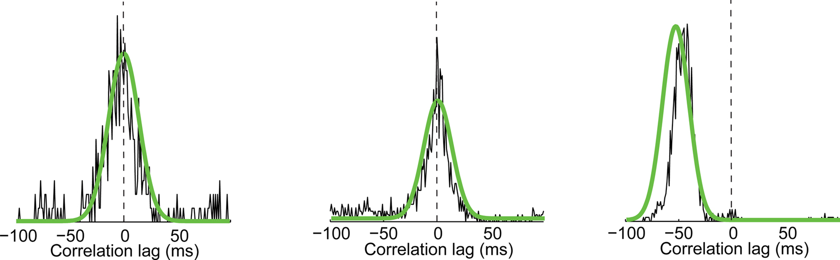
Figure 9. Three examples of events shared across two cells for which 120 repeats are sufficient to measure the width of the local cross-correlation. Experimental measurements for three different events recorded in three different pairs of cells. Superimposed in green are the predictions of the GLM model for 10,000 repeats simulating the same three pairs at those particular events.

A summary of the variability in the shape of local cross-correlation functions is shown in Figure 10A for the same pair of cells as in Figure 8. The local cross-correlation functions for all events (black curves) are superimposed with the global cross-correlation computed on the full stimulus duration (dashed blue curve). Across all 38 pairs, there was a wide distribution of event-by-event cross-correlation widths (σ; Figure 10B) and of mean latencies (μ; Figure 10C). See figure caption for statistics. As a validation, the global temporal precision across cell pairs averaged across the entire natural scene movie was estimated using the GLM, resulting in predictions that were consistent with our previously reported experimental measurements (Desbordes et al., 2008), as shown in Figure 11A. Even though the cross-correlation widths in the model prediction and in the experimental data slightly differed (paired t-test, p = 0.006, n = 37 cells), the best-fitting ratio between model prediction and experimental measurement was 1.10 (Figure 11A), corresponding to an error of only 10%, suggesting that the GLM was indeed a good predictor of correlations across geniculate neurons in response to natural scene stimuli. Not surprisingly, the GLM performed even better in the case of spatiotemporal white noise (Figure 11B), where the model predictions were not significantly different from the experimental measurements (paired t-test: p = 0.36), with a ratio of 0.96.

FIGURE 10

Figure 10. Local variations in the temporal precision across LGN neurons. (A) Local (black) and global (dashed blue) cross-correlation functions for the pair of cells shown in Figure 8. (B) Distribution of values of local cross-correlation width (σ) in all 38 cell pairs, for all shared events in which the peak of the cross-correlation function (α) was higher than 0.005 (n = 321 events, median = 14.3 ms, mean = 15.4 ms, standard deviation = 4.8 ms). (C) Distribution of values of mean latency (μ) in all 38 cell pairs, for all shared events in which the peak of the local cross-correlation function (α) was higher than 0.005 (n = 321 events, median = −1.2 ms, mean = −1.9 ms, standard deviation = 22.7 ms).

FIGURE 11

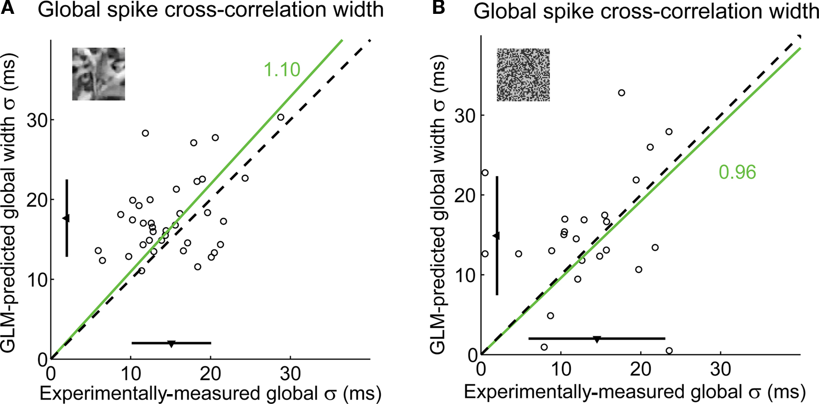
Figure 11. The GLM globally captures the fine timing precision across cells. (A) Global spike cross-correlation width in response to natural scenes, as predicted by the GLM versus as measured in experimental data (correlation coefficient: r = 0.41). For each pair, the spike cross-correlation width is the standard deviation of the Gaussian that best fits the (global) spike cross-correlation function. A fitted line (green) and the corresponding proportionality coefficient are shown, computed between the cross-correlation width predicted by the GLM and that measured experimentally using a least-mean-square fit on all data points. The mean ± standard deviation are represented along each axis by an arrowhead and bar. The dashed line has unity slope. (B) Global spike cross-correlation width in response to spatiotemporal white noise, as predicted by the GLM versus measured in experimental data, in all pairs in which there was a measurable hump in the cross-correlation for this class of visual stimuli (n = 24 pairs). Same conventions as in (A).

4 Discussion

In response to natural scenes, early visual neurons tend to fire in a characteristic manner, with firing “events” (i.e., small clusters of spikes) clearly separated by periods of silence (Dan et al., 1996; Berry et al., 1997; Reinagel and Reid, 2000; Keat et al., 2001). We recently showed that in the case of natural visual stimuli the responses of neurons in the LGN exhibit a temporal precision of 10–25 ms within and across cells in the geniculate population (Desbordes et al., 2008), a time scale significantly faster than would be predicted by the more slowly varying natural scene (Butts et al., 2007). Here, we used a spiking model of neural encoding based on a generalized linear model framework with spike history dependence to fit the responses of LGN neurons. With this model, we investigated variations in temporal precision of thalamic population responses to natural scene stimuli. We showed that the model could predict the experimental measurements of geniculate responses to natural stimuli, not only capturing the global correlation structure measured across the entire stimulus duration, but also the local correlation structure at the scale of individual firing events. The model was able to capture the occurrence of firing events, the timing of these events and their variability, and the finer details of spikes within an event. Measurements across the population revealed the continuous modulation of the relative timing of activity across neurons in a 5–25 ms range.

Functional models have been used previously to predict early visual neuron response to natural scene stimuli (Carandini et al., 2005; Lesica et al., 2007; Mante et al., 2008). In the case of the standard LNP model, the cell response is solely due to modulations by the visual stimulus, thus the time scale of the neural activity is limited to the time scale of the input. The LNP model does capture the coarse nature of the observed response to natural scene inputs (Lesica et al., 2007), but requires fitting on natural scene data and does not generalize well across different stimulus conditions. We previously showed that within the LNP modeling framework, the spatiotemporal filtering and the threshold properties of the nonlinearity differ across stimulus classes such that LNP models fit to spatiotemporal white noise data do not predict well the geniculate response to natural scenes (Lesica et al., 2007). Here, by fitting the GLM on the neural response to spatiotemporal white noise stimuli and testing it on natural scene stimuli, we show that the expansion of the framework to include the non stimulus-driven spike-history dependence embodies an important element missing from the conventional LNP framework in the context of natural scene stimuli. This suggests that interactions between the natural scene inputs and the nonlinearity of the spike-history dependence make it possible to capture the important differences in cell response that would manifest as threshold shifts in the simpler LNP model framework. Importantly, fitting the GLM to high-contrast spatiotemporal white noise data generalized to natural scenes at different contrasts, exhibiting the contrast-invariance in the relative timing of geniculate neurons that we have previously shown experimentally (Desbordes et al., 2008). The LNP model, however, showed more dependence on contrast and was thus unable to capture the observed phenomena with a single set of model parameters. Taken together, these results suggest that the augmentation of the classical (LNP) modeling framework with non stimulus-driven spike-history dependence expands the generality of the model to allow complex interactions between properties of the stimulus and the nonlinear dependence of spiking upon both visual stimulation and past activity.

The importance of spike history (or recovery) in shaping a cell’s fine temporal precision was previously emphasized in models of retinal firing (Berry and Meister, 1998; Keat et al., 2001; Uzzell and Chichilnisky, 2004; Pillow et al., 2005). In contrast to the GLM presented here, in these models, the visual stimulus consisted of a one-dimensional time series and was passed through a linear (or linear–nonlinear) temporal filter, whose output (after driving an integrate-and-fire mechanism in the case of Keat et al., 2001) was fed back through a recovery function to influence the subsequent integration and thus future firing. These models were fitted to the activity of individual retinal ganglion cells and LGN neurons in response to temporally-white noise stimulus (often referred to as “full-field flicker”), and predicted the narrow PSTH events observed experimentally. Here, in a more general spatiotemporal modeling framework, we showed the interactions between spike history and the complex spatial and temporal structure of natural scenes across a population of LGN cells.

In the retina, previous studies suggest the existence of a significant degree of correlated (or synchronous) firing, often referred to as “noise correlations” because they cannot be explained solely by the visual input to each cell independently (Mastronarde, 1983a,b; Meister et al., 1995; DeVries, 1999). Synchronized firing in the retina varies with cell types and appears to be mediated by a combination of mechanisms: direct gap junction coupling between neighboring retinal ganglion cells, gap junction coupling through interneurons (e.g., amacrine cells), and chemical synapses providing common input to retinal ganglion cells from bipolar or amacrine cells (reviewed in Baccus, 2007; Demb, 2007; Field and Chichilnisky, 2007). Common synaptic input seems to be the dominant source of synchronous firing in the retina – probably due to a single noise source, namely photoreceptor noise (Trong and Rieke, 2008). However, while the existence of these noise correlations in the retina is well documented, their importance for neural encoding and decoding of the visual input has been controversial (Meister et al., 1995; Meister, 1996; Nirenberg et al., 2001; Nirenberg and Latham, 2003; Schneidman et al., 2003; Latham and Nirenberg, 2005; Puchalla et al., 2005). In a recent study, a generalized linear model accounting for pairwise coupling among neighboring retinal ganglion cells could better fit cross-correlation functions and could extract ≈20% more information about the visual stimulus than the uncoupled version of the model (Pillow et al., 2008), favoring the hypothesis that noise correlations in the retina contribute at least some information about the visual stimulus.

In the next visual processing stage – the LGN – which is the focus of this study, neighboring neurons typically do not exhibit high noise correlations (unless they share a retinal afferent, as detailed below), and the relevance of these correlations for the representation of natural visual scenes is unclear. Our present and previous results suggest that noise correlations are weaker overall in the LGN than in the retina, especially in the presence of natural scene stimulation (Desbordes et al., 2008), with the exception of cell pairs sharing a retinal afferent which are instead very strongly correlated on a short (1-ms) time scale (Alonso et al., 1996, 2008; Yeh et al., 2009). The lower amount of noise correlation in the LGN may be due to the fact that the local neural circuitry in the LGN is very different from that in the retina. There is no evidence of direct excitatory connections between LGN cells and it is likely that noise correlations only exist between cells that receive some amount of common retinal input from the same afferent (Alonso et al., 1996; Usrey et al., 1998). In summary, direct coupling between neighboring cells, modeled in the retina with pairwise reciprocal spike history terms (Pillow et al., 2008), was not relevant in the LGN population activity described here.

Fine temporal precision in early visual neurons is necessary for the faithful representation of the more slowly varying natural visual scene (Butts et al., 2007). The results presented here point to the importance of spiking history in shaping temporal precision of the neural code and thus in maintaining a high fidelity of scene representation. Modulation of the relative timing of spikes across the population was found both in the mean latency between one cell and another and in the variability of firing around this mean. Previous studies have shown the sensitivity of the thalamocortical synapse for synchronous activity in the thalamic input (Alonso et al., 1996; Dan et al., 1998; Usrey and Reid, 1999; Kara and Reid, 2003; Bruno and Sakmann, 2006; Kumbhani et al., 2007), hinting at the importance of precise timing for cortical selectivity to particular patterns of luminance changes associated with motion in natural visual scenes.

Since fine precision in spike timing may be crucial to neural coding in other brain areas (Rieke et al., 1996; Lestienne, 2001), we hypothesize that the relative timing of spikes is similarly modulated by natural stimuli in other brain areas, along the visual pathway and in other modalities. Given the limited predictive power of the LNP model, the GLM framework may offer an improved approach to this question for future studies.

Conflict of Interest Statement

The authors declare that the research was conducted in the absence of any commercial or financial relationships that could be construed as a potential conflict of interest.

Acknowledgments

We would like to thank Jonathan Pillow for sharing code and for helpful comments on model fitting, Dan Butts for help with the event analysis, and members of the Stanley group for useful comments on the manuscript. This work was supported by NSF CRCNS Grant IIS-0904630 (GBS, JMA), and the National Eye Institute EY005253 (JMA).

References

Alonso, J. M., Usrey, W. M., and Reid, R. C. (1996). Precisely correlated firing in cells of the lateral geniculate nucleus. Nature 383, 815–819.

Pubmed Abstract | Pubmed Full Text | CrossRef Full Text

Alonso, J. M., Yeh, C. I., and Stoelzel, C. R. (2008). Visual stimuli modulate precise synchronous firing within the thalamus. Thalamus Relat. Syst. 4, 21–34.

Pubmed Abstract | Pubmed Full Text | CrossRef Full Text

Atick, J. J., and Redlich, A. (1992). What does the retina know about natural scenes? Neural. Comput. 4, 196–210.

CrossRef Full Text

Avissar, M., Furman, A. C., Saunders, J. C., and Parsons, T. D. (2007). Adaptation reduces spike-count reliability, but not spike-timing precision, of auditory nerve responses. J. Neurosci. 27, 6461–6472.

Pubmed Abstract | Pubmed Full Text | CrossRef Full Text

Baccus, S. A. (2007). Timing and computation in inner retinal circuitry. Annu. Rev. Physiol. 69, 271–290.

Pubmed Abstract | Pubmed Full Text | CrossRef Full Text

Barbieri, R., Quirk, M. C., Frank, L. M., Wilson, M. A., and Brown, E. N. (2001). Construction and analysis of non-Poisson stimulus-response models of neural spiking activity. J. Neurosci. Methods 105, 25–37.

Pubmed Abstract | Pubmed Full Text | CrossRef Full Text

Berry, M. J., and Meister, M. (1998). Refractoriness and neural precision. J. Neurosci. 18, 2200–2211.

Pubmed Abstract | Pubmed Full Text

Berry, M. J., Warland, D. K., and Meister, M. (1997). The structure and precision of retinal spike trains. Proc. Natl. Acad. Sci. U.S.A. 94, 5411–5416.

Pubmed Abstract | Pubmed Full Text | CrossRef Full Text

Brillinger, D. R., Bryant, H.L. Jr., and Segundo, J. P. (1976). Identification of synaptic interactions. Biol. Cybern. 22, 213–228.

Pubmed Abstract | Pubmed Full Text | CrossRef Full Text

Brody, C. D. (1999). Correlations without synchrony. Neural. Comput. 11, 1537–1551.

Pubmed Abstract | Pubmed Full Text | CrossRef Full Text

Bruno, R. M., and Sakmann, B. (2006). Cortex is driven by weak but synchronously active thalamocortical synapses. Science 312, 1622–1627.

Pubmed Abstract | Pubmed Full Text | CrossRef Full Text

Butts, D. A., Desbordes, G., Weng, C., Jin, J., Alonso, J.-M., and Stanley, G. B. (2010). The episodic nature of spike trains in the early visual pathway. J. Neurophysiol. doi:10.1152/jn.00078.2010

Pubmed Abstract | Pubmed Full Text | CrossRef Full Text

Butts, D. A., Weng, C., Jin, J., Yeh, C. I., Lesica, N. A., Alonso, J. M., and Stanley, G. B. (2007). Temporal precision in the neural code and the timescales of natural vision. Nature 449, 92–95.

Pubmed Abstract | Pubmed Full Text | CrossRef Full Text

Carandini, M., Demb, J. B., Mante, V., Tolhurst, D. J., Dan, Y., Olshausen, B. A., Gallant, J. L., and Rust, N. C. (2005). Do we know what the early visual system does? J. Neurosci. 25, 10577–10597.

Pubmed Abstract | Pubmed Full Text | CrossRef Full Text

Chichilnisky, E. J. (2001). A simple white noise analysis of neuronal light responses. Network 12, 199–213.

Pubmed Abstract | Pubmed Full Text

Dan, Y., Alonso, J. M., Usrey, W. M., and Reid, R. C. (1998). Coding of visual information by precisely correlated spikes in the lateral geniculate nucleus. Nat. Neurosci. 1, 501–507.

Pubmed Abstract | Pubmed Full Text | CrossRef Full Text

Dan, Y., Atick, J. J., and Reid, R. C. (1996). Efficient coding of natural scenes in the lateral geniculate nucleus: experimental test of a computational theory. J. Neurosci. 16, 3351–3362.

Pubmed Abstract | Pubmed Full Text

Dayan, P., and Abbott, L. F. (2001). Theoretical Neuroscience: Computational and Mathematical Modeling of Neural Systems. MIT Press, Cambridge, MA.

Demb, J. B. (2007). Cellular mechanisms for direction selectivity in the retina. Neuron 55, 179–186.

Pubmed Abstract | Pubmed Full Text | CrossRef Full Text

Dempster, A., Laird, N., and Rubin, D. (1977). Maximum likelihood from incomplete data via the EM algorithm. J. R. Stat. Soc. 39, 1–38.

Desbordes, G., Jin, J., Weng, C., Lesica, N. A., Stanley, G. B., and Alonso, J. M. (2008). Timing precision in population coding of natural scenes in the early visual system. PLoS Biol. 6, e324. doi: 10.1371/journal.pbio.0060324.

Pubmed Abstract | Pubmed Full Text | CrossRef Full Text

DeVries, S. H. (1999). Correlated firing in rabbit retinal ganglion cells. J. Neurophysiol. 81, 908–920.

Pubmed Abstract | Pubmed Full Text

Dong, D. W., and Atick, J. J. (1995). Statistics of natural time-varying images. Netw. Comput. Neural Syst. 6, 345–358.

CrossRef Full Text

Field, D. J. (1987). Relations between the statistics of natural images and the response properties of cortical cells. J. Opt. Soc. Am. Optic. Image Sci. 4, 2379–2394.

CrossRef Full Text

Field, G. D., and Chichilnisky, E. J. (2007). Information processing in the primate retina: circuitry and coding. Annu. Rev. Neurosci. 30, 1–30.

Pubmed Abstract | Pubmed Full Text | CrossRef Full Text

Kara, P., and Reid, R. C. (2003). Efficacy of retinal spikes in driving cortical responses. J. Neurosci. 23, 8547–8557.

Pubmed Abstract | Pubmed Full Text

Kara, P., Reinagel, P., and Reid, R. C. (2000). Low response variability in simultaneously recorded retinal, thalamic, and cortical neurons. Neuron 27, 635–646.

Pubmed Abstract | Pubmed Full Text | CrossRef Full Text

Kayser, C., Einhauser, W., and Konig, P. (2003). Temporal correlations of orientations in natural scenes. Neurocomputing 52, 117–123.

CrossRef Full Text

Keat, J., Reinagel, P., Reid, R. C., and Meister, M. (2001). Predicting every spike: a model for the responses of visual neurons. Neuron 30, 803–817.

Pubmed Abstract | Pubmed Full Text | CrossRef Full Text

Kumbhani, R. D., Nolt, M. J., and Palmer, L. A. (2007). Precision, reliability, and information-theoretic analysis of visual thalamocortical neurons. J. Neurophysiol. 98, 2647–2663.

Pubmed Abstract | Pubmed Full Text | CrossRef Full Text

Latham, P. E., and Nirenberg, S. (2005). Synergy, redundancy, and independence in population codes, revisited. J. Neurosci. 25, 5195–5206.

Pubmed Abstract | Pubmed Full Text | CrossRef Full Text

Lesica, N. A., Jin, J., Weng, C., Yeh, C. I., Butts, D. A., Stanley, G. B., and Alonso, J. M. (2007). Adaptation to stimulus contrast and correlations during natural visual stimulation. Neuron 55, 479–491.

Pubmed Abstract | Pubmed Full Text | CrossRef Full Text

Lesica, N. A., and Stanley, G. B. (2004). Encoding of natural scene movies by tonic and burst spikes in the lateral geniculate nucleus. J. Neurosci. 24, 10731–10740.

Pubmed Abstract | Pubmed Full Text | CrossRef Full Text

Lestienne, R. (2001). Spike timing, synchronization and information processing on the sensory side of the central nervous system. Prog. Neurobiol. 65, 545–591.

Pubmed Abstract | Pubmed Full Text | CrossRef Full Text

Mainen, Z. F., and Sejnowski, T. J. (1995). Reliability of spike timing in neocortical neurons. Science 268, 1503–1506.

Pubmed Abstract | Pubmed Full Text | CrossRef Full Text

Mante, V., Bonin, V., and Carandini, M. (2008). Functional mechanisms shaping lateral geniculate responses to artificial and natural stimuli. Neuron 58, 625–638.

Pubmed Abstract | Pubmed Full Text | CrossRef Full Text

Mastronarde, D. N. (1983a). Correlated firing of cat retinal ganglion cells. II. Responses of X- and Y-cells to single quantal events. J. Neurophysiol. 49, 325–349.

Mastronarde, D. N. (1983b). Correlated firing of cat retinal ganglion cells. I. Spontaneously active inputs to X- and Y-cells. J. Neurophysiol. 49, 303–324.

Meister, M. (1996). Multineuronal codes in retinal signaling. Proc. Natl Acad. Sci. U.S.A. 93, 609–614.

Pubmed Abstract | Pubmed Full Text | CrossRef Full Text

Meister, M., Lagnado, L., and Baylor, D. A. (1995). Concerted signaling by retinal ganglion cells. Science 270, 1207–1210.

Pubmed Abstract | Pubmed Full Text | CrossRef Full Text

Nirenberg, S., Carcieri, S. M., Jacobs, A. L., and Latham, P. E. (2001). Retinal ganglion cells act largely as independent encoders. Nature 411, 698–701.

Pubmed Abstract | Pubmed Full Text | CrossRef Full Text

Nirenberg, S., and Latham, P. E. (2003). Decoding neuronal spike trains: how important are correlations? Proc. Natl. Acad. Sci. U.S.A. 100, 7348–7353.

Pubmed Abstract | Pubmed Full Text | CrossRef Full Text

Paninski, L. (2004). Maximum likelihood estimation of cascade point-process neural encoding models. Network 15, 243–262.

Pubmed Abstract | Pubmed Full Text | CrossRef Full Text

Paninski, L., Pillow, J., and Lewi, J. (2007). Statistical models for neural encoding, decoding, and optimal stimulus design. Prog. Brain Res. 165, 493–507.

Pubmed Abstract | Pubmed Full Text | CrossRef Full Text

Park, I., Paiva, A. R., Demarse, T. B., and Principe, J. C. (2008). An efficient algorithm for continuous time cross correlogram of spike trains. J. Neurosci. Methods 168, 514–523.

Pubmed Abstract | Pubmed Full Text | CrossRef Full Text

Perkel, D. H., Gerstein, G. L., and Moore, G. P. (1967). Neuronal spike trains and stochastic point processes. I. The single spike train. Biophys. J. 7, 391–418.

Pubmed Abstract | Pubmed Full Text | CrossRef Full Text

Pillow, J. W., Paninski, L., Uzzell, V. J., Simoncelli, E. P., and Chichilnisky, E. J. (2005). Prediction and decoding of retinal ganglion cell responses with a probabilistic spiking model. J. Neurosci. 25, 11003–11013.

Pubmed Abstract | Pubmed Full Text | CrossRef Full Text

Pillow, J. W., Shlens, J., Paninski, L., Sher, A., Litke, A. M., Chichilnisky, E. J., and Simoncelli, E. P. (2008). Spatio-temporal correlations and visual signalling in a complete neuronal population. Nature 454, 995–999.

Pubmed Abstract | Pubmed Full Text | CrossRef Full Text

Puchalla, J. L., Schneidman, E., Harris, R. A., and Berry, M. J. (2005). Redundancy in the population code of the retina. Neuron 46, 493–504.

Pubmed Abstract | Pubmed Full Text | CrossRef Full Text

Reinagel, P., and Reid, R. C. (2000). Temporal coding of visual information in the thalamus. J. Neurosci. 20, 5392–5400.

Pubmed Abstract | Pubmed Full Text

Rieke, F., Warland, D., de Ruyter van Steveninck, R., and Bialek, W. (1996). Spikes: Exploring the Neural Code. Cambridge: The MIT Press.

Schneidman, E., Bialek, W., and Berry, M. J. (2003). Synergy, redundancy, and independence in population codes. J. Neurosci. 23, 11539–11553.

Pubmed Abstract | Pubmed Full Text

Simoncelli, E. P., and Olshausen, B. A. (2001). Natural image statistics and neural representation. Ann. Rev. Neurosci. 24, 1193–1216.

CrossRef Full Text

Simoncelli, E., Paninski, L., Pillow, J. W., and Schwartz, O. (2004). “Characterization of neural responses with stochastic stimuli,” in The Cognitive Neurosciences, 3rd Edn, ed. M. Gazzaniga (Cambridge: MIT Press), 327–338.

Trong, P. K., and Rieke, F. (2008). Origin of correlated activity between parasol retinal ganglion cells. Nat. Neurosci. 11, 1343–1351.

Pubmed Abstract | Pubmed Full Text | CrossRef Full Text

Truccolo, W., Eden, U. T., Fellows, M. R., Donoghue, J. P., and Brown, E. N. (2005). A point process framework for relating neural spiking activity to spiking history, neural ensemble, and extrinsic covariate effects. J. Neurophysiol. 93, 1074–1089.

Pubmed Abstract | Pubmed Full Text | CrossRef Full Text

Usrey, W. M. (2002). Spike timing and visual processing in the retinogeniculocortical pathway. Philos. Trans. R. Soc. Lond. B., Biol. Sci. 357, 1729–1737.

CrossRef Full Text

Usrey, W. M., and Reid, R. C. (1999). Synchronous activity in the visual system. Annu. Rev. Physiol. 61, 435–456.

Pubmed Abstract | Pubmed Full Text | CrossRef Full Text

Usrey, W. M., Reppas, J. B., and Reid, R. C. (1998). Paired-spike interactions and synaptic efficacy of retinal inputs to the thalamus. Nature 395, 384–387.

Pubmed Abstract | Pubmed Full Text | CrossRef Full Text

Uzzell, V. J., and Chichilnisky, E. J. (2004). Precision of spike trains in primate retinal ganglion cells. J. Neurophysiol. 92, 780–789.

Pubmed Abstract | Pubmed Full Text | CrossRef Full Text

van Hateren, J. H. (1992). A theory of maximizing sensory information. Biol. Cybern. 68, 23–29.

Pubmed Abstract | Pubmed Full Text | CrossRef Full Text

Weng, C., Yeh, C. I., Stoelzel, C. R., and Alonso, J. M. (2005). Receptive field size and response latency are correlated within the cat visual thalamus. J. Neurophysiol. 93, 3537–3547.

Pubmed Abstract | Pubmed Full Text | CrossRef Full Text

Yeh, C. I., Stoelzel, C. R., Weng, C., and Alonso, J. M. (2009). Functional consequences of neuronal divergence within the retinogeniculate pathway. J. Neurophysiol. 101, 2166–2185.

Pubmed Abstract | Pubmed Full Text | CrossRef Full Text