Encoding of complexity, shape, and curvature by macaque infero-temporal neurons

Introduction

Inferior temporal (IT) cortex is the last unimodal region in the ventral stream, which is a succession of brain regions essential for object recognition and categorization. IT neurons respond to complex shape features (i.e., pieces of shapes consisting of at least multiple lines, or entire shapes; Gross et al., 1972; Tanaka, 1996). Although they respond selectively, with substantial response variation between stimuli, it is usually possible to record strong responses to several relatively dissimilar stimuli, making it difficult to describe IT response profiles in terms of a single optimal shape feature as in, e.g., V1 (e.g., Brincat and Connor, 2004). It has been hypothesized that these distributed response profiles as well as IT selectivity to complex rather than simple shape features stem from the integration of input signals from multiple neurons in lower-level ventral stream regions (see Connor et al., 2007 for an overview).

The response strength of IT neurons can be systematically modulated by shape changes within a shape space. Thus, if one records neural responses to a stimulus set of different shapes that differ systematically in their shape features [e.g., the amount of curvature of their main axis, or, when shapes are defined by Fourier boundary descriptors (FBDs), the parameters of the FBDs], then there will be a gradual decrease in response from the (locally) optimal stimulus along different shape dimensions (e.g., Op de Beeck et al., 2001, Kayaert et al., 2003, 2005a, De Baene et al., 2007). For any individual neurons, the slope of this decrease differs between shape dimensions, with more sensitivity along some shape dimensions than along others (Kayaert et al., 2005a). These differences in sensitivity vary between neurons, being part of each neuron’s individual response profile.

However, there is also a general tendency, averaged across neurons, for some shape changes to yield higher neural modulation than others. This has been shown for changes in non-accidental properties (NAPs; Vogels et al., 2001; Kayaert et al., 2003, 2005b). NAPs are stimulus properties that are relatively invariant with orientation in depth, such as whether a contour is straight or curved or whether a pair of edges is parallel or not or whether a part is present or not (e.g., Lowe, 1987a; Wagemans, 1992; Wagemans et al., 2000). These properties can allow efficient object recognition at different orientations in depth not previously experienced, despite drastic image changes at the new orientations (Biederman, 1987; Lowe, 1987b; Biederman and Gerhardstein, 1993; Logothetis et al., 1994; Biederman and Bar, 1999). The shape selectivity of IT neurons may thus reflect to some degree the subject’s recognition and categorization demands, particularly in the challenges posed in differentiating objects and object categories at arbitrary orientations in depth (Vogels, 1999; Sigala and Logothetis, 2002; De Baene et al., 2008). Kayaert et al. (2005b) have also shown that neurons can show selectivity for certain NAPs (i.e., curved versus straight edges), across different stimuli. Thus, neurons can be responsive to, e.g., curved edges across different shapes.

In this study, we want to investigate IT selectivity for another shape property, i.e., the complexity of the shapes. Complexity has figured in different theories on shape perception, mostly as a factor that hampers shape perception and recognition (e.g., Hochberg and McAlister, 1953; Attneave and Frost, 1969; Leeuwenberg, 1969; Perkins, 1976; Van der Helm and Leeuwenberg, 1996). It has been shown that IT neurons are sensitive to the difference between simple and complex FBD-based shapes (Kayaert et al., 2005b). We want to know whether this reflects a systematic encoding of the complexity of a shape, i.e., can IT neurons represent the amount of complexity of a shape in the same systematic way as they can represent, e.g., the amount of curvature of the main axis of a shape (Kayaert et al., 2003, 2005a)?

Our second research question concerns the influence of complexity on IT sensitivity to shape changes. It has been shown that IT sensitivity to shape changes depends on the kind of shape changes (e.g., NAPs versus metric changes) but can it also depend on the complexity of the shape that is changing? Psychophysical studies have found a higher sensitivity for shape changes in simple versus complex shapes during (delayed) shape matching (Vanderplas and Garvin, 1959; Pellegrino et al., 1991; Larsen et al., 1999; Kayaert and Wagemans, 2009). We will assess whether this difference in sensitivity is also reflected in the responses of IT neurons.

We studied these questions in two experiments. The stimulus set of Experiment 1 is presented in Figure 1. There are three groups of stimuli, each with a different level of complexity (simple – medium complex – highly complex). Within each complexity group, there are five series of four shapes (the horizontal rows). The differences between those shapes are carefully calibrated in order to make comparisons in IT sensitivity between the different complexity groups possible (see Materials and Methods for details on stimulus creation and calibration). We will investigate IT sensitivity to two kind of shape changes: changes in the phase of the FBDs [reflected by the difference in response to the shapes in column C1 and S1 (see Figure 1) compared to the shapes in respectively column C2 and S2] and changes in the presence versus absence of curvature (reflected by the difference in response to the shapes in column C1 and C2 compared to the shapes in respectively column S1 and S2).

FIGURE 1

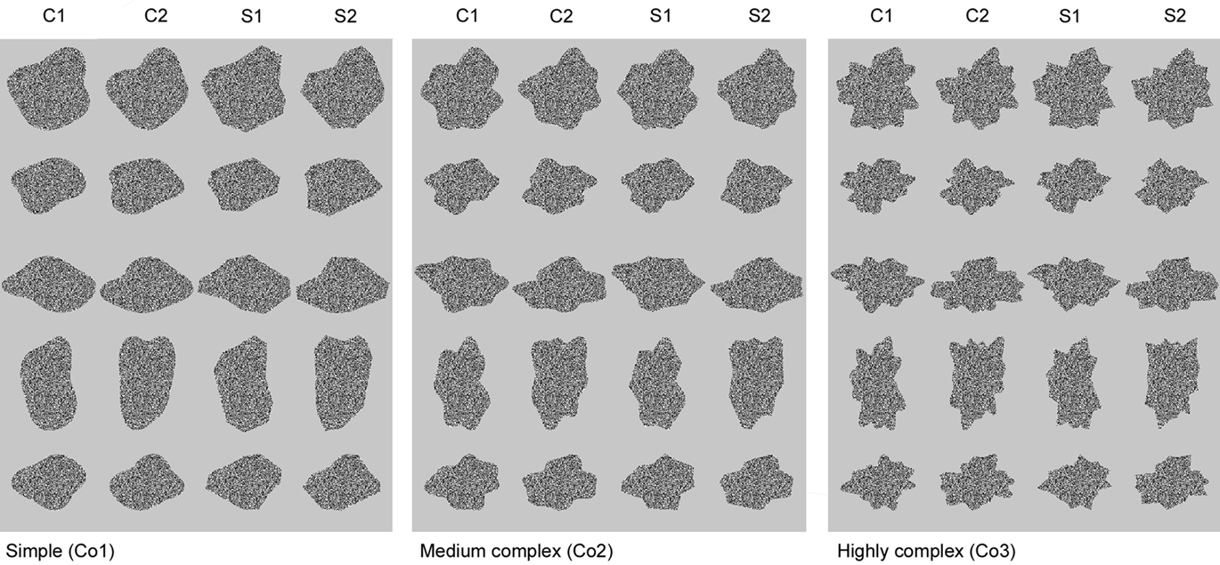
Figure 1. Stimulus set used in Experiment 1. The set is subdivided in three groups of 20 shapes that are approximately equal in complexity; Co1, Co2 and Co3, with increasing numbers denoting increasing complexity. The rows contain five calibrated sets of shapes that can be used to compare neural sensitivity to either changes in the phase of the FBDs or the presence of curved versus straight contours, as a function of complexity. The shapes in columns C1 and C2 are curved and differ in the phase of their FBDs. The shapes in columns S1 and S2 are created by replacing the curves of the shapes in respectively C1 and C2 with straight lines. Within each series, we measured the sensitivity of IT neurons to changes in the phase of the FBDs by computing the difference in response to the shapes in column C1 and S1 compared to the shapes in column C2 and S2, respectively. And we measured the sensitivity of IT neurons to the presence versus absence of curvature by computing the difference in response to the shapes in column C1 and C2 compared to the shapes in column S1 and S2, respectively.

It should be noted that no significantly higher neural sensitivity for simple versus complex FBD-based shapes regarding differences in phase of the FBDs was found in the Kayaert et al. (2005a) study. However, that study was not specifically designed to assess differences in sensitivity to phase changes in low versus high complexity FBD-based shapes and a possible effect in this study could have been masked by several factors. The differences between the complex shapes were larger physically (pixel-wise) than the differences between the simple shapes. The complex shapes contained (at least in some cases) more salient features than the simple shapes, because the amplitude of their FBDs could be higher. Also, the complex shapes could differ in the number and/or frequency of the FBDs as well as in their phase, and in one case differed even in global orientation, while the simple shapes only differed in phase of the FBDs.

We manipulated complexity through the number of concavities and convexities of the shapes, an image property that correlates with most if not all definitions of complexity (e.g., Attneave, 1954; Leeuwenberg, 1969; Zusne, 1970; Chipman, 1977; Hatfield and Epstein, 1985; Richards and Hoffman, 1985; De Winter and Wagemans, 2004). We increased the number of concavities and convexities of the shapes by increasing the number and frequency of the FBDs. The simple shapes were used as a basis to create the more complex shapes (see Materials and Methods) thereby ensuring that the shapes in the different complexity levels are as related to each other as possible (see Materials and Methods for details on stimulus creation).

We calibrated the physical differences between the members of the shape pairs using the Euclidean distance between pixel gray-levels (see Materials and Methods). The physical distance between shapes, defined this way, determines to a large extent visual sensitivity to the shape change and is therefore often used as a null hypothesis against which more specific perceptual hypotheses can be tested (e.g., Cutzu and Edelman, 1998; Grill-Spector et al., 1999; Op de Beeck et al., 2001, 2003; Vogels et al., 2001; James et al., 2002; Vuilleumier et al., 2002; Kayaert et al., 2003, 2005a,b; Kayaert and Wagemans, 2009).

In addition to the pixel-based calibration, we computed similarities among the stimuli using two models of visual processing. The first model, using wavelet-based filters, is an adapted version of the model described in Lades et al. (1993; see Materials and Methods). This model imitates columns of complex V1-neurons, and therefore, to the extent that V1-like properties are preserved in IT, the representation of the shape differences by this model is expected to resemble the neural sensitivities more than the pixel-based differences.

Secondly, we will compare our neural modulations with the Euclidean distances between the C2-units of the HMAX model (described in Riesenhuber and Poggio, 1999 and downloaded from http://www.ai.mit.edu/people/max/ on July 9, 2003). The first layer of HMAX is closely related to the Lades model but the following layer (C2) is designed to extract features from objects, irrespective of size, position and their relative geometry in the image, and is hypothesized to correspond to either V4 or TEO neurons. So, we might expect a closer qualitative and quantitative relationship of the HMAX model with the neural modulations compared to the Lades model.

In Experiment 2, we partially replicate the results of Experiment 1, using different but similar stimuli and two rather than three complexity levels. The stimulus set is presented in Figure 2. In this experiment, the stimuli are presented in two sizes; they can either be the same size as in Experiment 1, or they can be twice as large. Thus, the line segments of the large complex shapes are on average as long as the line segments of the small simple shapes. This allows us to check to which degree an effect of complexity can be attributed to the length of the line segments of the shapes.

FIGURE 2

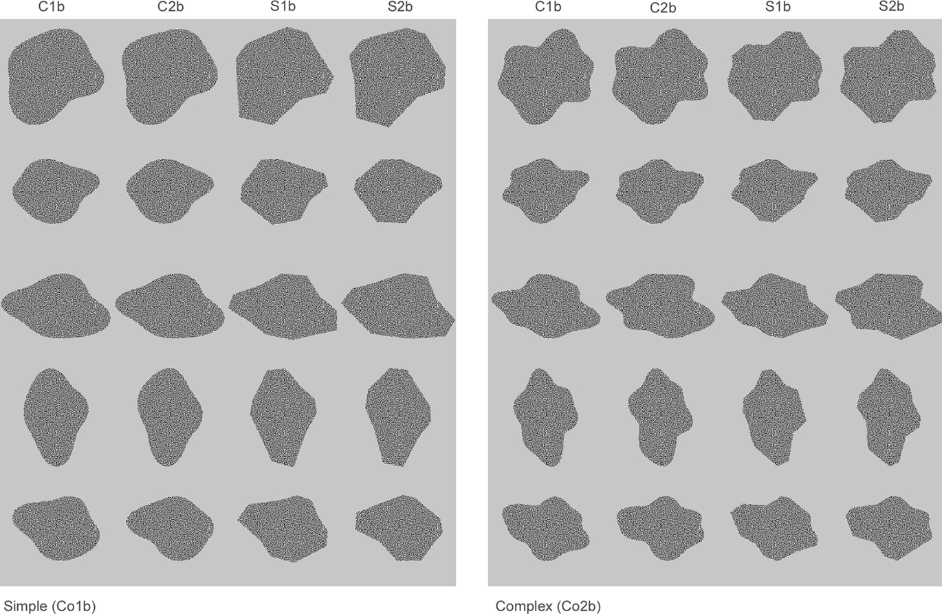
Figure 2. Stimulus set used in Experiment 2. The set contains two groups differing in complexity; Co1b and Co2b (roughly corresponding in complexity with the shapes in Co1 and Co2 of the stimulus set in Figure 1). The rows contain five calibrated sets of shapes that can be used to compare neural sensitivity to either changes in the phase of the FBDs or the presence of curved versus straight contours, as a function of complexity. The shapes in columns C1b and C2b are curved and differ in the phase of their FBDs. The shapes in columns S1b and S2b are created by replacing the curves of the shapes in respectively C1b and C2b with straight lines. We used small and large versions of each of the stimuli, and during the recordings the set was divided in two subsets: 1 containing the first three rows of the global set and 1 containing the two last rows.

Materials and Methods

Single Cell Registrations

Subjects

Two male rhesus monkeys served as subjects. Before conducting the experiments, a head post for head fixation was implanted, under Isoflurane anesthesia and strict aseptic conditions. In addition, we implanted a scleral search coil in one monkey. After training in the fixation task, we stereotactically implanted a plastic recording chamber using coordinates based on anatomical MRIs of each monkey. The recording chambers were positioned dorsal to IT, allowing a vertical approach, as described by Janssen et al. (2000). During the course of the recordings, we obtained in each monkey anatomical MRI scans and CT scans with the guiding tube in situ. This, together with depth ratings of the white and gray matter transitions and of the skull basis during the recordings, allowed reconstruction of the recording positions before the animals were sacrificed. All surgical procedures and animal care was in accordance with the guidelines of NIH and of the K.U. Leuven Medical School.

Apparatus

The apparatus was similar to that described by Vogels et al. (2001). The animal was seated in a primate chair, facing a computer monitor (Panasonic PanaSync/ProP110i, 21 inch display) on which the stimuli were displayed. The head of the animal was fixed and eye movements were recorded using either the magnetic search coil technique or the non-invasive, infrared video-based ISCAN eye position measurement device. Stimulus presentation and the behavioral task were under control of a computer, which also displayed the eye movements. A Narishige microdrive, which was mounted firmly on the recording chamber, lowered a tungsten microelectrode (1–3 Mohm; Frederick Hair) through a guiding tube. The latter tube was guided using a Crist grid that was attached to the microdrive. The signals of the electrode were amplified and filtered, using standard single cell recording equipment. Single units were isolated on line using template-matching software (SPS). The timing of the single units and the stimulus and behavioral events were stored with 1 ms resolution by a PC for later offline analysis. The PC also showed raster displays and histograms of the spikes and other events that were sorted by stimulus.

Fixation task and recording

The monkey was placed in front of the display, at a distance of 75 cm. Trials started with the onset of a small fixation target at the display’s center on which the monkey was required to fixate. After a fixation period of 300 ms, the fixation target was replaced by a stimulus for 200 ms, also shown at the center of the screen. If the monkey’s gaze remained within a 1.5–2° fixation window, the stimulus was replaced again by the fixation spot, and the monkey was rewarded with a drop of apple juice. When the monkey failed to maintain fixation, the trial was aborted and the stimulus was presented during one of the subsequent fixation periods. As long as the monkey was fixating, stimuli were presented with an interval of approximately 1 s. Fixation breaks were followed by a 1-s time-out period before the fixation target was shown again.

Responsive neurons were searched while presenting the stimuli of one of the stimulus sets. All stimuli of this set were shown randomly interleaved. The number of interleaved presentations of a given shape was at least 4 for a given neuron (median number of presentations per stimulus: 12).

Stimuli

The stimuli we used are made using a FBD formalization of shape, in which the shape boundary function is expanded in a Fourier series. This kind of shapes has been used in several studies on IT neural selectivity (Schwartz et al., 1983; Op de Beeck et al., 2001; Kayaert et al., 2005b; De Baene et al., 2007). Each shape can be fully described by its set of FBDs which can differ in phase, frequency, and amplitude. We manipulated the frequency of the FBDs to create shapes of different complexity, and we varied the phase of the FBDs to vary the general shape of the different stimuli. One can also manipulate the amplitude of the FBDs, which would result in more pronounced indentations but we did not do this in this study; all FBDs had the same amplitude. We did, however, manipulate the presence of curvature in the contour by replacing the curves in the contour by straight sides. For this, the line-endings were handpicked (in Photoshop 5.5), after which their exact position was optimized to minimize the physical distance with the curved shapes (with physical distance defined as the Euclidean distance between the pixels, like our other calibrations, see further in the Section “Materials and Methods”). The optimization was done using a custom made program in MATLAB, version 5.3.

All stimuli were filled with a random noise-pattern, consisting of black and white dots, as in Op de Beeck et al. (2001). We incorporated the restriction that the number of black and white dots should be equal for 2 × 2 squares in the texture, so the textures were highly uniform. All stimuli were made using MATLAB, version 5.3. Stimuli were presented on a gray background. The background had a mean luminance of 6.4 cd/m² and the black and white pixels a luminance of 0 and 20 cd/m², respectively. Stimuli were shown at the center of the screen.

Experiment 1

The stimuli used in Experiment 1 are presented in Figure 1. The set consisted of 60 shapes, created by means of different FBDs. The shapes extended approximately five visual degrees (with considerable variance between the shapes). They are subdivided in three groups of increasing complexity (Figure 1). The groups will be called simple, medium complex, and highly complex shapes in the text and denoted Co1, Co2, and Co3 in the figures. Each group consists of 10 shapes that are approximately equal in complexity. The stimuli in the medium and highly complex shape groups were created by adding higher frequency FBDs to the stimuli in the simple and the medium complex shape groups, respectively. The number of the FBDs in the different complexity groups was respectively 4, 5, and 6, and their frequencies were respectively [1;2;3;4], [1;2;3;4;7], and [1;2;3;4;7;11].

Each of the five rows in each complexity group (Figure 1) consists of four shapes that are matched in size and aspect-ratio. The first two stimuli (columns C1 and C2) differ in the phase of their FBDs, thus creating differences in the configuration of the curves. The next two stimuli (columns S1 and S2) were created by replacing the curves of the shapes in C1 and C2, respectively, with straight lines, thereby taking care to preserve the general shape of the stimuli. Hence, the differences between the stimuli in S1 and S2 are also configurational differences but now between stimuli with straight contours. But the difference between the stimuli in C1 and S1 and the stimuli in C2 and S2 is the presence of curved or straight edges, respectively.

Thus, each complexity group has 5 pairs of curved shapes differing in the configuration of their features (“C1” versus “C2”), 5 pairs of straight shapes also differing in the configuration of their features (“S1” versus “S2”), and 10 pairs of shapes that differ by having either curved or straight contours (“C1” versus “S1” and “C2” versus “S2”).

Experiment 2

Figure 2 shows the collection of stimuli that were used in the second experiment. It was made in a completely analogous fashion as the stimuli in Figure 1 but contains only two complexity groups. The number of FBDs in the different complexity groups was respectively 4 and 5, and their frequencies were respectively [1;2;3;4] and [1;2;3;4;6]. In order to examine the influence of size, each stimulus was shown in two versions; one that was roughly the same size as the stimuli in Figure 1 (extending ±5°) and one that was twice as large (extending ±10°). Thus, in total, this second collection comprised 80 stimuli. This is a large set to record from single neurons, as we can only record from a particular neuron for a limited amount of time. Thus, in order to increase the number of presentations within each individual neuron, we divided the stimuli in two subsets: the first (sub)set contained the first three rows and the second (sub)set contained the last two rows.

Number of Image Features

Adding higher frequency FBDs to the more complex shapes resulted in an increase in the number of concavities and convexities in the curved shapes and an increase in the number of corners in the straight shapes. This was quantified by instructing 10 naïve subjects to mark either the convexities and concavities or the corners on print-outs of the stimuli (size: 6.4 cm × 6.4 cm). Both the average and the median correlation between subjects (over stimuli) of the number of items marked was 0.98. The number of features was defined as the median number of items marked by the subjects. The average number of features of the shapes in the first stimulus set (Figure 1) was 8, 14, and 21, for the simple, medium and highly complex shapes, respectively. Regarding the stimuli of the other two sets (Figure 2), the numbers were 8 and 13 for the simple and complex shapes, respectively.

Image-Similarity Measures

Pixel-based differences

We calibrated the physical differences between the members of the shape pairs using the Euclidean distance between pixel gray-levels. Throughout all complexity levels, the physical differences were much smaller for the shape pairs where the members differ in the presence versus absence of curvature than for the shape pairs where the members differ in phase of the FBDs. The physical difference within the pairs becomes slightly larger as shape complexity increases. Therefore, any higher sensitivity to simple shapes must originate in the visual system and cannot be due to physical differences.

All the following calibrations were done on the silhouettes of the stimuli, i.e., without the random noise filling. We computed the Euclidean distance between the gray-level values of the pixels of the images as follows: with G¹ and G² the gray levels for picture 1 and 2 and n the number of pixels. The Euclidean distances presented in the result section were computed with position-correction. For instance, we computed the Euclidean distance for 99 by 99 different relative positions of the stimuli (maximum position shift: 50 pixels or 14% of the images), and then withheld the smallest value. We also did a calibration without position-correction, and because some neurons might be mainly sensitive to low spatial frequencies, we performed a low-pass filtering on the images using convolutions with Gaussian filters with a standard deviation of either 8 or 15 arc’.

The pixel-based differences for the different calibrated comparisons between shapes are presented in Figure 3B for Experiment 1 and in Figure 9C for Experiment 2. The differences were much smaller for the shapes differing in the presence versus absence of curvature than for the shapes differing in phase of the FBDs. We also made sure that on average the pixel difference increased as the complexity increased for each kind of shape difference and this for all our measurements (i.e., the position-corrected and the ordinary measurements, the latter on the normal as well as on the filtered images). There was no tendency for the differences between the complex shapes to become relatively smaller with low-pass filtering.

FIGURE 3

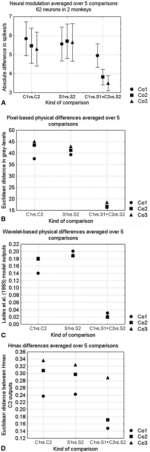
Figure 3. (A) Neural sensitivities for the different kinds of shape differences. The kind of shape difference is presented on the abscissa using the column notations of Figure 1 (respectively shape differences within curved shapes, shape differences within straight shapes and curved versus straight contours) while the complexity of the stimuli is represented by circles, squares, and triangles for shapes from respectively Co1, Co2, and Co3. Curved versus straight comparisons were first averaged within the rows (according to the formula (C1 − S1| + |C2 − S2|)/2), thus also their standard errors are on five data points. Vertical bars denote standard errors. (B) Pixel-based dissimilarities, (C) Lades model dissimilarities, and (D) Euclidean distance between HMAX C2-layer outputs.

Wavelet-based filters

The first model, using wavelet-based filters, is an adapted version of the model described in Lades et al. (1993). The Lades et al. (1993) model produces wavelet-based image measures. It filters the images using a grid of Gabor jets and then computes the difference between the outputs of the different Gabor jets for the images of a pair. In the present implementation, the square grid consisted of 10 × 10 nodes with a node approximately every 10 pixels, horizontally and vertically, as the images are rescaled to be squares of 128 pixels (instead of the original 350 pixels). Each Gabor jet consists of 40 Gabor filters. They can have five possible spatial frequencies which are logarithmically scaled. The lowest spatial frequency filter covers a quarter of the image while the highest-frequency filter covers about 4 pixels on each side. They can have eight possible orientations. At each node, a Gabor jet can be described as a vector of 40 Gabor filter outputs. The similarity of a pair of images is computed as an average of local similarities between corresponding Gabor jets. The local similarity is given by the cosine of the two vectors, thereby discarding phase parts. The grids were positioned on the stimuli in such a way as to maximize similarity between pairs of images. We used Lades model dissimilarities in order to facilitate comparison with the neural distances. The former dissimilarities are computed by subtracting the Lades model similarities from 1. Figure 3C shows the Lades dissimilarities for the complexity groups depicted in Figure 1.

HMAX C2 layer outputs

We computed the Euclidean distances between the outputs of C2-units of the HMAX model (described in Riesenhuber and Poggio, 1999 and downloaded from http://www.ai.mit.edu/people/max/ on July 9, 2003). This hierarchical, feature-based model consists of five layers. The units of the first four layers show a greater degree of position and size invariance and respond to increasingly more complex features at hierarchically higher layers. The fifth layer consists of units that are made to respond optimally to particular views of particular objects. We computed the similarity between the shapes using the output of the fourth, C2 layer. These units are designed to extract moderately complex features from objects, irrespective of size, position, and their relative geometry in the image, and are hypothesized to correspond to either V4 or TEO neurons (see Riesenhuber and Poggio, 1999 for more details). Image similarity was computed as the Euclidean distance between the outputs of the 256 C2 units. Figure 3D shows the Euclidean distances between HMAX C2 outputs for the complexity groups depicted in Figure 1.

Analyses

Since the reported effects in this study were mirrored in the data of both monkeys, we presented our data pooled across monkeys.

The response of a neuron was defined as the number of spikes during a time interval of 250 ms, starting from 40 to 120 ms after stimulus onset. The starting point of the time interval was chosen independently for each neuron to best capture its response, by inspecting the peristimulus time histograms, but was fixed for a particular neuron. Each neuron showed significant response modulation to the stimulus set, which was tested by an ANOVA.

The degree of response modulation to each possible stimulus pair was assessed by calculating the normalized Euclidean distance between the response over each of the 119 neurons, using the following formula: with the average response of neuron i to stimulus 1 and n the number of neurons. The resulting distance matrix allowed inferences as to the representation of the shapes of the different stimulus sets in IT. We obtained similar results when we used a distance matrix based on the normalized responses of the neurons. The responses of each neuron were normalized by dividing the average response to a stimulus by the maximum average response of that neuron across the different stimuli.

We used non-parametric statistical tests to compare response modulations to different stimulus pairs.

Multidimensional scaling-analyses

Multidimensional scaling (MDS) analyses were done using Statistica software (StatSoft, Tulsa, OK, USA). We employed the standard non-metric MDS-algorithm (Shepard, 1980) using a matrix of the distances between each pair of shapes as input. The distances were computed using either neural modulations [Euclidean distance (see above); same procedure as Young and Yamane, 1992; Op de Beeck et al., 2001; Vogels et al., 2001; Kayaert et al., 2005a; De Baene et al., 2007), or the different image-similarity measures (see above). The MDS-algorithm will arrange the stimuli in a low-dimensional space while trying to maintain the observed distances. This low-dimensional configuration can be freely translated, scaled, and rotated.

We used MDS analyses to visualize the representation of the shapes in our stimulus sets, but also to establish the degree to which the neurons and the image measurements can separate the shapes according to a particular shape property, e.g., complexity, curved versus straight edges, etc. The amount of separation was operationalized as the amount to which we could, based on the neural data, separate two groups of shapes that differ in their value on the shape property under investigation. So, we attempted to separate the curved from the straight shapes, the low complexity from the moderate complexity shapes, the moderate complexity from the high complexity shapes, etc. This was done by rotating the MDS-solution in such a way to find a maximum separation between the groups under investigation along one of the dimensions.

This was done in two steps. First, we determined the number of dimensions we would use to explore the responses to the stimulus groups under investigation. We based our decision on visual inspection of the scree plot and took care to choose a manageable number of dimensions that would still explain most of the variance in the data (the exact number depending on the stimuli under investigation, but fluctuating around 90%). Secondly, we rotated the resulting MDS-solution in such a way to find a maximum separation between the groups under investigation along one of the dimensions. The rotation was done systematically using a custom written Matlab algorithm. It orthogonally rotates the configurations in steps of 1° and at each step calculates the overlap between the members of the groups along each dimension. Finally, it withholds the rotation at which the overlap between the members of groups along one of the dimensions was the smallest. Within this final low-dimensional solution, one can easily determine along which of the dimensions the groups are best separated.

We used randomization statistics to assess whether the separations we found were significantly different from those obtained from a random configuration of two sets of an equal number of points without a priori separation. We used two complementary randomizations to do this. In a first randomization, we randomized the stimulus labels within the MDS-solution. Thus, the points were arbitrarily divided in two groups, and this was repeated 1000 times. Thus, we could assess the odds of a complete separation (or a separation with equal or less mismatches as present in the data) given a certain configuration of neural or model distances, but based on random group membership. The expected separations and the p-values presented in the result section are based on these randomizations.

We also did a complementary randomization test in which we randomized the neural responses of each neuron separately over all stimuli, before doing MDS. This results in a completely random configuration, and all reported effects were equally significant using this randomization. Also the latter randomization was repeated 1000 times and we computed the proportion of random configurations that yielded a separation at least as great as the separation under testing. The test was significant when the latter proportion was smaller than 0.05.

Results

During Experiment 1, we recorded the responses of 62 anterior TE neurons from two monkeys (32 in monkey 1 and 30 in monkey 2) that showed significant modulation to the stimuli presented in Figure 1 (ANOVA, p < 0.05). Their average firing rate was 24 spikes/s for the shapes in the simple group and 23 spikes/s for the shapes in both the medium and high complexity groups. Table 1 gives some further response characteristics of the neurons.

TABLE 1

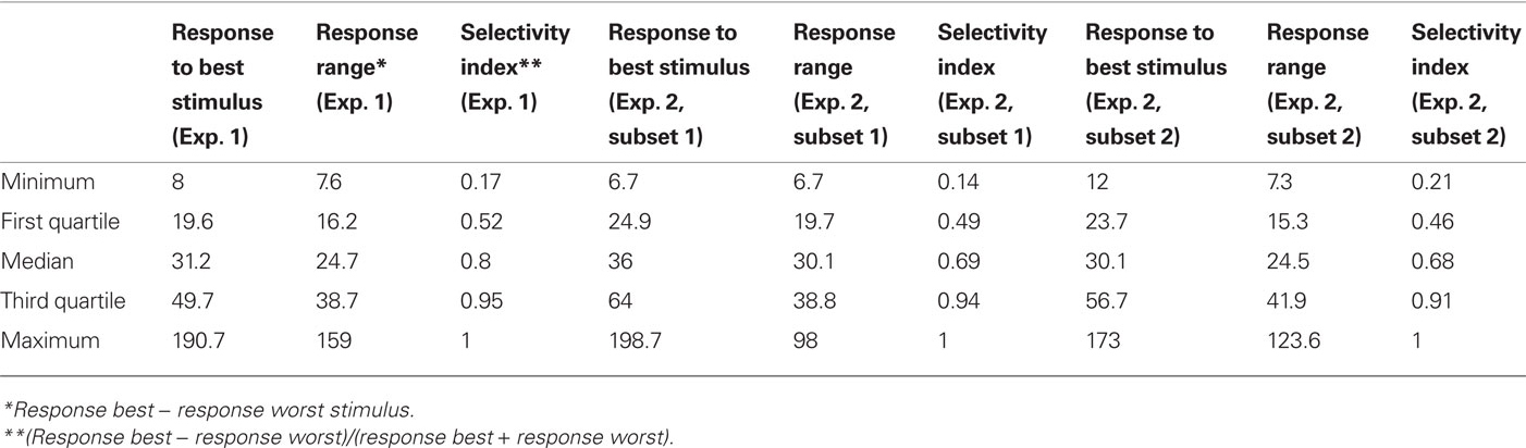
Table 1. Distribution of some neural response characteristics, in spikes/s.

Figure 4 shows examples of some of the neurons we recorded. Figures 4A and 5B are examples of neurons that were selective to both a particular level of complexity, and the shape variations within this level. The neuron in Figure 4A was highly selective and responsive to shape variations in the simple shapes, responding much less to the shape variations in complex shapes. And in each group the average response was strongest for the straight shape. The neuron in Figure 4B preferred some of the highly complex shapes but also responded slightly to the medium complex shapes, and there was no response to the simple shapes. The neuron in Figure 4C was mainly tuned to the global shape of a stimulus, preferring the stimuli in the third row of Figure 1. The neuron in Figure 4D was tuned to curvature, preferring curved over straight shapes. However, also these latter two neurons could be used to represent complexity, as the maximum response within each complexity group decreased as complexity increases. Thus, complexity was represented by these neurons, but it was done so orthogonal to shape representation, with both variables intermingled in individual neurons.

FIGURE 4

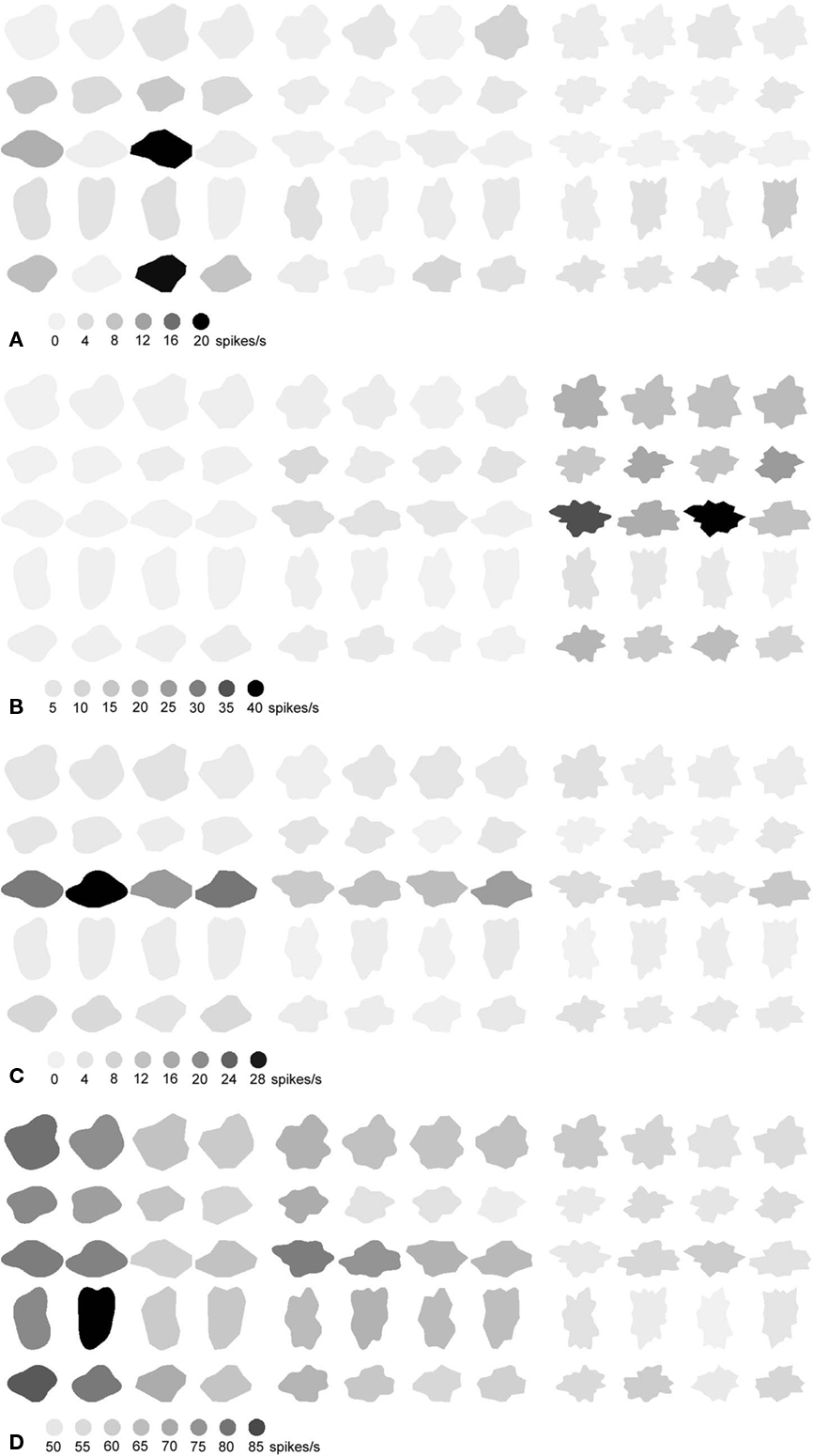
Figure 4. Responses of five neurons (A–D) to the stimulus set in Figure 1. The darker the depiction of the shapes, the stronger the response. The calibration bars underneath each of the sets indicate the response (in spikes/s) corresponding to the different shades.

Categorical Representation of Simple Versus Complex Shapes

In order to disentangle the influence of complexity from other shape sensitivities and to analyze the data on a population level, we conducted an MDS analysis on the Euclidean distances (see Materials and Methods for formula) between the neural responses to the stimuli in Figure 1. The number of dimensions had to be modest to make the solution interpretable. We used a 2-D solution, because this already included the dimension of interest (e.g., a dimension that segregates the stimuli according to membership of the complexity groups) and higher-dimensional solutions did not yield more insight in the data. We do not claim that the response pattern of our neural population is necessarily 2-D in nature; the “real” number of dimensions would correspond to the number of independent stimulus characteristics the different neurons extract, and this is certainly higher. Nevertheless, the observed modulations to the stimulus pairs (the neural distances) were well preserved within the low-dimensional space (explained variance of 2-D solution: r² = 0.86).

The MDS-solution is presented in Figure 5A. The circles represent simple shapes, the squares medium complex shapes and the triangles highly complex shapes. The numbers at each data point refer to the rows within each group in Figure 1. The first dimension (shown on the horizontal axis) is probably related to the global shape of the stimuli, as it separates the vertically oriented stimuli in row 4 from the other, more horizontally oriented stimuli. The second dimension (shown on the vertical axis) ranks the stimuli according to their complexity group. The simple shapes were roughly separated from the complex shapes. However, there was no segregation between the medium and highly complex shapes, and we did not find such a segregation in any dimension in a higher-dimensional solution (up to four dimensions) either. The segregation (with merely two shapes situated on the “wrong” side of the border) between the simple and complex shapes was higher than what would be expected based on a random configuration (p < 0.001, randomization statistics). Thus, within this low-dimensional MDS-solution, IT neurons can differentiate the simple from the medium complex shapes but not the medium from the highly complex shapes.

FIGURE 5

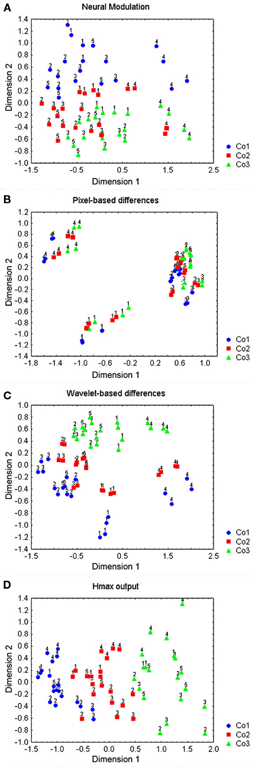
Figure 5. Two-dimensional MDS-solutions for the shapes represented in Figure 1. The circles represent simple shapes, the squares medium complex shapes and the triangles highly complex shapes. The numbers at each data point indicate to which row in Figure 1 the shape belongs. (A) Solution for the neural Euclidean distances, (B) solution for the pixel-based distances, (C) solution for the wavelet-based distances, and (D) solution for the HMAX C2-layer distances.

Comparisons of the neural representation of complexity with different models

We compared the neural representation of our shapes to a hypothetical representation that faithfully reflects the physical overlap between the stimuli (i.e., the pixel-based differences, see Materials and Methods). We choose a 2-D solution for this pixel-based representation. The explained variance of the MDS-solution was 0.92, even higher than that of the neural solution. Adding more dimensions to the model resulted in a small decrease in stress but the scree plot pointed to a 2-D solution. None of the possible higher dimensions showed a shape ranking that might be related to complexity. The position of the stimuli in the 2-D space is presented in Figure 5B. The stimuli were segregated according to their global shape, with the stimuli in row 1 and 4 being segregated from each other and from the stimuli in the other rows. The absence of a segregation of the shapes according to their complexity in the pixel-based configuration demonstrates that the representation of complexity in the neural data is not merely a faithful reflection of the physical differences between the stimuli but indicates further processing specifically related to the complexity levels of our stimuli.

We also compared our representation with that of two models designed to mimic neural responses, i.e., a wavelet-based model (Lades et al., 1993) and the Euclidean distances between the C2-units of the HMAX model (Riesenhuber and Poggio, 1999; see Materials and Methods for the implementation of both models). Figures 5C and 5D represent the 2-D MDS-solutions of the wavelet-based and HMAX model distances. The explained variances were 90 and 96% for the wavelet-based model and HMAX respectively. In agreement with the neural data, one dimension can be seen as encoding global shape In accordance with the neural data the shapes in row 4 were best segregated from the others, especially using the wavelet filters that in this respect seemed to be more related to the pixel-based differences.

Also in agreement with the neural data, the second dimension in both models represented the differences in complexity between the stimuli. However, the better separation of the simple versus medium complex compared to the medium versus highly complex shapes found in the neural data was completely absent. Both models roughly separated the simple from the medium complex shapes (HMAX has 4 errors and the wavelet-based model has 10, but to the defense of the latter it must be said that it roughly preserves the ranking within the different series) but they separated the medium complex shapes even better from the highly complex shapes (complete separation in HMAX and two errors in Lades).

The Effect of Complexity on the Sensitivity for Shape Changes

Modulation to shape pairs differing in either presence of curvature or phase of the FBDs

We could use the responses of the neurons to the shape pairs within this stimulus set to measure the neural sensitivity for the phase of the FBD’s as well as for the presence of curved versus straight edges, and this as a function of the complexity of the shapes. The neural sensitivities are presented in Figure 3A. There was no influence of complexity on the modulation to configurational shape differences, but there was a significant influence on the modulation to absence versus presence of curvature (with higher modulation in the simple than in the complex shapes, Wilcoxon matched pairs test, p < 0.02 in both cases, over all curved versus straight comparisons, n = 10). This was illustrated by the neuron in Figure 4D, which responded more to curved compared to straight shapes, but only for the simple shapes.

Sensitivity to presence of curvature as a dimension in shape space

This was assessed by doing an MDS analysis within each of the three complexity groups separately. The solutions were 3-D and explained 94, 96, and 98% of the variance, respectively. In each case, we rotated the 3-D space so that one of the dimensions separated the curved and the straight shapes with as little errors as possible. The solutions are shown in Figure 6. There was a separation within the simple shape group, with the number of errors (1) significantly lower than chance (p < 0.02), but not within the complex shape groups where the number of errors (5 and 4, respectively) did not lie significantly underneath the four errors expected by chance (p > 0.05).

FIGURE 6

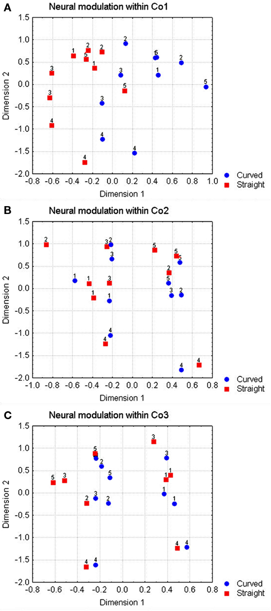
Figure 6. Representation of two dimensions of a 3-D MDS-solution for the shapes within each complexity group of Figure 1, using the neural Euclidean distances. Circles indicate curved shapes, squares indicate straight shapes. The horizontal axis shows the dimension that best separates the curved from the straight shapes. (A–C) Contain the solutions for complexity groups 1–3.

Sensitivity to the presence of curvature in the medium and highly complex shapes

The effect of complexity on the modulation to straight versus curved contours was confined to the transition between simple and medium complex shapes. In order to establish whether the neurons could still detect the differences between the curved and the straight shapes at the second level of complexity, we determined the number of times a neuron responds significantly differently to the curved compared to the straight shape (t-test, p < 0.05), relative to the total number of curved versus straight shape pairs. This proportion was calculated for each complexity group separately, including in the analyses only those neurons that modulated significantly to the shape changes in general (ANOVA, p < 0.05; note that most shape changes were by far larger than the curvature differences, which resulted in a large probability that a neuron would only be selective to a shape change not involving curvature difference). The proportions were 37, 17, and 15% for the simple, medium and highly complex shapes, respectively; all significantly different from 5% (according to the binomial distribution, p < 0.05, n = 550, 540, and 520, respectively).

In this context, it should be noted that the differences between the curved and straight stimuli, although subtle on paper, were perfectly visible on our monitor.

Influence of complexity on the shape sensitivity of the different models

The model distances on the calibrated shape pairs are shown in Figures 3B–D, in a similar fashion as the neural distances in Figure 3A. As is expected from the calibration, the pixel-based distances (Figure 3B) were smaller for the difference between curved and straight edges than for the global shape changes, and generally slightly increased with increasing complexity. The wavelet-based model (Lades et al., 1993; Figure 3C) was best related to the neural data, as there is a slightly higher sensitivity to curvature differences for the simple shapes. HMAX however showed an increase in sensitivity with higher complexity, in accordance with the pixel data but opposite to the neural data (Figure 3D).

Also for the model distances, we performed MDS analyses within each of the three complexity groups separately. There was no separation whatsoever in any of the pixel-based configurations (errors are 7, 6, and 6 for the three complexity groups, respectively; explained variances are 79, 72, and 72%¹). Within the pixel-based MDS-solutions, the curved and the corresponding straight shapes were actually placed upon each other as the pixel-differences between curved and straight were extremely small compared to the shape differences.

In accordance with the pixel distances and contrary to the neural data, 3-D MDS-solutions of the Lades and HMAX models on the simple shapes (explained variance twice 98%) yielded no linear separation between curved and straight whatsoever (both six errors which is above the four errors expected by chance).

Experiment 2: Replicating the Effect of Complexity on Neural Sensitivity for Stimuli Extending 5 and 10 Visual Degrees

We wanted to see whether the effects of complexity would also hold for a stimulus set in which the line segments for the complex shapes were as long as for the simple shapes we used in our first physiological experiment, so we replicated the experiment for stimuli extending 5 and 10 visual degrees. To this means, we created a second stimulus set, presented in Figure 2 (see Materials and Methods). We recorded the responses of 55 (31 in monkey 1 and 24 in monkey 2) and 52 (30 in monkey 1 and 22 in monkey 2) anterior TE neurons for each subset, respectively. Table 1 gives some response characteristics of the neurons.

We performed an MDS on both subsets of neurons to get a global idea of how the neurons represented the dimensions within the subset. The number of dimensions (4 and 3) was chosen based on the scree plot and was sufficient to explain 96 and 98% of the variance. The solutions are presented in Figures 7A,B for the subset containing the first three rows of the global stimulus set and in Figures 7C,D for the subset containing the last two rows of the global stimulus set. The dimensions in these solutions could perfectly separate the small from the large stimuli. They could reasonably well separate the simple from the complex shapes with two and three errors, respectively (p < 0.01, randomization statistics). There was also a certain amount of curvature encoding (with the curved version of a shape systematically getting a higher load on the dimension that separates the simple from the complex shapes), which was, however, more ambiguous and only present for the simple shapes.

FIGURE 7

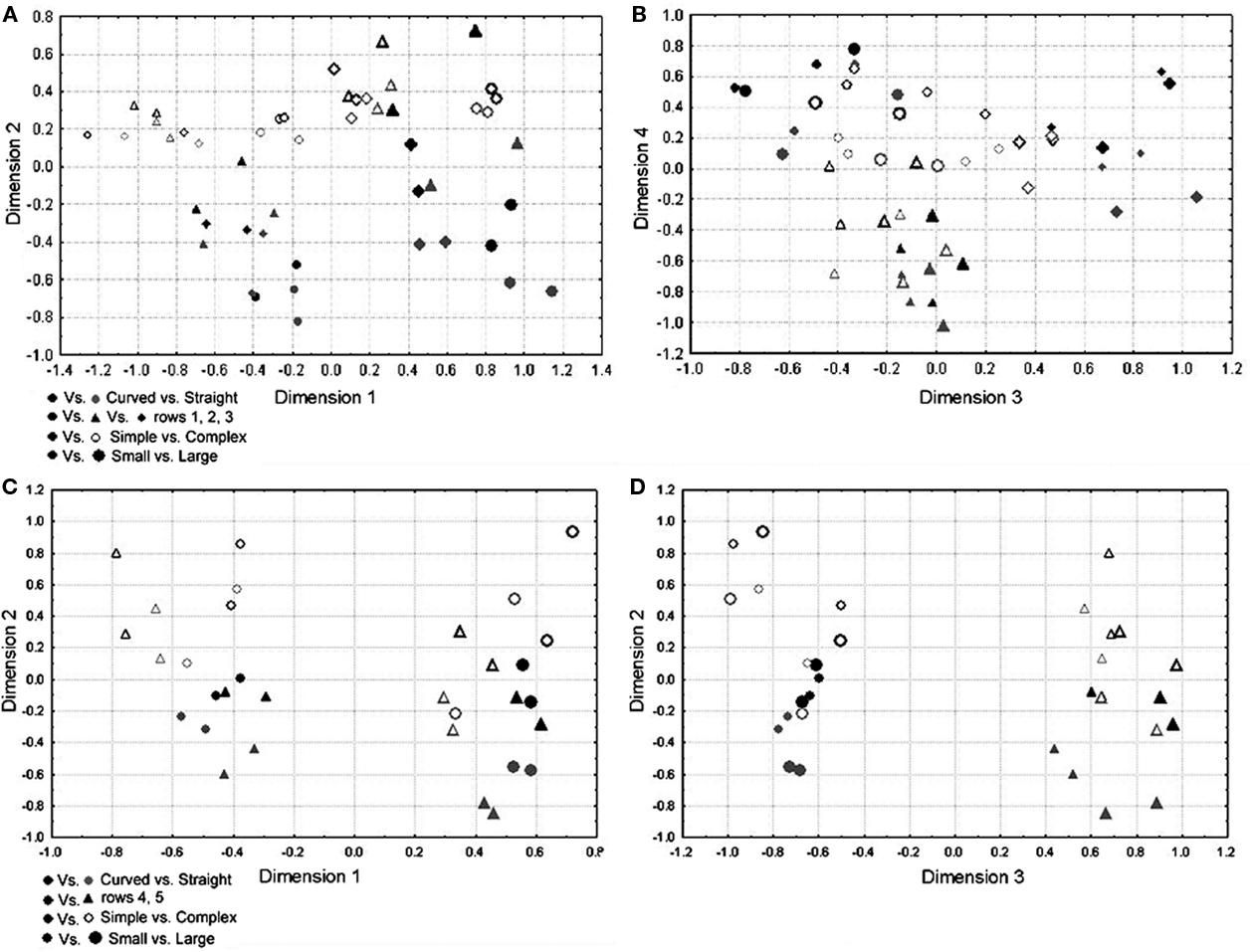
Figure 7. Representations of the MDS-solutions for the subsets of shapes used in Experiment 2. Curved shapes are presented in black, straight shapes in gray; simple shapes are denoted by filled symbols, complex shapes by open symbols; larger shapes are presented by larger symbols; the row of the shape in Figure 2 is represented through the shape of the symbol (see legend). (A,B) The four dimensions of the solution for subset 1 (first three rows in Figure 2), (C,D) the three dimensions of the solution for subset 2 (last two rows in Figure 2).

This global representation was reflected by the individual neurons shown in Figure 8. The neuron in Figure 8A was mainly performing complexity encoding, with a consistently higher response to the complex compared to the simple stimuli. The same neuron was also very sensitive to size. Regarding the same subset, the neuron in Figure 8B encoded curved versus straight, but only for the simple shapes. The neuron in Figure 8C was recorded using the second subset and behaved similarly as the neuron in Figure 8B, only this one extended the curvature encoding to the complex shapes, albeit to a lesser degree. In both Figures 8B,C, the preference for either curved or straight shapes was preserved over shape variations.

FIGURE 8

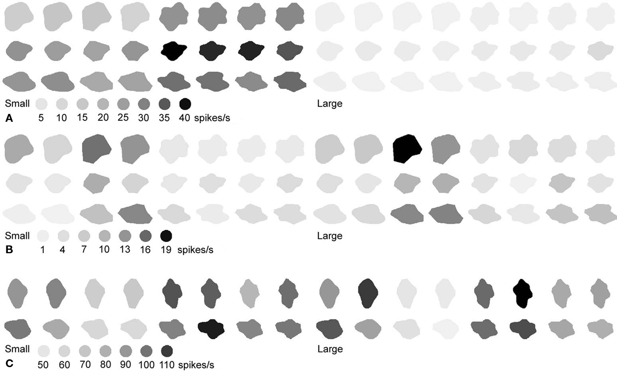
Figure 8. Responses of three neurons (A–C) to shapes from the set of Figure 2. The calibration bars underneath each of the sets indicate the response (in spikes/s.) corresponding to the different shades. The responses to the shapes on the left depict the responses to the small size versions of the shapes, those to the shapes on the right depict the responses to the large versions of the shapes. (A,B) Show responses to shapes in the first three rows of Figure 2, while (C) shows responses to the shapes in the last two rows of Figure 2.

The effect of complexity on shape sensitivity was similar to the effect obtained in Experiment 1, as is shown in Figure 9A for the small and Figure 9B for the large versions of the shapes for the normalized Euclidean distances, averaged over the comparisons in the rows of Figure 6 (curved versus straight comparisons were first averaged within the rows, thus also their standard errors are on five data points). There was generally no influence of complexity on the modulation to configurational shape differences (p > 0.05, Wilcoxon matched pairs test, for both the straight and the curved shapes and both the large and the small stimuli over all shape pairs, n = 5), but there was a significant influence on the modulation to absence versus presence of curvature (p < 0.05, Wilcoxon matched pairs test, for both the large and the small stimuli, over all curved versus straight comparisons, n = 10).

FIGURE 9

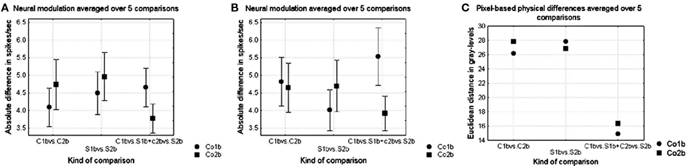
Figure 9. (A,B) Average neural modulation for the different kinds of shape comparisons in Experiment 2. The kind of shape difference is presented on the abscissa using the column notations of Figure 2 (respectively shape differences within curved shapes, shape differences within straight shapes and curved versus straight contours) while the complexity of the shape is represented by the different symbols (circles and squares for shapes from respectively Co1b and Co2b). Curved versus straight comparisons were first averaged within the rows (according to the formula: (|C1 − S1| + |C2 − S2|)/2, thus also their standard errors are on five data points. Vertical bars denote standard errors. (A) Shows the neural modulation for the small size versions of the shapes and (B) the neural modulation for the large versions. (C) Pixel-based dissimilarities for the different kinds of shape comparisons.

In line with the results of Experiment 1, there was a complete separation between curved and straight shapes in the simple groups for subset 1 (small and large stimuli separately, on 3-D solutions, explained variances 81 and 98% respectively, p > 0.05, random configuration resulted in on average two errors) and 2 (small and large stimuli separately, on 2-D solutions, explained variances 92 and 88% respectively, p < 0.05, random configuration resulted in on average one error). However, the corresponding numbers of errors within the complex groups are 2, 1, 0, and 1 for the small and large stimuli of subsets 1 and 2, respectively (also 3- and 2-D solutions, with explained variances of 94, 92, 98, and 98%; not significantly different from chance).

These general effects are illustrated by the neurons in Figures 8B,C, which responded more strongly to the curved and the straight shapes within each series, and this segregation was more pronounced within the simple than within the complex group.

The modulation to differences in size could be very pronounced, as is illustrated by the neuron in Figure 8A. This modulation played an important role in the MDS-solution and the mean absolute difference between the small and the large stimuli was 8 spikes/s. Nevertheless, in general the shape selectivity remained preserved over the size variation, as shown in Figures 10A,B for the first and the second subset, respectively.

FIGURE 10

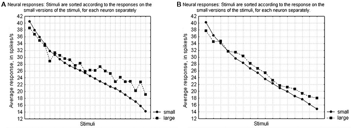
Figure 10. Average preservation of the selectivity of the IT neurons over changes in size. Stimuli are sorted according to the response strengths for the small versions of the stimuli, for each neuron separately, and the average response is shown for either the small versions (circles) or the large versions (squares). (A) For the stimuli in subset 1 (the first three rows of Figure 2). (B) For the stimuli in subset 2 (the last two rows of Figure 2).

Discussion

The present findings agree with those of Kayaert et al. (2005a): the responses of IT neurons can be used to linearly separate simple from more complex shapes. We extend these findings by showing that there is no linear separation possible between shapes of medium and high complexity. Thus, the visual system seems to be more sensitive to the distinction between our simple and complex shapes than to the distinction between different higher levels of complexity.

We found that the higher sensitivity for the distinction between curved and straight contours compared to shape changes within either the curved or straight shape group is only present in simple shapes and not in more complex shapes. Despite the more rigorously controlled stimulus set, which allowed for a better comparison of shape changes within the different complexity groups, there was still no effect of complexity on shape changes within either the curved or straight shape group. The effects in our study could not be predicted from either the physical differences between the shapes or from wavelet-based measures or HMAX C2 layer outputs.

The lack of influence of complexity on the neural sensitivity to changes in the phase of the FBDs is at odds with psychophysical studies measuring a higher sensitivity for shape changes in simple versus complex shapes during (delayed) shape matching (Vanderplas and Garvin, 1959; Pellegrino et al., 1991; Larsen et al., 1999; Kayaert and Wagemans, 2009). This is especially the case for the study of Kayaert and Wagemans (2009), which found the speed and accuracy of delayed shape matching to be inversely correlated with complexity, using the same stimulus set as the current study. One reason for this discrepancy might be a difference in familiarity with the stimuli. The subjects in the Kayaert and Wagemans (2009) study only saw the stimuli during a 1-h experimental session while the monkeys in this study saw the stimuli continuously during the recordings, which could last 3–4 h a day for several weeks. It has been shown in various tasks that the effects of complexity can fade away relatively quickly after training (Vanderplas and Garvin, 1959; Pellegrino et al., 1991; Goldstone, 2000). Training can also lead to a more holistic representation of two-part objects in monkey IT cortex (Baker et al., 2002). Even mere exposure to stimuli causes subjects to bind together different features that occur together, which could enhance the representation of more complex shapes (Fiser and Aslin, 2001; Orbàn et al., 2008).

Our data do show a clear effect of complexity on the detection of curved versus straight shapes. This effect is confined to the transition between simple and medium complex shapes. The curvature change is however still detectable in the highly complex shapes, which excludes a floor effect. Since the contours of the simple shapes contain longer line segments than the contours of the complex shapes, the effect might be related to spatial summation, i.e., the tendency of non-endstopped V1-neurons to fire more strongly as a line becomes longer, up to a certain length (Schiller et al., 1976). However, greatly enlarging the line segments by doubling the size of the shapes, as was done in Experiment 2, did not lift the neural sensitivities of the larger complex shapes to the level of the smaller simple shapes, implying other factors as well.

The detection of the presence versus absence of curvature along the contours of the shapes in our stimulus set demands greater acuity than the detection of the other shape changes. Therefore, our curvature-specific complexity effect, could, irrespective of its origins, be related to studies that find enhanced detectability of the contours of smooth, simple shapes as well as greater acuity along these contours. It is, for instance, easier to detect a contour of Gabor patches when it is part of a closed shape (Kovacs and Julesz, 1993) but only when the contour does not curve too much (Pettet et al., 1998). In general, detection of a closed Gabor contour is negatively affected by the magnitude (Field et al., 1993; Hess and Dakin, 1997; Hess et al., 1998) and the number (Pettet, 1999) of its curves. These effects have also been shown to play a role in more complex shapes (Machilsen and Wagemans, 2011), in Gaborized outlines of everyday objects (Nygård et al., 2009; Sassi et al., 2010), and in fragmented outlines of everyday objects (Panis et al., 2008; Panis and Wagemans, 2009). Moreover, similar results have been found in discrimination studies where the discrimination of small deformations between closed circular contours was enhanced only in contours containing up to about five local curvature extrema (Wilkinson et al., 1998; Loffler et al., 2003). This corresponds with our data, making it feasible that the neural mechanisms underlying these effects could also explain our findings regarding the influence of complexity on neural curvature discrimination (see Loffler, 2008 for an extensive review of the neural mechanisms hypothesized to underlie contour integration effects).

The linear separability of simple versus complex shapes as well as the linear separability for curved versus straight contours in simple shapes, can support categorization based on this properties. The partitioning of different items that are linearly separated in a low-dimensional space is computationally straightforward and could easily be accomplished by appropriately weighting the connections to downstream brain areas (e.g., Vogels, 1999; Ashby and Ell, 2001; Vogels et al., 2002; Freedman et al., 2003; Tanaka, 2003). The possibility of completely separating the groups by extracting orthogonal dimensions from the data also suggests that IT neurons code for different aspects of a shape in a separable manner. For example, the MDS analyses of the IT population responses to the different groups of stimuli in Experiment 2 indicate that the neurons are sensitive to size and complexity as well as the global shape of the stimuli. These shape properties seem to be encoded independently, in correspondence to the independent encoding of simple shape dimensions determined by Kayaert et al. (2005b). Analogously, the separation between simple shapes with curved and simple shapes with straight contours will appear only if at least most of the neurons show a general preference for either curved or straight shapes, although the selectivity might in some stimuli be reduced or even absent depending on other shape aspects.

We have shown that IT neurons have the ability to extract certain shape properties from FBD-based shapes, and it seems reasonable that this ability would extend to other, more familiar shapes. Categorizing shapes according to, e.g., the presence of curvature in their contours can have a number of uses. It has, e.g., been shown that the presence of curvature in a shape makes it more likable, irrespective of its other properties [like its meaning (or lack of meaning)], which could be part of an automatic strategy to avoid sharp objects (Bar and Neta, 2006).

There was a linear separation between simple versus medium complex, but not between medium and highly complex shapes. Thus, complexity as a shape property was explicitly represented by these neurons, but with a relatively higher emphasis on the transition between simple versus medium complex compared to the transition between medium and highly complex. This relatively higher emphasis could not be predicted from the way we constructed the stimulus groups. We defined complexity by the number of convexities and concavities in the shapes, an image property that correlates with most if not all definitions of complexity (e.g., Attneave, 1954; Leeuwenberg, 1969; Zusne, 1970; Chipman, 1977; Hatfield and Epstein, 1985; Richards and Hoffman, 1985; De Winter and Wagemans, 2004), and we increased this number linearly along the complexity groups. It is also at odds with the way complexity influences delayed shape matching, since research with exactly the same stimuli shows that speed decreases linearly along the different complexity groups while accuracy is even slightly more affected by the transition from the medium to the highly complex groups (Kayaert and Wagemans, 2009). And there is a clear deviation in the way complexity is represented in the neural space compared to how it is represented by the models. Both HMAX (Riesenhuber and Poggio, 1999) and the wavelet-based Lades et al. (1993) model show a more gradual representation of complexity, dividing all groups.

The relatively higher emphasis on the distinction between simple and medium complex shapes compared to medium versus highly complex shapes fits within the recognition-by-components theory of Biederman, which places an emphasis on the importance of simple shapes within object recognition (Biederman, 1987). Within this theoretical framework, our visual system would be less adapted to recognize (or differentiate between) all shapes exceeding a certain threshold of complexity. The reported ability to distinguish straight from curved contours, despite their small physical difference, in relatively simple but not in more complex and irregular shapes also agrees with the role of NAPs within this theory.

In summary, we have shown that IT neurons are sensitive to complexity, whereby the distinction between what could be called simple and moderately complex shapes is more important than the distinction between moderately and highly complex shapes. The importance of complexity shows itself in the capability of IT neurons to linearly separate simple from complex shapes and in the influence of complexity on curvature detection.

Conflict of Interest Statement

The authors declare that the research was conducted in the absence of any commercial or financial relationships that could be construed as a potential conflict of interest.

Acknowledgments

This work was supported by the Human Frontier Science Program Organization (HFSP), the Geneeskundige Stichting Koningin Elisabeth (GSKE), Geconcerteerde Onderzoeksactie (GOA), and the interuniversitaire attractiepolen (IUAP) to Rufin Vogels, the Methusalem program (METH/08/02) to Johan Wagemans, and a postdoctoral fellowship from the Fund for Scientific Research (FWO Flanders) to Greet Kayaert.

Footnote

1. ^These relatively low explained variances are due to the property of the MDS-algorithm to reduce stress rather than explained variance. The stress values in the three cases are really low (0.0005899, 0.000039, and 0.0000049) indicating that the number of dimensions chosen by far exceeds the number of dimensions necessary. In the latter cases MDS tends to extremely cluster the data. We nevertheless choose to equate the number of dimension to that used with the neural data, in order to avoid missing a very subtle separation at a higher (although superfluous) dimension.

References

Ashby, F. G., and Ell, S. W. (2001). The neurobiology of human category learning. Trends Cogn. Sci. 5, 204–210.

Pubmed Abstract | Pubmed Full Text | CrossRef Full Text

Attneave, F. (1954). Some informational aspects of visual perception. Psychol. Rev. 61, 183–193.

Pubmed Abstract | Pubmed Full Text | CrossRef Full Text

Attneave, F., and Frost, R. (1969). The determination of perceived tridimensional orientation by minimum criteria. Percept. Psychophys. 6, 391–396.

CrossRef Full Text

Baker, C. I., Behrmann, M., and Olson, C. R. (2002). Impact of learning on representation of parts and wholes in monkey inferotemporal cortex. Nat. Neurosci. 5, 1210–1216.

Pubmed Abstract | Pubmed Full Text | CrossRef Full Text

Bar, M., and Neta, M. (2006). Humans prefer curved visual objects. Psychol. Sci. 17, 645–648.

Pubmed Abstract | Pubmed Full Text | CrossRef Full Text

Biederman, I. (1987). Recognition-by-components: a theory of human image understanding. Psychol. Rev. 94, 115–147.

Pubmed Abstract | Pubmed Full Text | CrossRef Full Text

Biederman, I., and Bar, M. (1999). One shot-viewpoint invariance in matching novel objects. Vision Res. 39, 2885–2899.

Pubmed Abstract | Pubmed Full Text | CrossRef Full Text

Biederman, I., and Gerhardstein, P. C. (1993). Recognizing depth-rotated objects: evidence, and conditions for three-dimensional viewpoint invariance. J. Exp. Psychol. Hum. Percept. Perform. 19, 1162–1182.

Pubmed Abstract | Pubmed Full Text | CrossRef Full Text

Brincat, S. L., and Connor, C. E. (2004). Underlying principles of visual shape selectivity in posterior inferotemporal cortex. Nat. Neurosci. 7, 880–886.

Pubmed Abstract | Pubmed Full Text | CrossRef Full Text

Chipman, S. F. (1977). Complexity, and structure in visual patterns. J. Exp. Psychol. Gen. 106, 269–301.

Pubmed Abstract | Pubmed Full Text | CrossRef Full Text

Connor, C. E., Brincat, S. L., and Pasupathy, A. (2007). Transformation of shape information in the ventral pathway. Curr. Opin. Neurobiol. 17, 140–147.

Pubmed Abstract | Pubmed Full Text | CrossRef Full Text

Cutzu, F., and Edelman, S. (1998). Representation of object similarity in human vision: psychophysics, and a computational model. Vision Res. 38, 2229–2257.

Pubmed Abstract | Pubmed Full Text | CrossRef Full Text

De Baene, W., Ons, B., Wagemans, J., and Vogels, R. (2008). Effects of category learning on the stimulus selectivity of macaque inferior temporal neurons. Learn. Mem. 15, 717–727.

Pubmed Abstract | Pubmed Full Text | CrossRef Full Text

De Baene, W., Premereur, E., and Vogels, R. (2007). Properties of shape tuning of macaque inferior temporal neurons examined using rapid serial visual presentation. J. Neurophysiol. 97, 2900–2916.

Pubmed Abstract | Pubmed Full Text | CrossRef Full Text

De Winter, J., and Wagemans, J. (2004). Contour-based object identification and segmentation: stimuli, norms and data, and software tools. Behav. Res. Methods Instrum. Comput. 36, 604–624.

Pubmed Abstract | Pubmed Full Text | CrossRef Full Text

Field, D. J., Hayes, A., and Hess, R. (1993). Contour integration by the human visual system: evidence for a local ‘association field’. Vision Res. 33, 173–193.

Pubmed Abstract | Pubmed Full Text | CrossRef Full Text

Fiser, J., and Aslin, R. N. (2001). Unsupervised statistical learning of higher-order spatial structures from visual scenes. Psychol. Sci. 12, 499–504.

Pubmed Abstract | Pubmed Full Text | CrossRef Full Text

Freedman, D. J., Riesenhuber, M., Poggio, T., and Miller, E. K. (2003). A comparison of primate prefrontal and inferior temporal cortices during visual categorization. J. Neurosci. 23, 5235–5246.

Pubmed Abstract | Pubmed Full Text

Goldstone, R. L. (2000). Unitization during category learning. J. Exp. Psychol. Hum. Percept. Perform. 26, 86–112.

Pubmed Abstract | Pubmed Full Text | CrossRef Full Text

Grill-Spector, K., Kushnir, T., Edelman, S., Avidan, G., Itzchak, Y., and Malach, R. (1999). Differential processing of objects under various viewing conditions in the human lateral occipital complex. Neuron 24, 187–203.

Pubmed Abstract | Pubmed Full Text | CrossRef Full Text

Gross, C. G., Rocha-Miranda, C. E., and Bender, D. B. (1972). Visual properties of neurons in inferotemporal cortex of the macaque. J. Neurophysiol. 35, 96–111.

Pubmed Abstract | Pubmed Full Text

Hatfield, G., and Epstein, W. (1985). The status of the minimum principle in the theoretical analysis of visual perception. Psychol. Bull. 97, 155–186.

Pubmed Abstract | Pubmed Full Text | CrossRef Full Text

Hess, R., and Dakin, S. C. (1997). Absence of contour linking in peripheral vision. Nature 390, 602–604.

Pubmed Abstract | Pubmed Full Text | CrossRef Full Text

Hess, R., Dakin, S. C., and Field, D. J. (1998). The role of ‘contrast enhancement’ in the detection, and appearance of visual contours. Vision Res. 38, 783–787.

Pubmed Abstract | Pubmed Full Text | CrossRef Full Text

Hochberg, J. E., and McAlister, E. (1953). A quantitative approach to figural ‘goodness’. J. Exp. Psychol. 46, 361–364.

Pubmed Abstract | Pubmed Full Text | CrossRef Full Text

James, T. W., Humphrey, G. K., Gati, J. S., Menon, R. S., and Goodale, M. A. (2002). Differential effects of viewpoint on object-driven activation in dorsal, and ventral streams. Neuron 35, 793–801.

Pubmed Abstract | Pubmed Full Text | CrossRef Full Text

Janssen, P., Vogels, R., and Orban, G. A. (2000). Selectivity for 3D shape that reveals distinct areas within macaque inferior temporal cortex. Science 288, 2054–2056.

Pubmed Abstract | Pubmed Full Text | CrossRef Full Text

Kayaert, G., Biederman, I., Op de Beeck, H. P., and Vogels, R. (2005a). Tuning for shape dimensions in macaque inferior temporal cortex. Eur. J. Neurosci. 22, 212–224.

CrossRef Full Text

Kayaert, G., Biederman, I., and Vogels, R. (2005b). Representation of regular, and irregular shapes in macaque inferotemporal cortex. Cereb. Cortex 15, 1308–1321.

CrossRef Full Text

Kayaert, G., Biederman, I., and Vogels, R. (2003). Shape tuning in macaque inferior temporal cortex. J. Neurosci. 23, 3017–3027.

Kayaert, G., and Wagemans, J. (2009). Delayed shape matching benefits from simplicity, and symmetry. Vision Res. 49, 708–717.

Pubmed Abstract | Pubmed Full Text | CrossRef Full Text

Kovacs, I., and Julesz, B. (1993). A closed curve is much more than an incomplete one: effect of closure in figure-ground segmentation. Proc. Natl. Acad. Sci. U.S.A. 90, 7495–7497.

Pubmed Abstract | Pubmed Full Text | CrossRef Full Text

Lades, M., Vorbruggen, J. C., Buhmann, J., Lange, J., von der Malsburg, C., Wurtz, R. P., and Konen, W. (1993). Distortion invariant object recognition in the dynamic link architecture. IEEE Trans. Comput. 42, 300–311.

CrossRef Full Text

Larsen, A., McIlhagga, W., and Bundesen, C. (1999). Visual pattern matching: effects of size ratio, complexity, and similarity in simultaneous and successive matching. Psychol. Res. 62, 1999.

CrossRef Full Text

Leeuwenberg, E. L. J. (1969). Quantitative specification of information in sequential patterns. Psychol. Rev. 76, 216–220.

Pubmed Abstract | Pubmed Full Text | CrossRef Full Text

Loffler, G. (2008). Perception of contours and shapes: low and intermediate stage mechanisms. Vision Res. 48, 2106–2127.

Pubmed Abstract | Pubmed Full Text | CrossRef Full Text

Loffler, G., Wilson, H. R., and Wilkinson, F. (2003). Local and global contributions to shape discrimination. Vision Res. 43, 519–530.

Pubmed Abstract | Pubmed Full Text | CrossRef Full Text

Logothetis, N. K., Pauls, J., Bülthoff, H. H., and Poggio, T. (1994). View-dependent object recognition by monkeys. Curr. Biol. 4, 401–414.

Pubmed Abstract | Pubmed Full Text | CrossRef Full Text

Lowe, D. G. (1987a). The viewpoint consistency constraint. Int. J. Comput. Vision 1, 57–72.

CrossRef Full Text

Lowe, D. G. (1987b). Three-dimensional object recognition from single two-dimensional images. Artif. Intell. 31, 355–395.

CrossRef Full Text

Machilsen, B., and Wagemans, J. (2011). Integration of contour and surface information in shape detection. Vision Res. 51, 179–186.

Pubmed Abstract | Pubmed Full Text | CrossRef Full Text

Nygård, G. E., Van Looy, T., and Wagemans, J. (2009). The influence of orientation jitter and motion on contour saliency and object identification. Vision Res. 49, 2475–2484.

CrossRef Full Text

Op de Beeck, H., Wagemans, J., and Vogels, R. (2001). Inferotemporal neurons represent low-dimensional configurations of parameterized shapes. Nat. Neurosci. 4, 1244–1252.

Pubmed Abstract | Pubmed Full Text | CrossRef Full Text

Op de Beeck, H., Wagemans, J., and Vogels, R. (2003). The effect of category learning on the representation of shape: dimensions can be biased but not differentiated. J. Exp. Psychol. Gen. 132, 491–511.

Pubmed Abstract | Pubmed Full Text | CrossRef Full Text

Orbàn, G., Fiser, J., Aslin, R. N., and Lengyel, M. (2008). Bayesian learning of visual chunks by human observers. Proc. Natl. Acad. Sci. U.S.A. 105, 2745–2750.

CrossRef Full Text

Panis, S., De Winter, J., Vandekerckhove, J., and Wagemans, J. (2008). Identification of everyday objects on the basis of fragmented versions of outlines. Perception 37, 271–289.

Pubmed Abstract | Pubmed Full Text | CrossRef Full Text

Panis, S., and Wagemans, J. (2009). Time-course contingencies in perceptual organization and identification of fragmented object outlines. J. Exp. Psychol. Hum. Percept. Perform. 35, 661–687.

Pubmed Abstract | Pubmed Full Text | CrossRef Full Text

Pellegrino, J. W., Doane, S. M., Fischer, S. C., and Alderton, D. (1991). Stimulus complexity effects in visual comparisons: the effects of practice and learning context. J. Exp. Psychol. Hum. Percept. Perform. 17, 781–791.

Pubmed Abstract | Pubmed Full Text | CrossRef Full Text

Perkins, D. N. (1976). How good a bet is good form? Perception 5, 393–406.

Pubmed Abstract | Pubmed Full Text | CrossRef Full Text

Pettet, M. W. (1999). Shape, and contour detection. Vision Res. 39, 551–557.

Pubmed Abstract | Pubmed Full Text | CrossRef Full Text

Pettet, M. W., McKee, S. P., and Grzywacz, N. M. (1998). Constraints on long range interactions mediating contour detection. Vision Res. 38, 865–879.

Pubmed Abstract | Pubmed Full Text | CrossRef Full Text

Richards, W., and Hoffman, D. D. (1985). Codon constraints on closed 2D shapes. Comput. Vision Graph. Image Process. 31, 265–281.

CrossRef Full Text

Riesenhuber, M., and Poggio, T. (1999). Hierarchical models of object recognition in cortex. Nat. Neurosci. 2, 1019–1025.

Pubmed Abstract | Pubmed Full Text | CrossRef Full Text

Sassi, M., Vancleef, K., Machilsen, B., Panis, S., and Wagemans, J. (2010). Identification of everyday objects on the basis of Gaborized outline versions. i-Perception 1, 121–142.

CrossRef Full Text

Schiller, P. H., Finlay, B. L., and Volman, S. F. (1976). Quantitative studies of single-cell properties in monkey striate cortex. I. Spatiotemporal organization of receptive fields. J. Neurophysiol. 39, 1288–1319.

Pubmed Abstract | Pubmed Full Text

Schwartz, E. L., Desimone, R., Albright, T. D., and Gross, C. G. (1983). Shape recognition, and inferior temporal neurons. Proc. Natl. Acad. Sci. U.S.A. 90, 5776–5778.

CrossRef Full Text

Shepard, R. N. (1980). Multidimensional scaling, tree-fitting, and clustering. Science 210, 390–398.

Pubmed Abstract | Pubmed Full Text | CrossRef Full Text

Sigala, N., and Logothetis, N. K. (2002). Visual categorization shapes feature selectivity in the primate temporal cortex. Nature 415, 318–320.

Pubmed Abstract | Pubmed Full Text | CrossRef Full Text

Tanaka, K. (1996). Inferotemporal cortex and object vision. Annu. Rev. Neurosci. 19, 109–139.

Pubmed Abstract | Pubmed Full Text | CrossRef Full Text

Tanaka, K. (2003). Columns for complex visual object features in the inferotemporal cortex: clustering of cells with similar but slightly different stimulus selectivities. Cereb. Cortex 13, 90–99.

Pubmed Abstract | Pubmed Full Text | CrossRef Full Text

Van der Helm, P. A., and Leeuwenberg, E. L. J. (1996). Goodness of visual regularities: a nontransformational approach. Psychol. Rev. 3, 429–456.

CrossRef Full Text

Vanderplas, J. M., and Garvin, E. A. (1959). Complexity, association value, and practice as factors in shape recognition following paired-associates training. J. Exp. Psychol. 57, 155–163.

Pubmed Abstract | Pubmed Full Text | CrossRef Full Text

Vogels, R. (1999). Categorization of complex visual images by rhesus monkeys. Part 2: single cell study. Eur. J. Neurosci. 11, 1239–1255.

Pubmed Abstract | Pubmed Full Text | CrossRef Full Text

Vogels, R., Biederman, I., Bar, M., and Lorincz, A. (2001). Inferior temporal neurons show greater sensitivity to nonaccidental than to metric shape differences. J. Cogn. Neurosci. 13, 444–453.

Pubmed Abstract | Pubmed Full Text | CrossRef Full Text

Vogels, R., Sáry, G., Dupont, P., and Orban, G. (2002). Human brain regions involved in visual categorization. Neuroimage 16, 401–414.

Pubmed Abstract | Pubmed Full Text | CrossRef Full Text

Vuilleumier, P., Henson, R. N., Driver, J., and Dolan, R. J. (2002). Multiple levels of visual object constancy revealed by event-related fMRI of repetition priming. Nat. Neurosci. 5, 491–499.

Pubmed Abstract | Pubmed Full Text | CrossRef Full Text

Wagemans, J. (1992). Perceptual use of nonaccidental properties. Can. J. Psychol. 46, 236–279.

Pubmed Abstract | Pubmed Full Text | CrossRef Full Text

Wagemans, J., Van Gool, L., Lamote, C., and Foster, D. H. (2000). Minimal information to determine affine shape equivalence. J. Exp. Psychol. Hum. Percept. Perform. 26, 443–468.

Pubmed Abstract | Pubmed Full Text | CrossRef Full Text

Wilkinson, F., Wilson, H. R., and Habak, C. (1998). Detection and recognition of radial frequency patterns. Vision Res. 38, 3555–3568.

Pubmed Abstract | Pubmed Full Text | CrossRef Full Text

Young, M. P., and Yamane, S. (1992). Sparse population coding of faces in the inferotemporal cortex. Science 256, 1327–1331.

Pubmed Abstract | Pubmed Full Text | CrossRef Full Text

Zusne, L. (1970). Visual Perception of Form. London: Academic Press.