Free energy and dendritic self-organization

Introduction

The topic of this special issue, cortico-cortical communication, is usually studied empirically by modeling neurophysiologic data at the appropriate spatial and temporal scale (Friston, 2009). Models of communication or effective connectivity among brain areas are specified in terms of neural dynamics that subtend observed responses. For example, neural mass models of neuronal sources have been used to account for magneto- and electroencephalography (M/EEG) data (Kiebel et al., 2009a). These sort of modeling techniques have been likened to a “mathematical microscope” which effectively increase the spatiotemporal resolution of empirical measurements by using neurobiologically plausible constraints on how data were generated (Friston and Dolan, 2010). However, the models currently used in this fashion generally reduce the dynamics of a brain area or cortical source to a few neuronal variables and ignore details at a cellular or ensemble level.

To understand the basis of neuronal communication, it may be useful to understand what single neurons encode (Herz et al., 2006). Although the gap between a single neuron and a cortical region spans multiple scales, understanding the functional anatomy of a single neuron is crucial for understanding communication among neuronal ensembles and cortical regions: The single neuron is the basic building block of composite structures (like macrocolumns, microcircuits, or cortical regions) and, as such, shapes their functionality and emergent properties. In addition, the single neuron is probably the most clearly defined functional brain unit (in terms of its inputs and outputs). It is not unreasonable to assume that the computational properties of single neurons can be inferred using current techniques such as two-photon laser microscopy and sophisticated modeling approaches (London and Hausser, 2005; Mel, 2008; Spruston, 2008). In short, understanding the computational principles of this essential building block may generate novel insights and constraints on the computations that emerge in the brain at larger scales. In turn, this may help us form hypotheses about what neuronal systems encode, communicate, and decode.

In this work, we take a somewhat unusual approach to derive a functional model of a single neuron: instead of using a bottom-up approach, where a model is adjusted until it explains empirical data, we use a top-down approach by assuming a neuron is a Bayes-optimal computing device and therefore conforms to the free-energy principle (Friston, 2010). The ensuing dynamics of an optimal neuron should then reproduce the cardinal behaviors of real neurons, see also Torben-Nielsen and Stiefel (2009). Our ultimate goal is to map the variables of the Bayes-optimal neuron to experimental measurements. The existence of such a mapping would establish a computationally principled model of real neurons that may be useful in machine learning to solve real-world tasks.

The basis of our approach is that neurons minimize their variational free energy (Feynman, 1972; Hinton and van Camp, 1993; Friston, 2005, 2008; Friston et al., 2006). This is motivated by findings in computational neuroscience that biological systems can be understood and modeled by assuming that they minimize their free energy; see also Destexhe and Huguenard (2000). Variational free energy is not a thermodynamic quantity but comes from information and probability theory, where it underlies variational Bayesian methods in statistics and machine learning. By assuming that the single neuron (or its components), minimizes variational free energy (henceforth free energy), we can use the notion of optimization to specify Bayes-optimal neuronal dynamics: in other words, one can use differential equations that perform a gradient descent on free energy as predictions of single neuron dynamics. Free-energy minimization can be cast as Bayesian inference, because minimizing free-energy corresponds to maximizing the evidence for a model, given some data (see Table 1 and Hinton and van Camp, 1993; Friston, 2008; Daunizeau et al., 2009).

TABLE 1

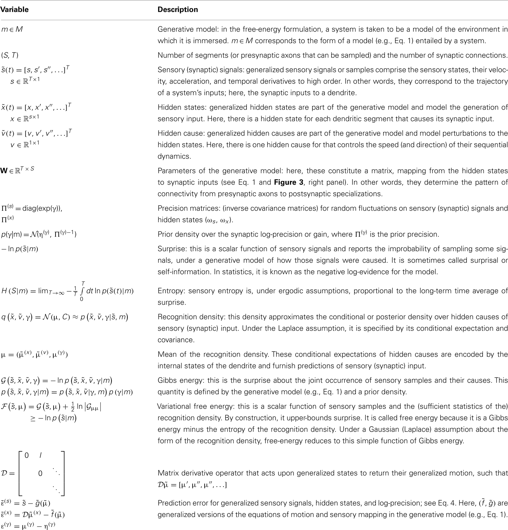
Table 1. Key quantities in the free-energy formulation of dendritic sampling and reorganization.

Free energy rests on a generative model of the sensory input a system is likely to encounter. This generative model is entailed by form and structure of the system (here a single neuron) and specifies its function in terms of the inputs it should sample. Free-energy minimization can be used to model systems that decode inputs and actively select those inputs that are expected under its model (Kiebel et al., 2008). Note that the Bayesian perspective confers attributes like expectations and prior beliefs on any system that conforms to the free-energy principle; irrespective of whether it is mindful (e.g., a brain) or not (e.g., a neuron). Using free-energy minimization, we have shown previously that many phenomena in perception, action, and learning can be explained qualitatively in terms of Bayesian inference (Friston et al., 2009; Kiebel et al., 2009b). Here, we apply the same idea to the dendrite of a single neuron. To do this, we have to answer the key question: what is a dendrite’s generative model? In other words, what synaptic input does a dendrite expect to see?

Differences in the morphology and connections among neurons suggest that different neurons implement different functions and consequently “expect” different sequences of synaptic inputs (Vetter et al., 2001; Torben-Nielsen and Stiefel, 2009). Recently (Branco et al., 2010) provided evidence for sequence-processing in pyramidal cells. By using in vitro two-photon laser microscopy, glutamate uncaging, and patch clamping, these authors showed that dendritic branches respond selectively to specific sequences of postsynaptic potentials (PSPs). Branco et al. (2010) found PSP sequences that move inward (toward the soma) generate higher responses than “outward” sequences (Figure 1C): Sequences were generated by activating spines along a dendritic branch with an interval of ca. 2 ms (Figures 1A,B). They assessed the sensitivity to different sequences using the potential generated at the soma by calcium dynamics within the dendritic branch. In addition, they found that the difference in responses to inward and outward sequences is velocity-dependent: in other words, there is an optimal sequence velocity that maximizes the difference between the responses to inward and outward simulation (see Figures 1C,D). These two findings point to intracellular mechanisms in the dendritic branches of pyramidal cells, whose function is to differentiate between specific sequences of presynaptic input (Destexhe, 2010). Branco et al. (2010) used multi-compartment modeling to explain their findings and proposed a simple and compelling account based on NMDA receptors and an impedance gradient along the dendrite. Here, we revisit the underlying cellular mechanisms from a functional perspective: namely, the imperative for self-organizing systems to minimize free energy.

FIGURE 1

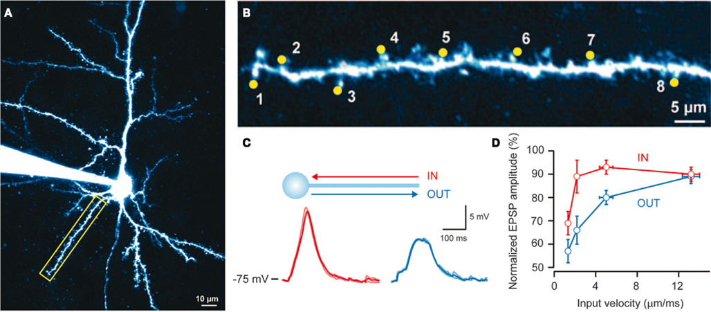
Figure 1. Findings reported by Branco et al. (2010): Single dendrites are sensitive to the direction and velocity of synaptic input patterns. (A) Layer 2/3 pyramidal cell filled with Alexa 594 dye; the yellow box indicates the selected dendrite. (B) Uncaging spots (yellow) along the selected dendrite. (C) Somatic responses to IN (red) and OUT (blue) directions at 2.3 mm/ms. (D) Relationship between peak voltage and input velocity (values normalized to the maximum response in the IN direction for each cell, n = 15). Error bars indicate SEM. Reproduced from Branco et al. (2010) with permission.

In brief, this paper is about trying to understand how dendrites self-organize to establish functionally specific synaptic connections, when immersed in their neuronal environment. Specifically, we try to account for how postsynaptic specializations (i.e., spines) on dendritic branches come to sample particular sequences of presynaptic inputs (conveyed by axons). Using variational free-energy minimization, we hope to show that the emergent process of eliminating and redeploying postsynaptic specializations in real neuronal systems (Katz and Shatz, 1996; Lendvai et al., 2000) is formally identical to the model selection and optimization schemes used in statistics and machine learning. In what follows, we describe the theoretical ideas and substantiate them with neuronal simulations.

Free Energy and the Single Neuron

Our basic premise is that any self-organizing system will selectively sample its world to minimize the free energy of those samples. This (variational) free energy is an information theory quantity that is an upper bound on surprise or self-information. The average surprise is called entropy; see Table 1. This means that biological systems resist an increase in their entropy, and a natural tendency to disorder. Crucially, surprise is also the negative log-evidence that measures the “goodness” of a model in statistics. By applying exactly the same principle a single dendrite, we will show that it can explain the optimization of synaptic connections and the emergence of functional selectivity, in terms of neuronal responses to presynaptic inputs. This synaptic selection is based upon synaptic gain control, which is itself prescribed by free-energy minimization: When a synapse’s gain falls below a threshold it is eliminated, leading to a pruning of redundant synapses and a selective sampling of presynaptic inputs that conforms to the internal architecture of a dendrite (Katz and Shatz, 1996; Lendvai et al., 2000). We suggest that this optimization scheme provides an interesting perspective on self-organization at the (microscopic) cellular scale. By regarding a single neuron, or indeed a single dendrite, as a biological system that minimizes surprise or free energy, we can, in principle, explain its behavior over multiple time-scales that span fast electrochemical dynamics, through intermediate fluctuations in synaptic efficacy, to slow changes in the formation, and regression of synaptic connections.

This paper comprises three sections. In the first, we describe the underlying theory and derive the self-organizing dynamics of a Bayes-optimal dendrite. The second section presents simulations, in which we demonstrate the reorganization of connections under free-energy minimization and record the changes in free energy over the different connectivity configurations that emerge. We also examine the functional selectivity of the model’s responses, after optimal reconfiguration of its connections, to show the sequential or directional selectivity observed empirically. In the third section, we interpret our findings and comment in more detail on the dendritic infrastructures and intracellular dynamics implied by the theoretical treatment. We conclude with a discussion of the implications of this model for dendritic processing and some predictions that could be tested empirically.

Materials and Methods

In this section, we present a theoretical treatment of dendritic anatomy and dynamics. Following previous modeling initiatives, we consider a dendrite as a spatially ordered sequence of segments (see, e.g., Dayan and Abbott, 2005, p. 217ff). Each segment expresses a number of synapses (postsynaptic specializations) that receive action potentials from presynaptic axons. Each synapse is connected to a specific presynaptic axon (or terminal) and registers the arrival of an action potential with a PSP. Our aim is to explain the following: If a dendrite can disambiguate between inward and outward sequences (Branco et al., 2010), how does the dendrite organize its synaptic connections to attain this directional selectivity? In this section, we will derive a model that reorganizes its synaptic connections in response to synaptic input sequences using just the free-energy principle.

We start with the assumption that the dendrite is a Bayes-optimal observer of its presynaptic milieu. This means that we regard the dendrite as a model of its inputs and associate its physical attributes (e.g., intracellular ion concentrations and postsynaptic gains) with the parameters of that model. In what follows, we describe this model, its optimization and consider emergent behavior, such as directional selectivity.

To illustrate the approach, we modeled a dendrite with five segments, each of which expresses four synapses: see Figure 2. This means the dendrite has to deploy T = 20 synapses to sample five distinct presynaptic inputs in a way that minimizes its free energy or surprise. The internal dynamics of the dendrite are assumed to provide predictions for a particular sequence of synchronous inputs at each dendritic segment. In other words, each connection within a segment “expects” to see the same input, where the order of inputs over segments is specified by a sequence of intracellular predictions: see Figure 3.

FIGURE 2

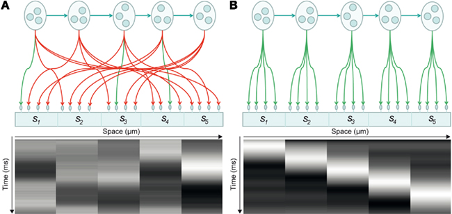
Figure 2. Synaptic connectivity of a dendritic branch and induced intracellular dynamics. (A) Synaptic connectivity of a branch and its associated spatiotemporal voltage depolarization before synaptic reorganization. In this model, pools of presynaptic neurons fire at specific times, thereby establishing a hidden sequence of action potentials. The dendritic branch consists of a series of segments, where each segment contains a number of synapses (here: five segments with four synapses each). Each of the 20 synapses connects to a specific presynaptic axon. When the presynaptic neurons emit their firing sequence, the synaptic connections determine the depolarization dynamics observed in each segment (bottom). Connections in green indicate that a synapse samples the appropriate presynaptic axon, so that the dendritic branch sees a sequence. Connections in red indicate synaptic sampling that does not detect a sequence. (B) After synaptic reconfiguration: All synapses support the sampling of a presynaptic firing sequence.

FIGURE 3

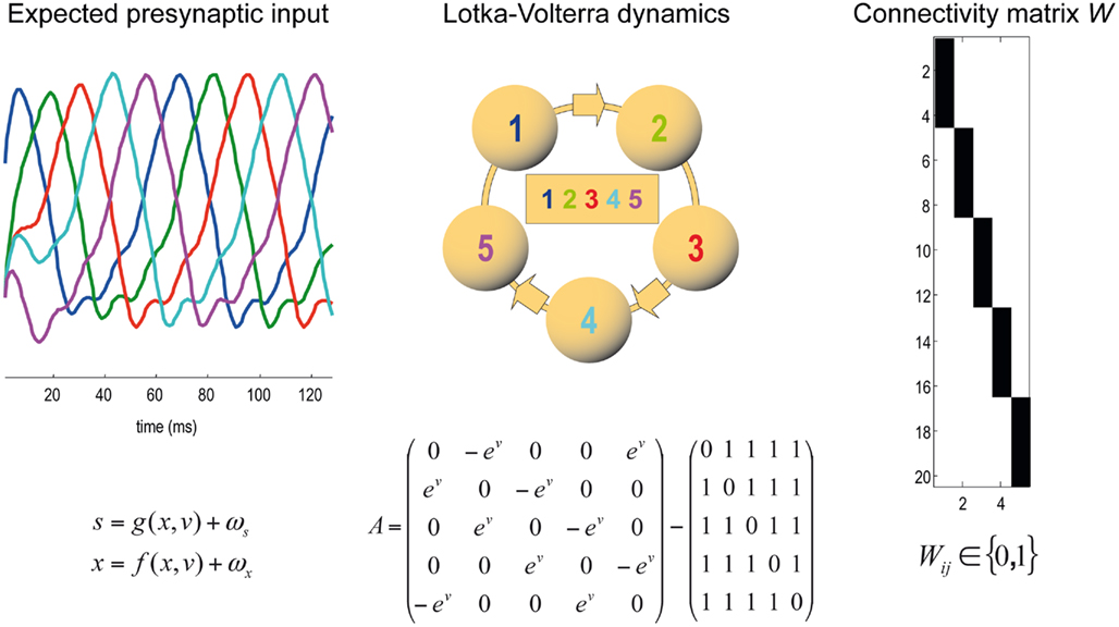
Figure 3. Generative model of dendritic branch dynamics. (Left) This shows the hidden states generating presynaptic input to each of five segments. These Lotka–Volterra (winnerless competition) dynamics are generated by Eq. 1in the main text. The inhibitory connectivity matrix A depends on the state v which determines the speed of the sequence. (Middle) The Lotka–Volterra dynamics are induced by the specific inhibitory connections among the five segments. In matrix A, we use the exponential of v to render the speed positive; this could be encoded by something like calcium ion concentration. (Right) The synaptic connectivity matrix W determines which presynaptic axons a specific synapses is connected to. An element W_ij in black indicates that there is a connection from presynaptic axon j to synapse i. Each synapse is connected to exactly one presynaptic axon; i.e., each row of matrix W must contain a single one and zeros elsewhere.

To minimize free energy and specify the Bayes-optimal update equations for changes in dendritic variables, we require a generative model of sequential inputs over segments. To do this, we use a model based on Lotka–Volterra dynamics that generates a sequence, starting at the tip of the dendrite and moving toward the distal end. In other words, the dendrite models its synaptic input S(t) = [S₁,…,S_T]^T as being caused by a saltatory sequence of changes in (hidden) states x(t) = [x₁,…,x_s]^T representing the presynaptic activity to which each segment is exposed. The speed at which the sequence is expressed is controlled by a hidden variable v(t) according to the following equations

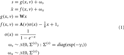
These equations model winnerless competition among the hidden states to produce sequential dynamics (called a stable heteroclinic channel; Rabinovich et al., 2006). Here, ω_s(t) ∈ ℝ^T and ω_x(t) ∈ ℝ^S correspond to random fluctuations on synaptic input and the hidden states respectively. These fluctuations have covariances (Σ^(s),Σ^(x)) or precisions (Π^(s),Π^(x)) (inverse covariances), where the precision of the i-th synaptic input is determined by its log-precision or gain: γ_i. Log-precisions are a convenient way to express variances because they simplify the update equations presented below.

The mapping from hidden states (presynaptic axons) to synaptic input is parameterized by a connectivity matrix W ∈ ℝ^T×S with elements W_ij ∈ ℝ{0, 1} that determine whether there is a synaptic connection between the j-th presynaptic axon and the i-th segment (Figure 3). It is this pattern of connections that determines the form of the model. The matrix A ∈ ℝ^{S × S} determines the sequential dynamics. For example, to generate a sequence for S = 4 segments, one would use:

In Eq. 2, the first matrix models exhibition and inhibition between neighboring segments and determines the sequence. We use the exponential of the hidden cause to ensure the speed e^v is positive. The second matrix encodes non-specific inhibition among segments.

Given this model of how synaptic inputs are generated, we can now associate the internal states of the dendrite with the model’s parameters or variables. In other words, we assume that the intracellular dynamics of the dendrite are trying to predict the input that it receives, based on the generative model in Eq. 1: see Figure 2B and Figure 3 (left panel). This means that we can cast dendritic changes as minimizing the free-energy associated with any given synaptic inputs. This provides Bayes-optimal update equations (i.e., non-linear differential equations) for each internal state. These equations describe how the internal states of a dendrite change when receiving input over time. A related application using winnerless competition in the context of sequence recognition can be found in Kiebel et al. (2009b). In the following, we will briefly describe the resulting update equations. Details of their derivation and implementation can be found in Friston et al. (2008). The key quantities involved in this scheme are described in Table 1.

Free-Energy Minimization

Minimizing the free-energy based on the generative model (Eq. 1) involves changing the internal variables of the dendrite so that they minimize free energy. Free energy is a function of the internal variables because they constitute Bayes-optimal predictions of the hidden states and synaptic input. In the present context, there are four sets of variables that can change 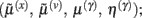these correspond to conditional expectations or predictions about hidden states and causes; predictions about synaptic log-precision or gain and predictions about existence of a synaptic input per se (see Table 1). As we will see below, optimizing these variables with respect to free energy is necessarily mediated at three distinct time-scales pertaining to (i) fast intracellular dynamics (e.g., depolarization and consequent changes in intracellular concentrations such as calcium): (ii) synaptic dynamics that change the efficacy or precision of synaptic connections and (iii) an intermittent selection and regeneration of postsynaptic specializations. Crucially, all three minimize free energy and can be expressed as a series of differential equations or update rules, as follows:

We now consider each of these updates in turn.

Fast Intracellular Dynamics (Eq. 3a)

Equation 3a represents the fastest time-scale and describes the predictions of hidden states associated with each dendritic segment and the hidden cause controlling the speed of the synaptic sequence. Later, we will associate these with depolarization and intracellular concentrations within the dendrite. The dynamics of this internal states correspond to a generalized gradient descent on free energy: ℱ, such that when free energy is minimized they become Bayes-optimal estimates of the hidden variables. This is the basis of Variational Bayes or ensemble learning and is used widely in statistics to fit or invert generative models, see Hinton and van Camp (1993), Friston (2008), Friston et al. (2008) for details. For those readers with a time-series background, Eq. 3a has the form of a generalized Kalman–Bucy filter and is indeed called Generalized Filtering (Friston et al., 2010). The reason it is generalized is that it operates on generalized states 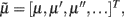where 𝒟 is a matrix derivative operator, such that . See Table 1 and Friston et al. (2010).

It can be seen that the solution to Eq. 3a [when the motion of the prediction is equal to the predicted motion ] minimizes free energy, because the change in free energy with respect to the generalized states is zero. At this point, the internal states minimize free energy or maximize Bayesian model evidence and become Bayes-optimal estimates of the hidden variables.

Gaussian assumptions about the random fluctuations in the generative model (Eq. 1) allow us to write down the form of the free energy and therefore predict the exact behavior of the dendrite. Omitting constants, the free energy according to Eq. 1is:

In these expressions, a subscript denotes differentiation. The expression for 𝒢 may appear complicated but the first three terms are simply the sum of squares of precision-weighted prediction errors. The last three equalities are prediction errors for the sensory states, hidden states, and log-precisions. The synaptic precisions; 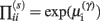depend on the optimized log-precisions or gains, where (η^(γ), Π^(γ)) are the prior expectation and precision on these log-precisions. In other words, the dendrite embodies the prior belief that γ ∼ 𝒩(η^(γ), Σ^(γ)).

Given Eq. 4, we can now specify the dynamics of its internal states according to Eq. 3a:

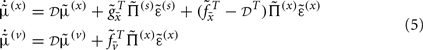
These equations describe the segment-specific dynamics and dendrite-wide dynamics that we associate with local depolarization, within each segment and intracellular (e.g., calcium ion concentrations) throughout the dendrite (see Discussion). The precision 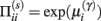can be regarded as the gain of a synaptic connection, because it modulates the effect of presynaptic input on internal states. This leads to the next level of optimization; namely, changes in synaptic gain or plasticity.

Synaptic Dynamics (Eq. 3b)

Equation 3b prescribes the dynamics of the log-precision parameter that we associate with synaptic efficacy or gain. Mathematically, one can see that the solution to Eq. 3b minimizes free energy, when both the change in efficacy and its motion are zero. This motion can be thought of as a synaptic tag at each connection that accumulates the prediction error on inputs. Under the model in Eq. 1, Eq. 3b becomes

This has a simple and plausible interpretation: the log-precision or gain has a tendency to increase but is counterbalanced by the precision-weighted sum of the squared error (e.g., potential difference) due to the inputs. When the noise is higher than predicted, the level of the synaptic tag will fall and synaptic efficacy will follow. The final two terms mediate a decay of the synaptic tag that depends on its prior expectation , see Eq. 4, where π is the (large) precision on prior beliefs that connections change slowly, see Friston et al. (2010). In the simulations, we actually update the efficacy by solving Eq. 6after it has been exposed to a short periods of inputs (128 time-bins). Finally, we turn to the last level of optimization, in which the form of the model (deployment of connections) is updated.

Synaptic Selection (Eq. 3c)

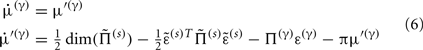
Equation 3c can be regarded as a form of Bayesian model selection, when the dendrite reconfigures its model in structural terms; that is, by redeploying synaptic connections through changing the matrix W. This is implemented using the free energy or log-evidence for competing models. For each connection, two models are considered: a model m₀ with a synapse that has a low prior log-precision and a model m₁ in which the connection has a high prior If the evidence for the model with a high prior (gain) is greater, then the synapse is retained. Intuitively, this procedure makes sense as model m₁ with high prior will be better than model m₀, if the internal states of the dendrite predicted the input (the dendrite sampled what it expected). Otherwise, if synaptic input is unpredictable (and model m₀ is better than m₁) the synapse is removed (regresses) and is redeployed randomly to sample another input. The corresponding odds ratio or Bayes factor for this model comparison is

Where corresponds to the all the presynaptic input seen between model updates. The details of this equality are not important here and can be found in Friston and Penny (2011). The key thing is that it is a function of the conditional density of the log-precision of the i-th connection The ensuing relative probabilities of models with and without a high-precision connection have the simple (sigmoid) form shown in Figure 4. The threshold appears at unity because it is half-way between the high (four) and low (minus two) prior expectations we allow the neuron to consider. In the present context, this means that a connection is retained when

FIGURE 4

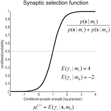
Figure 4. Synaptic selection function. This sigmoidal function measures the relative probability of two models with and without a high-precision synapse. The i-th synaptic connection is retained when ; i.e., there is more evidence that the synapse has high precision. If the synaptic connection is removed and a new, randomly chosen, presynaptic target is chosen. See also Eq. 7.

In summary, after the conditional log-precisions are optimized they are used to determine whether the synapse should be retained or replaced. This decision is formally identical to a model selection procedure and can be regarded as a greedy search on models m ⊃ W with different patterns of connections. In practice, we update the model after every four bursts (128 time points) of input.

Simulations and Results

Synaptic inputs were generated using the Lotka–Volterra system in Figure 3 and presented to the dendrite using simulated noise with a log-precision of two. Each simulated 128 time-bin time-series was presented over (64 × 4) repeated trials. The internal states of the dendrite evolved according to Eq. 3a and provide (Bayes-optimal) conditional expectations about the hidden states and cause of sampled inputs. We started with an initially random deployment of connections and changed them every four trials (after which the conditional estimates of log-precision had converged, see Eq. 3b). As described above, connections were only retained if the conditional log-precision was greater than one (see Figure 4). Otherwise, it was replaced at random with a connection to the same or another input. This slow model optimization or reorganization (Eq. 3c) was repeated over 64 cycles.

Figure 5 shows the results of the ensuing optimization of the connections, based upon free-energy minimization, at the three temporal scales (Eq 3). Since the optimization scheme converged after 30 iterations we only show the first 32 iterations. The middle panel shows that the negative free-energy increased as a function of pruning over cycles of reorganization. Note that this is a stochastic search, because the relocation of each connection was chosen at random. However, it is greedy because connections are retained if they provide a better model at that point in the search. Over time, the dendrite comes to sample presynaptic inputs in exactly the way that it expects to sample them. This means that each segment samples the same presynaptic axons (Figure 2B) and all five segments sample presynaptic inputs in a particular temporal sequence (a sequence prescribed by intracellular dynamics that rest on the generative model in Eq. 1). As the pattern of connections is optimized, the conditional log-precisions (or the gain) of the synaptic connections increases; as shown in the left panel of Figure 5. Usually, but not inevitably, once a synapse has found its place, in relation to others, it retains a relatively high log-precision, and is immune from further regression. Note that the fourth segment (synapses 13–16) converged quickly on a particular axon. After this, other segments start to stabilize, as confident predictions about their inputs enable the dendrite to implicitly discriminate between a good synapse (that samples what is expected) and a bad synapse (that does not). The sequence grows slowly until all 20 synapses have found a pattern that samples the five inputs in the order anticipated. This simulation is typical of the many that we have run. Note further, there is no unique pattern of connections; the sequence could “start” at any segment because (in this example) there was no prior constraint in the generative model that the first input would be sampled at any particular segment. Examples of synaptic connections are shown in the right panel of Figure 5 as “connectivity matrices” in the lower row for the 1st, 10th, 20th, and 32nd cycles. We see here a progressive organization from an initially random deployment to an ordered and coherent sequence that is internally consistent with the generative model.

FIGURE 5

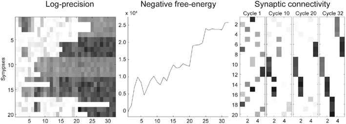
Figure 5. Reconfiguration of the synaptic connections for a dendritic branch with five segments and four synapses per segment. After 32 iterations, the scheme converged on the optimal solution. (Left panel): Correct (black) versus incorrect (white) synaptic gains (precisions) learned over iterations. (Middle panel): Temporal evolution of the objective function, the negative free energy. In most iterations, the free-energy decreases but there are sporadic setbacks: e.g., after the sixth iteration. This is due to the stochastic search, i.e., the random sampling of presynaptic axons. (Right panel): Snapshots of the connectivity matrix W (see Materials and Methods) after iterations 1, 10, 20, and 32.

Figure 6 shows the conditional predictions of synaptic input and hidden states before (upper row) and after (lower row) the synaptic pattern has been established. The right panels show the location of the connections in terms of expected log-precisions. The left panels show the predictions (solid lines) and prediction errors (red dotted lines) of synaptic inputs. Note that when the dendrite can predict its inputs (lower left) the prediction error (input noise) has a log-precision of about two (which is what we used when simulating the inputs). The predictions are based upon the conditional expectations of hidden states describing the Lotka–Volterra dynamics shown in the middle panels. Here, the solid lines correspond to the conditional expectations. After optimization, the predicted hidden states become quickly entrained by the input to show the stable sequential orbit or dynamics prescribed by the dendrite’s generative model. This orbit or attractor has a single control parameter v (Eqs 1 and 2) that the dendrite is also predicting and implicitly estimating (see below). Notice that this synchronous entrainment never emerges before reconfiguration (upper panels) and the sequence of expected hidden states is not the sequence expected a priori; deviations from this sequence are necessary to explain the seemingly unpredictable input. Note that there is still a winnerless competition and sequential itinerancy to the conditional (internal) dynamics, because there are strong priors on its form. However, the expected sequence has not been realized at this stage of synaptic reconfiguration.

FIGURE 6

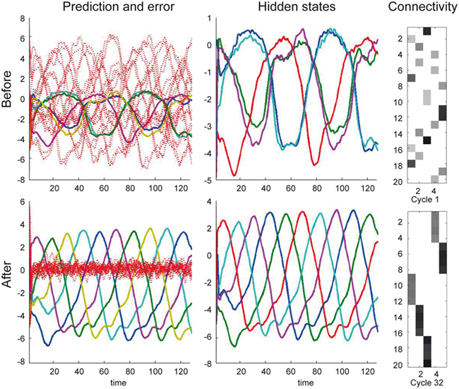
Figure 6. Intracellular dynamics for the simulation reported in Figure 5. (Top) Before synaptic reconfiguration, the intracellular dynamics do not follow the expected sequence, because the dendrite samples the presynaptic neurons in a random fashion. The left panel show the predictions (solid lines) and prediction errors (red dotted lines) of presynaptic inputs. The solid lines in the left and middle panels show the predictions (of x) that can be considered a fusion of the expected Lotka–Volterra dynamics and the sensory input. The right panel indicates the synaptic configuration (as expected log-precisions). (Bottom) Same representation as top panels but after synaptic reconfiguration is complete. The dendrite samples the presynaptic neurons such (right panel) that the expected Lotka–Volterra dynamics are supported by the input. Note that the prediction error (left panel) has a log-precision of about two (which is what we used when simulating the inputs).

It is worth noting that although relatively simple, this greedy search has solved a quite remarkable problem: It has identified a viable arrangement of connections in a handful of iterations, from an enormous number 5²⁰ of potential configurations. Once the pattern of connection weights has converged the dendrite has effectively acquired selectivity for the particular spatiotemporal pattern of inputs it originally expected. This is demonstrated in the next section.

Functional Specialization

In the simulations above, the prior on the synaptic noise had a low log-precision (minus two). The log-precision of the hidden states and cause was assumed to be 16; i.e., the precision of the hidden states was very high relative to synaptic precision. After the synaptic reorganization converged, we reduced the log-precision on the hidden states and causes to eight, to test the ability of the branch to correctly infer its inputs, even when less confident about its internal dynamics. In this context, the hidden cause reports the presence of a sequence. This is because when the hidden cause takes small values, the implicit speed of flow through the sequence becomes very small and, effectively, the sequence disappears.

Figure 7 illustrates the selectivity of postsynaptic responses to particular sequences of presynaptic inputs, using the hidden cause as a summary of postsynaptic responses. Each row of this figure corresponds to a different trial of 128 time-bins, in which we presented presynaptic inputs with different sequences. Each sequence was created by integrating a Lotka–Volterra system using a Gaussian bump function for the cause v(t), that peaked at v = 1 at time-bin 64 and adding noise in the usual way. The top row of Figure 7 shows the sequence the dendrite expects, as can be seen by the progressive temporal shift in presynaptic input over the 20 neurons (organized into five successive segments; upper left). The corresponding postsynaptic response, modeled in terms of the conditional expectation of the hidden cause, is shown on the upper right. This shows a sustained firing throughout the sequence. In contrast, if we present the identical presynaptic inputs but in a different sequence, this sustained response collapses to 0.5 (the default). This can be seen in the lower two rows for two arbitrary examples. The thin blue lines correspond to the conditional expectation of the hidden cause that controls the velocity of orbits through the stable heteroclinic channel. The gray areas correspond to 90% confidence intervals (tubes). The thick blue lines correspond to null firing and provide a reference. While the middle row contains no evidence of the expected sequence, the lower row contains two occurrences of the sequence between time point 40–60 and time point 80 (bottom left). These chance occurrences are promptly indicated by the postsynaptic response (bottom right). These graded responses between the maximum response (top right) and the minimum response (middle right) replicate another finding of Branco et al. (2010), who reported similar graded responses to random sequences.

FIGURE 7

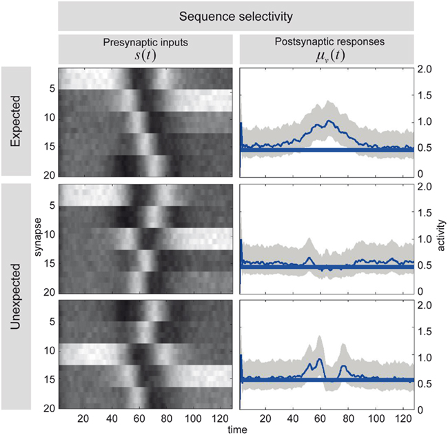
Figure 7. Sequence selectivity of dendritic response. Left column: Three waves of presynaptic inputs and their associated postsynaptic responses after successful reconfiguration (see Figure 6). Top: Inward sequence, where the wave progresses as expected by the branch, from the tip of the dendrite toward the soma. Middle and Bottom: Random sequences, with no specific order. Right column: The postsynaptic responses of the model to presynaptic input causing the three different depolarization waves. The post-response is modeled as the time-varying propagation rate exp(μ^(v)) (see Eq. 1). Top: For the inward sequence, the branch infers a rate of 1 during the presence of the sequence. The random sequences let the branch infer a rate of the default of 0.5 (no inward sequence present) 1 with brief excursions beyond the value of 0.5 when parts of the sequence were sampled (e.g., lower right plot around time points 40 to 60 and 80).

Velocity-Dependent Responses

Branco et al. (2010) were able to demonstrate a velocity-dependent selectivity in relation to inward and outward sequences of presynaptic activation (see Figure 1D). We attempted to reproduce their results using the above simulations by changing the velocity of the input sequence and presenting it in the preferred and reverse order: Presynaptic inputs were presented over 64/v time-bins for each of four velocities, v ∈ {1, 2, 4, 8}. We generated two presynaptic input sequences at each velocity, one with an inward and the other with an outward direction. Figure 8 shows the maximum response as a function of velocity for inward (red) and outward (blue) directions using the same format as Figure 1D (Branco et al., 2010). As with the empirical results, velocity-dependent responses are observed up to a certain ceiling. This ceiling (about v = 4 in these simulations) arises because the generative model cannot predict fast or high-velocity sequences, because of a (shrinkage) prior on the hidden cause. This means the hidden states are poor estimates of the true values and the hidden cause is underestimated as a consequence. However, within the range imposed by prior expectations, the response scales linearly with the true hidden cause (velocity). However, we were unable to reproduce the increase in the normalized response to the outward sequence as a function of velocity. It is an open question at what level this mismatch arises; e.g., at the level of the generative model presented above, which would call for a further adaptation of the model, or in terms of measuring its responses (note we report absolute as opposed to normalized responses).

FIGURE 8

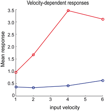
Figure 8. Velocity-dependent responses of the dendrite for the inward (red) and outward (blue) sequence. We modeled the response by the mean over the inferred time-dependent propagation rate (see right column of Figure 7) at four different speeds of the input sequence.

Discussion

We have described a scheme for synaptic regression and sampling that is consistent with the selectivity of dendritic responses of pyramidal cells to spatiotemporal input sequences (Branco et al., 2010); and is consistent with the principle of free-energy minimization (Friston et al., 2006). The scheme explains how a dendrite optimizes synaptic re-organization in response to presynaptic input to minimize its free energy and therefore produce Bayes-optimal responses. From a neurobiological perspective, the mechanism implied by the model is simple; intracellular states of a dendrite are viewed as predicting their presynaptic inputs. Postsynaptic specializations, with imprecise predictions (over a period of time) are retracted and a new dendritic spine is elaborated elsewhere. Over time, the dendrite comes to sample what it expects to sample and this self-limiting process of synaptic reorganization converges on an optimum pattern of synaptic contacts. At this point, postsynaptic responses become selective for the expected sequence of inputs. In the model, synaptic reorganization is described as model optimization at a slow time-scale (Eq. 7), which is based on free-energy minimization schemes at two faster time-scales (Eqs 5 and 6). Using simulations, we showed that this scheme leads to self-organized synaptic reorganization of a simulated dendrite and replicated two key experimental findings reported by Branco et al. (2010); directional selectivity and velocity-dependent responses.

Free-Energy Minimization and Intracellular Dynamics

The functional form of Eq. 5has an interesting and straightforward interpretation in terms of transmembrane voltage differences and conductances. The first equality of Eq. 5can be associated with the dynamics of transmembrane voltage in each segment. This suggests that the prediction errors in Eq. 4play the role of potential differences that drive changes in voltage according to Kirchhoff’s law (where the accumulation of charge is proportional to current). In other words, each term in Eq. 5corresponds to a current that is the product of a conductance and potential difference (prediction error). For example, in the second term, where, the synaptic input corresponds to local depolarization, while the generalized prediction of this depolarization, plays the role of a dynamic reference or reversal potential. The associated conductance depends upon the presence of a synaptic connection and the synaptic precision (gain). The conductance of the third term is more complicated and can be thought of in terms of active membrane dynamics of the sort seen in Hodgkin Huxley formulations of gating variables (e.g., Cessac and Samuelides, 2007). In short, our formal (Bayes-optimal) model of dendritic dynamics can be regarded as a mixture of currents due to active conductances that are entrained by synaptic currents. This is important because it means that the present model is consistent with standard models of active dendritic function; see Gulledge et al. (2005) for a review. Interestingly, we did not make any such assumption in the generative model (Eq. 1) but these active dendritic dynamics emerged as a functional feature of self-organization from free-energy minimization. An exciting prospect for future research is that one can ask how the generative model could be refined to replicate other experimental findings, such as spike timing dependent plasticity (STDP).

Although slightly more speculative, the kinetics of the hidden cause may correspond to slow dynamics, such as the calcium ion concentration. Although the associations with membrane voltage and calcium dynamics are hypothetical at this stage, we note they can be tested by using the dynamics described by Eq. 5as qualitative or even quantitative predictions of empirical dendritic responses (cf, dynamic causal modeling; Kiebel et al., 2009a).

Furthermore, to identify generative models from empirical observations, one can use the concept of generalized convolution kernels, which describe the mapping between dendritic input and output. The fact that neurons are selective for temporal sequences necessarily requires the kernels to have a long support and to be non-linear (a linear kernel would just average over time and not care about temporal order). Critically, one can derive these kernels analytically from the differential equations used in the present simulations (Eq. 5). It is possible to evaluate these kernels empirically by looking at their input–output characteristics (e.g., Pienkowski et al., 2009). This means, in principle, it is possible to infer the implicit generative models used by neurons and dendrites, given empirical estimates of their generalized (Volterra) kernels and use these models to test concrete predictions of what output should be observed given some defined input, e.g., provided by glutamate uncaging.

Dynamical Constraints

In our scheme, the intracellular dynamics of a dendrite encode the implicit expectation that input is sampled in a particular sequence. This is enforced by prescribing the form of intracellular dynamics (where the parameters governing these dynamics are fixed): the only variables that can change are estimates of the hidden states and the time-varying rate constant (Eq. 1). The only parameters that are optimized (Eq. 3b) are the connections to presynaptic inputs encoded by matrix W. This means that a dendrite can only stop re-organizing its synaptic connections when the postsynaptic effect of synaptic inputs are consistent with (predicted by) its intracellular dynamics. Intuitively, this behavior may be interpreted by an observer as if the dendrite is actively looking for a sequence in its input. This view is conceptually important because it suggests that single neurons cannot decode arbitrary synaptic input but implicitly expect specific spatiotemporal input patterns. This scheme may be considered slightly counter-intuitive: In the textbook view, the assumption is that neuronal networks should be decoders of arbitrary spatiotemporal input, thereby mimicking the generalization abilities of the brain (Hertz et al., 1991). In contrast, in the present scheme, a dendrite of a pyramidal cell is “cherry-picking” just those inputs that happen to form particular sequences. Input selectivity of this kind is not necessarily a surprise to neurophysiologists, because this hypothesis has been entertained for some time (Destexhe, 2010). It is reasonable to expect that neurons, whatever their apparent function, generally expect specific spatiotemporal patterns of synaptic input; where the morphology of a neuron (the dendritic infrastructure and ion channel distributions) place strong constraints on its function (Torben-Nielsen and Stiefel, 2009). The advantage of this selectivity may be that constraints simplify structural reconfiguration and learning because there are fewer free parameters to optimize (and fewer local minima to confound learning). In this paper, we provide some evidence that anatomic–dynamical constraints enable synaptic reorganization by self-organization of intracellular and synaptic dynamics.

Active Inference

In the model, the dendritic branch is optimizing its internal representation of presynaptic inputs at a fast time-scale (Eqs. 3a,b), while the dendrite’s implicit model of those inputs is itself optimized over longer time periods, using synaptic regression (Eq. 3c). Crucially, because model-optimization changes the way that presynaptic signals are sampled, this corresponds to a form of “active inference” or optimal sampling of the local environment. Conceptually, this sampling is based on model selection, which contrasts with the use of gradient descent schemes we have used in previous work (Friston et al., 2009). The model selection scheme used here is stochastic and necessarily slow due to the sampling of synapses that do not support a sequence. However, due to its stochastic nature, the scheme is more robust to local minima and may provide a useful metaphor for how real neuronal architectures are selected; cf, neuronal Darwinism (Edelman, 1987).

Robustness, Scalability, and Convergence Behavior

In the present paper, we did not evaluate the proposed scheme with respect to robustness to noise or artifacts, its scalability or its convergence behavior. Our aim was to provide proof of principle that free-energy minimization is a sufficient explanation for recent empirical observations about dendritic behavior. However, the present model was robust to noise and showed good convergence behavior within 64 iterations. We did not explore scalability, due mainly to computational reasons: the current implementation of free-energy minimization [dynamic expectation maximization (DEM), see software note] is relatively fast on a modern desktop computer (∼10 min) for small numbers of segments (five) but becomes prohibitive (with runtimes of hours) for dendrite models with more than 10 segments. We are currently working on a more efficient implementation and will report a thorough evaluation of the proposed algorithm and extensions in future communications.

Related Modeling Work

There are several computational treatments that share key features with the present modeling approach: Gutig and Sompolinsky (2006) have described a classification of input spike trains based on the membrane potential function of a point neuron. Although both their model and inference technique differ from the present approach, they share the idea that intracellular dynamics can be used to decode spatiotemporal input structure. We extend this notion and show that Bayesian inference for non-linear dynamical systems enables decoding based on dynamical generative models (such as Lotka–Volterra dynamics). A different idea is shared with the work by Deneve (2008) who considers single spiking neurons as Bayesian decoders of their input, where decoding dynamics map to neuronal and synaptic dynamics. This is exactly the view we take here but we use non-linear dynamical systems to describe the multi-dimensional internal state of a dendrite, as opposed to a single state representation of “the internal activation level.” In other words, we share the view that neurons are Bayesian decoders of their input but assume that a single neuron (dendrite) can represent many more variables than a single state. This enables us to describe spatiotemporal Bayesian decoding at multiple time-scales.

Conceptually, there is a strong link with the work of Torben-Nielsen and Stiefel (2009) where the function of a neuron (detecting the order of two inputs) is specified first, followed by an optimization of the neuron’s morphology and ion channel distribution, in relation to that function. This is similar to the free-energy formulation, where a generative model specifies the function by describing what input is expected. The subsequent free-energy minimization optimizes the neuronal system to perform this function using neurobiologically plausible intracellular dynamics. As in Torben-Nielsen and Stiefel (2009), the goal is to map the resulting inversion dynamics to the intracellular dynamics of real neurons.

Free-Energy Minimization at Different Scales

We have exploited free-energy minimization over three temporal scales in the dendritic simulations (intracellular dynamics, synaptic dynamics, and synaptic regression) and have framed these as model inversion and optimization respectively. Free energy can be minimized consistently over spatial and temporal scales because the underlying imperative is to minimize the sum or integral of free energy over all parts of the system and over all times. Because the time-integral of energy is called action, we are basically appealing to the principle of least action (Friston et al., 2008). Action here is fundamental and, mathematically, is an upper bound on the entropy of presynaptic inputs. In short, by minimizing surprise (self-information) at fast temporal scales, systems can place upper bounds on their entropy and therefore resist a natural tendency to disorder; i.e., they resist the second law of thermodynamics.

In terms of network formulations of free-energy minimization; how does recognizing sequences of presynaptic inputs help at the neuronal network level? The answer to this question may rest on message-passing schemes in cortical hierarchies that can be understood in terms of free-energy (prediction error) minimization (Mumford, 1992; Rao and Ballard, 1999; Friston, 2005; Kiebel et al., 2008; Friston and Kiebel, 2009). A key aspect of these schemes is that they are based on prediction error units that report the generalized motion (local trajectory) of mismatches between bottom-up presynaptic inputs and top-down predictions (Friston et al., 2008). This necessarily entails a selective response, not to input patterns at any instant in time, but patterns over time. But how does a neuron learn what to respond to? In this paper, we have avoided this question and assumed that the neuron has a pre-ordained generative model (prior expectations) of its local presynaptic milieu. This model rests upon the form and parameters of internal dynamics; i.e., the form and parameters of Lotka–Volterra dynamics. Clearly, in the real brain, these parameters themselves have to be learned (optimized). Future research may show the utility of free-energy minimization at different spatial and temporal scales to relate learning at the single neuron and network level.

Software Note

The simulations described in this paper are available (in Matlab code) within the DEM Toolbox of the SPM Academic freeware (http://www.fil.ion.ucl.ac.uk/spm). To reproduce the figures in this paper, type “DEM_demo” at the Matlab prompt and select “Synaptic selection” from the user interface.

Conflict of Interest Statement

The authors declare that the research was conducted in the absence of any commercial or financial relationships that could be construed as a potential conflict of interest.

Acknowledgments

Karl J. Friston was funded by the Wellcome Trust. Stefan J. Kiebel was funded by the Max Planck Society. We thank Katharina von Kriegstein and Jean Daunizeau for helpful discussions.

References

Branco, T., Clark, B. A., and Hausser, M. (2010). Dendritic discrimination of temporal input sequences in cortical neurons. Science 329, 1671–1675.

Pubmed Abstract | Pubmed Full Text | CrossRef Full Text

Cessac, B., and Samuelides, M. (2007). From neuron to neural networks dynamics. Eur. Phys. J. Spec. Top. 142, 7–88.

Daunizeau, J., Friston, K. J., and Kiebel, S. J. (2009). Variational Bayesian identification and prediction of stochastic nonlinear dynamic causal models. Physica D 238, 2089–2118.

Pubmed Abstract | Pubmed Full Text | CrossRef Full Text

Dayan, P., and Abbott, L. F. (2005). Theoretical Neuroscience. Cambridge, MA: The MIT Press.

Deneve, S. (2008). Bayesian spiking neurons I: inference. Neural Comput. 20, 91–117.

Pubmed Abstract | Pubmed Full Text | CrossRef Full Text

Destexhe, A. (2010). Dendrites do it in sequences. Science 329, 1611–1612.

Pubmed Abstract | Pubmed Full Text | CrossRef Full Text

Destexhe, A., and Huguenard, J. R. (2000). Nonlinear thermodynamic models of voltage-dependent currents. J. Comput. Neurosci. 9, 259–270.

Pubmed Abstract | Pubmed Full Text

Edelman, G. M. (1987). The Theory of Neuronal Group Selection. New York: Basic Books.

Feynman, R. P. (1972). Statistical Mechanics; a Set of Lectures. Reading, MA: W. A. Benjamin.

Friston, K. (2005). A theory of cortical responses. Philos. Trans. R. Soc. Lond. B Biol. Sci. 360, 815–836.

Pubmed Abstract | Pubmed Full Text

Friston, K. (2008). Hierarchical models in the brain. PLoS Comput. Biol. 4, e1000211.

Pubmed Abstract | Pubmed Full Text | CrossRef Full Text

Friston, K. (2010). Is the free-energy principle neurocentric? Nat. Rev. Neurosci. 11, 607–608.

Friston, K., and Kiebel, S. (2009). Predictive coding under the free-energy principle. Philos. Trans. R. Soc. Lond. B Biol. Sci. 364, 1211–1221.

Pubmed Abstract | Pubmed Full Text

Friston, K., Kilner, J., and Harrison, L. (2006). A free energy principle for the brain. J. Physiol. Paris 100, 70–87.

Pubmed Abstract | Pubmed Full Text | CrossRef Full Text

Friston, K., and Penny, W. (2011). Post hoc Bayesian model selection. Neuroimage 56, 2089–2099.

Pubmed Abstract | Pubmed Full Text | CrossRef Full Text

Friston, K., Stephan, K., Li, B. J., and Daunizeau, J. (2010). Generalised filtering. Math. Probl. Eng. 2010, Article ID: 621670.

Friston, K. J. (2009). Modalities, modes, and models in functional neuroimaging. Science 326, 399–403.

Pubmed Abstract | Pubmed Full Text | CrossRef Full Text

Friston, K. J., Daunizeau, J., and Kiebel, S. J. (2009). Reinforcement learning or active inference? PLoS ONE 4, e6421.

Pubmed Abstract | Pubmed Full Text

Friston, K. J., and Dolan, R. J. (2010). Computational and dynamic models in neuroimaging. Neuroimage 52, 752–765.

Pubmed Abstract | Pubmed Full Text | CrossRef Full Text

Friston, K. J., Trujillo-Barreto, N., and Daunizeau, J. (2008). DEM: a variational treatment of dynamic systems. Neuroimage 41, 849–885.

Pubmed Abstract | Pubmed Full Text | CrossRef Full Text

Gulledge, A. T., Kampa, B. M., and Stuart, G. J. (2005). Synaptic integration in dendritic trees. J. Neurobiol. 64, 75–90.

Pubmed Abstract | Pubmed Full Text | CrossRef Full Text

Gutig, R., and Sompolinsky, H. (2006). The tempotron: a neuron that learns spike timing-based decisions. Nat. Neurosci. 9, 420–428.

Pubmed Abstract | Pubmed Full Text

Hertz, J., Krogh, A., and Palmer, R. G. (1991). Introduction to the Theory of Neural Computation. Redwood City, CA: Addison-Wesley Publishing Company.

Herz, A. V. M., Gollisch, T., Machens, C. K., and Jaeger, D. (2006). Modeling single-neuron dynamics and computations: a balance of detail and abstraction. Science 314, 80–85.

Pubmed Abstract | Pubmed Full Text | CrossRef Full Text

Hinton, G. E., and van Camp, D. (1993). “Keeping the neural networks simple by minimizing the description length of the weights,” in COLT ‘93 Proceedings of the Sixth Annual Conference on Computational Learning Theory, 5–13.

Katz, L. C., and Shatz, C. J. (1996). Synaptic activity and the construction of cortical circuits. Science 274, 1133–1138.

Pubmed Abstract | Pubmed Full Text | CrossRef Full Text

Kiebel, S. J., Daunizeau, J., and Friston, K. J. (2008). A hierarchy of time-scales and the brain. PLoS Comput. Biol. 4, e1000209.

Pubmed Abstract | Pubmed Full Text | CrossRef Full Text

Kiebel, S. J., Garrido, M. I., Moran, R., Chen, C. C., and Friston, K. J. (2009a). Dynamic causal modeling for EEG and MEG. Hum. Brain Mapp. 30, 1866–1876.

Kiebel, S. J., von Kriegstein, K., Daunizeau, J., and Friston, K. J. (2009b). Recognizing sequences of sequences. PLoS Comput. Biol. 5, e1000464.

CrossRef Full Text

Lendvai, B., Stern, E. A., Chen, B., and Svoboda, K. (2000). Experience-dependent plasticity of dendritic spines in the developing rat barrel cortex in vivo. Nature 404, 876–881.

Pubmed Abstract | Pubmed Full Text | CrossRef Full Text

London, M., and Hausser, M. (2005). Dendritic computation. Annu. Rev. Neurosci. 28, 503–532.

Pubmed Abstract | Pubmed Full Text

Mel, B. W. (2008). “Why have dendrites? A computational perspective,” in Dendrites, eds G. Stuart, N. Spruston, and M. Hausser (New York: Oxford University Press), 421–440.

Mumford, D. (1992). On the computational architecture of the neocortex.2. The role of corticocortical loops. Biol. Cybern. 66, 241–251.

Pubmed Abstract | Pubmed Full Text | CrossRef Full Text

Pienkowski, M., Shaw, G., and Eggermont, J. J. (2009). Wiener-Volterra characterization of neurons in primary auditory cortex using Poisson-distributed impulse train inputs. J. Neurophysiol. 101, 3031–3041.

Pubmed Abstract | Pubmed Full Text | CrossRef Full Text

Rabinovich, M. I., Varona, P., Selverston, A. I., and Abarbanel, H. D. I. (2006). Dynamical principles in neuroscience. Rev. Mod. Phys. 78, 1213–1265.

Rao, R. P., and Ballard, D. H. (1999). Predictive coding in the visual cortex: a functional interpretation of some extra-classical receptive-field effects. Nat. Neurosci. 2, 79–87.

Pubmed Abstract | Pubmed Full Text

Spruston, N. (2008). Pyramidal neurons: dendritic structure and synaptic integration. Nat. Rev. Neurosci. 9, 206–221.

Pubmed Abstract | Pubmed Full Text

Torben-Nielsen, B., and Stiefel, K. M. (2009). Systematic mapping between dendritic function and structure. Network 20, 69–105.

Pubmed Abstract | Pubmed Full Text | CrossRef Full Text

Vetter, P., Roth, A., and Hausser, M. (2001). Propagation of action potentials in dendrites depends on dendritic morphology. J. Neurophysiol. 85, 926–937.

Pubmed Abstract | Pubmed Full Text