Effective connectivity modeling for fMRI: six issues and possible solutions using linear dynamic systems

Introduction

One goal of cognitive neuroscience is to understand how cognitive level variables (e.g., behavioral responses and actions, mental states, disorders of cognition related to disease, etc.) can be mapped onto variables associated with the biology of the brain. Functional magnetic resonance imaging (fMRI) allows for non-invasive observations of signals indirectly related to local field potentials (LFP) and to a lesser extent integrated neural firing rates (Logothetis et al., 2001; Logothetis and Pfeuffer, 2004; Logothetis, 2008). The sampling rate of fMRI is typically around 0.5–1 Hz though higher rates are possible. Spatial resolution of fMRI is typically around 16 mm³. These signals can be acquired approximately simultaneously throughout the brain. Much of the focus in fMRI image analysis over the last 20 years has been on the localization of aspects of cognitive processes. Through analysis of regional responses via mass-univariate statistics, specific functions have been “localized” to or identified with specific brain regions and structures. Recently, more interest has been focused on how local computations in specialized areas are integrated with computations in other task related regions. Analysis of the task related integration of multiple regions is referred to a connectivity analysis (Horwitz et al., 1999; Friston, 1994; Horwitz, 2003).

Several methods have been proposed to analyze task related integration operationally defined as inter-regional covariance or related statistical dependency such as correlation analysis, principle components regression, independent components regression, graphical models, and partial least squares (Moeller and Strother, 1991; Horwitz et al., 1992; McIntosh et al., 1994, 1996; Bullmore et al., 1996; McKeown et al., 1998; Andersen et al., 1999; Lohmann and Bohn, 2002; Smith et al., 2006; Sporns et al., 2007; Bullmore and Sporns, 2009). This type of analysis, often referred to as functional connectivity, typically ignores the temporal properties of the data and focuses instead on the identification of multiple spatially disparate regions that are inter-related via non-causal statistical dependencies. Functional connectivity is taken to indicate regions that respond to specific trials or instances of a task in a similar manner rather than simply regions which respond to generically to the task. The dependency of functional connectivity measures on this trial-to-trial and moment-to-moment variability with a given task is most obvious in trial correlation methods (c.f., Rissman et al., 2004) but within task variability forms the theoretical basis of all functional connectivity measures (Horwitz et al., 2005).

Also of interest are methods that attempt to identify directionality or causality in the interactions between regions. Directionality of integration can be defined in terms of temporal relations (i.e., causes precede consequences) and/or information flow (i.e., variation at one site typically coincides with variation a second cite though variation at the second does not always coincide with variation at the first). These directional connections are often referred to as “effective connectivity” (Friston, 1994). Because of computational limitations, effective connections are often calculated among a small number of regions of interest (ROIs) believed to be of primary importance for the task (though see Valdes-Sosa, 2004; Roebroeck et al., 2005; Valdes-Sosa et al., 2005; Abler et al., 2006; for whole brain approaches).

A number of methods have been proposed for effective connectivity analysis including structural equation modeling, multivariate autoregressive modeling, dynamic Bayesian models, bilinear dynamic systems, switching linear dynamic systems, and dynamic causal modeling (DCM; McIntosh and Gonzalez-Lima, 1992; Buchel and Friston, 1997; Friston et al., 2003; Harrison et al., 2003; Penny et al., 2005; Rajapakse and Zhou, 2007; Smith et al., 2010). Each method has its own specific set of assumptions and benefits and different methods are often framed to address slightly different questions. A full review of the various effective connectivity methods is beyond the scope of the current discussion. A descriptive review and evaluation of many methods has been presented elsewhere (e.g., Smith et al., 2011).

Despite wide-spread use of these effective connectivity methods, several theoretical, and practical issues remain unresolved. Here, six issues important to the development and application of effective connectivity models are identified and discussed in turn¹. The first issue concerns the use of deterministic versus stochastic models to identify effective connectivity. We argue that stochastic models capture the notion of connectivity better than deterministic models, we show that deterministic models provided little if any information independent of task related activation, and we demonstrate that the type of stochastic model matters. The second issue is concerned with the level of variability in connectivity parameter values in effective connectivity models. Most estimates of effective connectivity are constant within conditions or even scan runs in the case of resting state experiments. We show how a joint modeling approach can be used to estimate continuously varying connectivity parameters. We discuss limitations of the joint model approach and then consider a mixture of multiple models approach that addresses these limitations. The third issue concerns identifying the optimal number and location of regions to include in a connectivity model. We present the first objective approach to determining the number of regions to include in a effective connectivity model based on dynamic systems theory. We further show how augmented dynamic systems can be used to identify the location of additional regions missing from a connectivity model. The fourth issue addresses the problem of identifying the optimal voxel(s) in an a priori defined anatomic region to include in a connectivity model. Often researchers wish to include signals from anatomical regions based on a priori hypotheses concerning the connectivity network. However these hypotheses do not specify the specific location within a given anatomical area. We show how dynamic systems and sparse canonical correlations can be combined within a single model to identify “optimal” voxels from a region. The fifth issue concerns the interpretation of connectivity parameter values. We argue that identified connectivity parameter values can only be interpreted within the context of the other parameters. We introduce orthogonal impulse response functions, a common network analysis method in econometrics, to fMRI connectivity analysis to identify the effect of a change in one region upon the other regions of the network. The sixth issue concerns the effect of the slow hemodynamic response to brief neural events on the temporal accuracy of connectivity models. We argue for and briefly describe a simple statistical combination of simultaneous EEG and fMRI within the same dynamic system. Discussion of each issue is presented at a level intended to be of use to practitioners and consumers of connectivity models as well as developers. For didactic reasons, a general linear dynamic system for fMRI (LDSf; Penny et al., 2005; Smith et al., 2010) framework is presented to facilitate discussion of the issues in concrete terms. LDSf is a simple model making it easy to understand, and it is highly flexible making it easy to extend to deal with these issues. Possible remediation for each issue is presented in the LDSf framework. While the extensions of the LDSf system summarized here are useful advances, they are incomplete; open questions remain to be addressed by further research.

Linear Dynamic Systems for fMRI

The form of a discrete time, stochastic LDSf is presented in Eqs 1 through 3². The

intent of the LDSf model framework is to model the multiregional observed fMRI time series as the hemodynamic consequences of the same number of quasi-neural level variables (Penny et al., 2005; Smith et al., 2010). The quasi-neural level variables are themselves functions of the interactions between these variables. In Eq. 3, the n-dimensional vector y_t is the measurement or observation of the system at time t where t varies from 1 to T, the total number of observations. For ease of exposition and without loss of generality, the time index is set to the scanner time to repeat (TR). Each y_i variable is the known fMRI time series from a single region, often detrended or band-pass filtered, and standardized so each time series has zero mean and unit variance. Thus, y_it identifies the observation of the ith region at time t.

The n-dimensional quasi-neural level time series x_t in Eq. 1 is unobserved and must be estimated from the data. These hidden states are assumed to be conditionally Gaussian [i.e., P(x_t | y_1:t) ~ N(x_t, P_t)] and are linear functions of the previous hidden state x_t−1 with additive noise The state transition matrices describe the directed interactions among the hidden states and can be thought of as defining the effective connectivity among the regions. The matrices represent the effect of known exogenous inputs v_t on the quasi-neural variables. The superscript u_t indicates multiple matrices indexed by the variable u. If u does not vary (i.e., u_1:T = 1), the quasi-neural system in Eq. 1 is simply a linear ARX(1) model with Gaussian error. At the other extreme where u_t = t, all quasi-neural system matrices vary through time resulting in a highly non-linear, heteroscedastic system. In between these extremes (i.e., u ∈ {1:p}; p ≪ T), the quasi-neural system in Eq. 1 is a piece-wise linear approximation to a non-linear heteroscedastic system, often referred to in the literature as an intervention model (Hamilton, 1989; Lütkepohl, 2007). It can be assumed that the number of system matrices is equal to the number of experimental conditions with u_t thus being an indicator variable identifying the condition at time t; in this case the variable u_t is referred to as the cognitive regime (Smith et al., 2010).

In Eq. 2, the variable Z_t simply contains h errorless lagged copies of x from x_t−(h−1) to x_t. The observation, y_t, is an instantaneous linear function of Z_t and additive noise ζ_t ~ N(0, R) with R_ij = 0 for i ≠ j. The matrix Φ is an a priori known set of basis vectors that span the variability in the hemodynamic response function such as a canonical hemodynamic response and its derivatives with respect to time and dispersion (Penny et al., 2005). The matrix β contains regionally specific weights for these bases to generate a regionally unique hemodynamic impulse response function β_iΦ. The linear output β_iΦZ_it is thus equivalent to convolving each quasi-neural variable with its regional hemodynamic response. Importantly, each quasi-neural level variable is associated with one and only one output variable thus localizing the quasi-neural level time series. It is assumed that the observation and state errors are temporally white and uncorrelated; E[ε_t ε_t+τ] = E[ζ_t ζ_t+τ] = E[ε_t ζ_t] = 0. It is also possible to vary β with the cognitive regime if an experimenter believed her manipulations would directly alter the regional hemodynamic response. The observation error variance R can also be allowed to vary if noise such as movement related errors were believed to vary with experimental condition. These cases of varying observation equations are not considered further here.

Given the observations of the system y_1:τ and knowledge of the system matrices and sequence of cognitive regimes, one can infer the states of the dynamic system, x_t. Since the quasi-neural states are conditionally Gaussian, this can be achieved by identifying the mean and covariance that parameterize the normal distribution P(x_t|y_1:τ,u_1:τ). Identifying the mean and covariance of P(x_t|y_1:τ, u_1:τ) can be done efficiently using the Kalman filter for τ = t or using smoothing algorithms such as the Rausch Tung Striebel smother for τ > t (Shumway and Stoffer, 1991; Murphy, 1998; Bar-Shalom et al., 2001; Haykin, 2002). Note that the Gaussian assumption on x_t is only within a regime, if p > 1 then the full x time series is a mixture of Gaussians. Time series with multiple outliers or other leptokurtic distributions can be easily accommodated by using a regime with having large values on the diagonal.

Of primary concern in identifying effective connectivity models is identifying the parameters of the system matrices, β, and R. Optimal parameter estimation is a complex topic and beyond the scope of the current discussion. Most methods rely on gradient assent on the LDSf complete data log likelihood function

where T_u is the number of observations in regime u³, x₀, and P₀ are the initial state mean and covariance and | | is the determinant. A simple yet effective means of identifying parameters that maximize this likelihood is the expectation maximization algorithm (EM; Dempster et al., 1977), In the EM algorithm, an initial guess at the parameter values is used and the likelihood of the data given the parameters calculated. This calculation involves running a Kalman filter to identify the innovations variance and an RTS type smoother to identify the optimal state space distributions given the data and set of parameters θ, P(x_t|y_1:T, u_1:T, θ; Shumway and Stoffer, 1991; Kim, 1994; Murphy, 1998). The zero point of the partial derivatives of the log likelihood function with respect to each of the parameters is calculated and used to update the estimates of each of the parameters (Ghahramani and Hinton, 1996). The process is continued until the change in the calculated log likelihood drops below a threshold. Other methods such as Quasi-Newton gradient ascent or Variational Bayes are also used (Ghahramani and Hinton, 1998; Beal and Ghahramani, 2001; Doucet and Andrieu, 2001; Oh et al., 2005; Lütkepohl, 2007). Comparisons of some of these methods for similar systems have been discussed elsewhere and will not be examined here (c.f., Makni et al., 2008; Ryali et al., 2011).

An important point often ignored is that these parameter identification methods are only guaranteed to identify local maxima in the likelihood function; different initial guesses can produce different parameter estimates. Stopping criteria for the gradient ascent can be easily fooled by areas in parameter space with near-flat surfaces in the likelihood function. It is beneficial to attempt the maximization multiple times with different starting conditions to better identify globally optimal parameters. Once identified, the model and its parameters can be used to identify the quasi-neural time series for multiple runs and multiple subjects performing the same task (Smith et al., 2010).

The theoretical limit on the number of parameters that can be identified for an LDSf model is Tp − 1 where T is the number of time points and p is the number of regions while the number of parameters to be identified scales as s(2p² + pv) + (h + 1)p where s is the number of regimes, v the number of inputs and h the leading dimension of the hemodynamic basis. Thus the minimum number of scans to identify a model is s(2p + v) + h + 1. The practical limit is certainly much lower. Assuming 400 time points in a run (TR = 1.5 for 10 min), no inputs, and a requirement of 10 times the minimum number of data points necessary, 18 regions can be reasonably included in a model with a single condition, 9 in a model with two conditions, 6 in a model with three and so on. However, multiple runs of the same task in the same subject can be easily combined to increase the observations and thus the number of regions in the model; doubling the number of runs roughly doubles the number of regions that can be modeled.

The LDSf model is quite similar form and intent to DCM (Friston et al., 2003). Both estimate the states of an unobserved quasi-neural signal from a small number of regions based on an explicit forward model of the hemodynamic response. The forward model of DCM is non-linear and biophysically based while the forward model of LDSf is linear and pragmatically based (see Friston et al., 2000; Riera et al., 2004; Valdes-Sosa et al., 2011). However, any non-linearity in the hemodynamic response is negligible for block designs or event related designs with inter-trial intervals greater than approximately 3 s. Thus the two forward models can be expected to yield nearly identical hemodynamic responses in these cases. The DCM state equations are formulated in continuous (i.e., using derivatives) rather than discrete (i.e., using differences) time as used in the LDSf model. However, a direct relation between the continuous time and discrete time transition matrices exists via the matrix exponential and matrix logarithm⁴. Furthermore, assuming the sampling rate is fixed and constant as is the case in fMRI, estimating a discrete time model and converting it to continuous time will produce an essentially equivalent model to estimating the continuous model directly (Ljung and Willis, 2010).

There are significant differences between LDSf and DCM. DCM was originally intended as a hypothesis driven method while LDSf can be used in a more exploratory manner (Smith et al., 2010; Stephan et al., 2010; Friston et al., 2011). Because the LDSf model is linear in both state and output space, identifying parameters of the LDSf model can be more efficient than in DCM and a larger number of regions can be included in the model. The most important difference however is that the LDSf model is stochastic while DCM is deterministic. We examine this difference as the first issue.

Issue One: Stochastic Versus Determinism

The first issue concerns the choice of deterministic or stochastic models for use in identifying connectivity. Essentially this is the question of which effective connectivity model to use in an analysis. While often answered based on popularity alone, the choice of deterministic versus stochastic model determines the sources within the fMRI signal that are assumed to reflect connectivity. Functional connectivity has typically been associated with inter-regional relations among data variability (Horwitz et al., 2005). In early PET studies, the variability was related to coherent changes across subjects (Moeller and Strother, 1991; Horwitz et al., 1992; Alexander and Moeller, 1994). If the observed signal values of a set of regions maintained a consistent relationship across subjects, they were identified as functionally connected. This notion of connectivity was also used in early effective connectivity studies (McIntosh and Gonzalez-Lima, 1992). In fMRI data, the variability is across time from trial-to-trial or moment-to-moment. Early effective connectivity methods applied to fMRI such as PPI and SEM considered the residual variability between regions after main effects of task were removed (Horwitz et al., 2005). This trial-to-trial and moment-to-moment variability in fMRI is known to reflect coherent signals relevant to human perception and performance (Wagner et al., 1998; Pessoa et al., 2002; Ress and Heeger, 2003; Pessoa and Padmala, 2005; Fox et al., 2006).

In deterministic models, such as the original DCM for fMRI, the interactions between the quasi-neural level variables are completely determined by the dynamic model. That is, given a starting point, x₀, the value of x_t for any t ≥ 0 would be completely known for any known set of inputs and regime vector. In the LDSf framework this is equivalent to setting and thus ε_t to 0 for all t. The system may still contain measurement error (i.e., ζ_t ≠ 0), but the time course of the quasi-neural variables are determined and known with complete certainty given x₀. Further observations of the system are not necessary; once x₀ is known and given the model, the fMRI data at later times are superfluous.

In contrast, in a stochastic model the quasi-neural states are not completely determined by their previous values. For example, consider a stochastic LDSf system with constant A and Q matrices. Given a known quasi-neural state defined by a known mean and covariance in n-dimensional space, x₀ and P₀, the value of x₁ is a hyper-ellipsoid probability density centered at Ax₀ with semi-axes scaled by Q via

The probability distribution of x_t flows through time according to the eigenvectors of A. Without new observations of the system, the magnitude of the variance will spread over time until eventually the true state is essentially unknown. Each observation y_t provides additional evidence regarding the location of x_t, decreasing the uncertainty of its value.

If all sources of the trial-to-trail variability were known, quantifiable and measured using a few variables and the sampling rate was sufficient such that each observation could be labeled accurately by some combination of these known variables, a deterministic system would be appropriate for capturing connectivity. If the sources are unknown, the deterministic system cannot capture the trial-to-trial variability and thus cannot fully capture connectivity. Figure 1 shows the neural level responses over time during two blocks identified by a deterministic DCM model of the attention to visual motion paradigm (Buchel and Friston, 1997) as estimated by SPM5 according to the online example instructions (http://www.fil.ion.ucl.ac.uk/spm/data/attention/).The neural signals of the deterministic DCM were identified by modifying the function spm_int.m (1044 2007-12-21 20:36:08Z) included in the SPM5 software package to return the values of the state variables over time as well as the estimated hemodynamics. Also shown in Figure 1 are the quasi-neural responses during the same two blocks as estimated by a stochastic LDSf model. As seen in the figure, directional connectivity in the deterministic model is reflected in variation in the slope of the response onset for the block. Response onset slope is sharpest in V1 and decreases in V5 and even further in SPC. The consequence of this connectivity model is that the neural response in V5 to attended visual motion takes 5 s to achieve its 50% level while the SPC remains less than 75% of its maximal response even after 9.2 s of the task. This slow, monotonically increasing neural response to visual stimulation seems at odds with data from in vivo recordings where onsets of LFPs would be effectively instantaneous at the 3.22-s sampling rate of the fMRI data (Buracas et al., 1998; Liu and Newsome, 2006). In contrast, the stochastic LDSf estimate shows an early response to attended visual motion in all regions and interactions between the regions are reflected in the covariance in moment-to-moment response levels within the block.

FIGURE 1

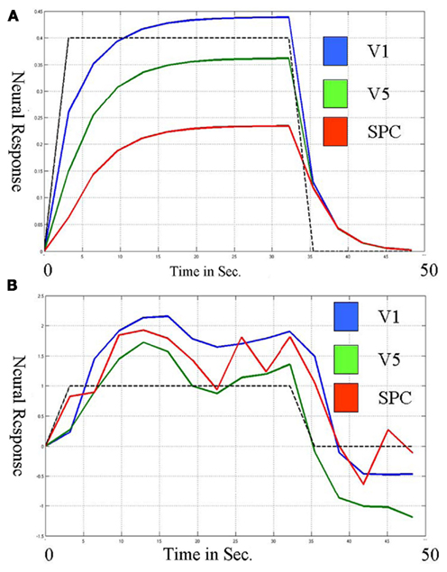
Figure 1. Neural responses over a single block (~30 s.) in three regions during the Attention to Visual Motion task as estimated via deterministic (A) and stochastic (B) models. (A) Connectivity in the deterministic (DCM) model is seen in the slope of the block onset. The region V1 (blue) increases first and most rapidly and V5 (green) increases with a similar slope. The region SPC (red) increases more slowly; its slope is less similar to V5 than V5 is to V1, thus the connectivity from V5 to SPC is less than that from V1 to V5. This slope magnitude and slope similarity is the nature of the deterministic connectivity. (B) In contrast, the three regions respond similarly in the onset of the block for the stochastic model. The connectivity is in the covariance within the block. V1 and V5 are more connected than V5 and SPC because their estimated responses are more correlated within the block.

The source of stochastic is also important. Ryali et al. (2011) propose a bilinear form of the LDSf model. The quasi-neural system dynamics of their model are

If Λ is an input matrix with columns Λ_i containing binary values identifying presence or absence of a experimental condition, the bilinear and multiple model forms can produce equivalent deterministic behavior by setting A^u = A + BΛ_i; that is, a separate A^u for each unique BΛ. However, the stochastic behavior of the two systems is not equivalent as Q, the covariance of the state noise, does not vary from condition to condition in the bilinear form. This is of critical importance as Q is used to derive measures of instantaneous (sub-sampling rate) connectivity.

It can be shown that under mild assumptions, models in the form of Eqs 1 and 6, which are in so called “reduced form,” can be transformed into an equivalent “structural form”

Here Ω is a diagonal matrix containing the variance of the innovation δ, accounts for instantaneous connectivity, and is a new autoregressive coefficient matrix. The conversion from one form to another is achieved via the relation

The number of unknown elements in that can be identified is restricted (Sims, 1980; Lütkepohl, 2006, 2007; Sims and Zha, 2006). Elements of can be identified by maximum likelihood methods as in Structural Equation Modeling, or more simply by factoring into a lower triangular matrix. The LDL factorization, which factors a Hermitian matrix A into a matrix L that is lower triangular with ones on the diagonal and a diagonal matrix D such that A = LDL′, has been frequently used to identify instantaneous connectivity in autoregressive models (Sims, 1986). The matrix L then contains the (acyclic) connectivity while D contains the residual, orthogonal, error variance. Thus by using a constant Q, the discrete time bilinear model of Ryali et al. (2011) assumes identical instantaneous connectivity between conditions.

Examining an LDSf model of the attention to visual motion data, bootstrap (Sims and Zha, 1999; Benkwitz et al., 2000) analysis shows none of the inter-regional connections in the A^u matrices is robustly different from 0. Thus there is no inter-regional AR(1) connectivity in this dataset. This is not particularly surprising given the 2.33-s sampling rate. However, bootstrap analysis on the instantaneous connections revealed significant changes in inter-regional connectivity between conditions (see Table 1). The bilinear form would miss these effects. To the extent that task dependent inter-regional interactions occurring faster than the Nyquist frequency exist in the data, the bilinear form will produce an erroneous result.

TABLE 1

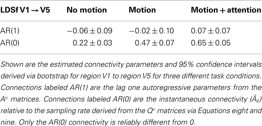
Table 1. LDSf identified connectivity between V1 and V5 in during the attention to visual motion task.

While the stochastic model is better reflective of the common notion of connectivity and does not produce the aberrant behavior of the deterministic model, it remains unclear if the stochastic model accurately reflects behavioral or neural level responses. The responses shown are still smooth but can have substantial ringing when the data are over-fit. The output equation used in the LDSf framework was originally proposed in the context of single voxel deconvolution (Penny et al., 2005). Penny et al. (2005) observed considerable within block variability similar to that shown in Figure 1B. However, as they note, these quasi-neural time series are only estimates, and other different time series can potentially be identified for the same data. This is essentially a result of the shape of the hemodynamic impulse response function. As can easily be seen in its Fourier transform, the canonical impulse response used in the SPM software package (Wellcome Trust Centre for Neuroimaging UCL, London) essentially passes zero information at high frequencies. Deconvolution can be performed as division in frequency space where the spectrum of the convolved signal is divided frequency-by-frequency by the spectrum of the filter to produce the spectrum of the unfiltered signal. However, in the high frequency portion of the signal, above approximately 0.2 Hz, this naive deconvolution in frequency space is dividing by almost zero, resulting in enormous estimated power. Care must be taken to avoid extreme high frequency shifts. In LDSf, this can be achieved by keeping the diagonal values of R at a high enough level to avoid ringing. Further tests with known within block response level changes are needed to better determine if identified quasi-neural level changes reflect these known task changes within blocks or trials. Fast and slow variations should be examined to see if there are limits to the time scales of quasi-neural level response changes that can be observed with these methods.

Issue Two: Parameter Variation

The second issue concerns the extent of the variability of connectivity parameters in effective connectivity models. Essentially this is the question of how and when connections between regions are allowed to change. Despite the complexity of identifying and validating effective connectivity models, the types of models examined to date are actually quite simple. Inter-regional interactions (connections) are typically held constant within task conditions and are repeated without variation over multiple instances of the same task condition (though see Ge et al., 2009; Havlicek et al., 2010, 2011). Connectivity parameter variation is used only to induce changes in response patterns between conditions. Within condition variability in the regional response is ignored in deterministic models and treated as the result of unmodeled interactions and/or input in stochastic models.

An additional or alternative means to model trial-to-trial within condition variability is by allowing the inter-regional connectivity to vary within as well as between task conditions. In the extreme, the cognitive regime can vary at each time point by setting u = [1:T]. This allows for a different connectivity pattern at each time point. With different parameters for each time point, the linear equations of the LDSf model can be used to approximate data from highly non-linear systems. However, the parameters of the model can no longer be identified using gradient assent methods as the number of parameters far exceeds the number of observations. Methods do exist to identify the model parameters provided additional assumptions are made regarding how the connectivity parameters change over time. One well studied method is to treat the elements of the system matrix A (i.e., the connectivity parameters) as time series generated by another dynamic system (Cox, 1964; Nelson and Stear, 1967; Ljung, 1979; Nelson, 2000; Wan et al., 2000; Wan and van der Merwe, 2001; Ge et al., 2009). The connectivity parameters can vary smoothly over time via a random walk with a fixed variance, Σ, as in Eq. 10 where θ_t are the connectivity parameters at time t.

Slow parameter dynamics can be achieved by using relatively small values on the diagonal of Σ and/or including additional autoregressive terms into the random walk. With a known dynamic model for the parameters, filtering methods can be used to estimate P(θ|y) in a similar manner as P(x|y). A so called “joint model” representation is formed by including the unknown parameters θ as part of the state space. For example, if only the system matrix A is allowed to vary at each time point, the joint state space update equation would be

This joint model is no longer linear and requires the use of non-linear filters for identification.

The possible utility of the joint model for temporally varying state transition parameters is briefly presented here using the unscented Kalman filter (UKF; Julier et al., 1995) for state estimation (see Havlicek et al., 2011 for a similar method). The UKF is a non-linear filter designed to efficiently estimate the propagation of a Gaussian distribution through any arbitrary non-linear function with third order accuracy and propagation of an arbitrary non-Gaussian distribution with at least second order accuracy (Julier et al., 1995; Wan and van der Merwe, 2001). This compares favorably to other methods such as the extended Kalman Filter and similar filters based solely on first order Taylor series approximations. The UKF operates by approximating an n-dimensional Gaussian with 2*n + 1 points selected deterministically to optimally reflect the distribution. These points are then propagated through the non-linear function and recombined for a new estimate. Thus the UKF can be considered a special case of the more flexible (and computationally intensive) particle filter although with deterministic particle sampling. Since the true non-linearity is used in the UKF no derivative information is needed.

Five hundred observations of a three region LDSf model were simulated using known parameters and an assumed TR of 1 s. Orthogonal white noise was added to both the state and observations with SD of 0.2 and 0.1 respectively. The observations of the model were generated by convolving the state space with a canonical hemodynamic response. Of the nine inter-regional connectivity parameters, the autoregressive self-connections were set to constant values, four off diagonal connections were set to zero, and the remaining two parameters, from region 1 to region 2 and from region 1 to region 3, were allowed to vary [0:1] according to 1/175 Hz cosine and sine waves respectively. A joint model of the resulting time series was identified using a combination of UKF and the EM algorithm. Variance of the random walk was set to 0.1. The UKF was used to estimate a joint state consisting of the quasi-neural state and all nine connectivity parameters. Estimates from a “forward” UKF and “backward” (i.e., temporally reversed) UKF were combined to create smoothed estimates [i.e., P(x_t,θ_t|y_1:T); Wan and van der Merwe, 2001]. These estimates were used to update the remaining model parameters via EM. The smoothed estimates are shown in Figure 2. Values of the static connections remain fairly close to their true values though there is substantial variation of the parameter values through time. The connection from region 1 to region 2 appears quite accurate and the connection from region 1 to region 3 captures at least some of its correct shape.

FIGURE 2

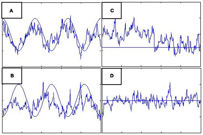
Figure 2. Actual connectivity parameter values from simulation (smooth lines) versus LDSf parameter estimates using the joint model (jagged lines). True parameter values in (A,B) vary according to sine waves while true parameter values in (C,D) are constant.

Further research is needed to determine the applicability of the joint model for temporally varying connectivity parameters in real fMRI data. The ability of the joint model to track changes in connectivity without knowledge of any task parameters suggests this method may be particularly useful for resting state and similar constant task paradigms. Unfortunately, the joint modeling method is ill-suited for most active task paradigms. The variance parameters of the random walk in Σ govern how quickly the parameters can change over time. To account for abrupt, non-smooth changes in connectivity that likely occur at the boundary between task conditions these parameters must be set to large values. The large variance allows the connectivity parameters to make large “jumps” to their new values. However, if Σ is held constant, large values would also increase the assumed variance of the parameters within each task condition. The within condition connections would then be free to attempt to non-smoothly vary in response to any noise in the data. This can be seen in Figure 2 where the joint model identified parameter variability as the source of variance in the states when the variance was due to noise. Thus the applicability of joint modeling to fMRI remains an open question.

What is needed is a model framework that can produce smooth, slow changes while allowing abrupt changes when necessary. Recently, an LDSf type model was introduced that can deal with both of these types of changes. The switching linear dynamic system for fMRI (SLDSf) can produce infinite variability over time in connectivity parameter values including instantaneous connectivity by probabilistically mixing a small number of static model regimes (Smith et al., 2010; see Murphy, 1998 for more detail on switching linear dynamic systems in a general context). Smith et al. (2010) discuss varying the cognitive regime over a small set, u ∈ {1:s} where s ≪ T. The probable value of u_t can be estimated by assuming Markovian dynamics for u given by a transformation probability matrix Π as

with P(u₀) = π. The probabilities of each regime can then be used for a “soft-filtering” update on the expected value (mean) of the state variable at time t as

where W_tj = P(u_t = j | y_1:t), x_jt is the expected value of x_t assuming regime j, and K_jt and ξ_jt respectively are the Kalman gain and innovation associated with regime j at time t. Similar formulas can be given for “soft-smoothing.” In Smith et al. (2010), a three regime model was identified for a single subject performing a finger alternation task with three conditions: tap left, tap right, and rest. This three regime model was then used to estimate the quasi-neural state x_t and probability of each regime P(u_t = j) at each time point for the same data, a second run of the same subject performing the same task with a different task ordering, and two runs from a second subject performing the same task. Results are shown in Figure 3. Probabilities for each regime are plotted along with a grayscale code of the correct task. The time course of the combined connectivity weights are also shown for several connections. Fast weight changes are seen at block onsets when regime probabilities change dramatically while slow weight variability is seen within blocks where regime probabilities are more stable.

FIGURE 3

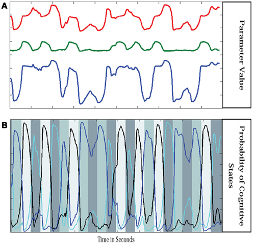
Figure 3. Parameter values in switching linear dynamic system. Shown are the parameter values for three regions (A) and the probability of each cognitive regime (B). Parameters are mixtures of the stationary models from each regime weighted by the probability of being in each regime. The connectivity parameter values are similar but not identical for repetitions of the same condition and the parameters vary within a block of the same condition as well. However the main source of variance in the parameters is the change from condition to condition.

A mixture of only a few different regimes may be insufficient to adequately model a given set of tasks. In the SLDSf model, the number of regimes does not need to be equal to the number of known tasks. Additional regimes can be identified for different portions of blocks, different stages of the scanning run, as well as “noise” regimes with identity state transitions and large, approximately uniform variance to account for outliers (c.f., Murphy, 1998). An alternative to increasing the number of regimes may be to combine a Viterbi SLDSf (i.e., only the most probable regime is active) and joint UKFs. Smooth parameter variations within a regime can be modeled by the joint filter with a small random walk variance while large or abrupt parameter transitions can be modeled as regime changes. This method is a candidate for future study in the context of fMRI. It is also possible to simultaneously learn the boundaries or regimes as well as the regime parameters with only an assumption on the number of regimes. Modeling a priori unknown regime boundaries may be particularly useful for resting state studies or studies with patient populations.

Switching linear dynamic system for fMRI models are not without problems. Of particular concern for fMRI is the standard approximation used in SLDS smoothing due to Kim (1994). While smoothing, the true smoothed regime probabilities P(u_t = j | u_t+1 = k, y_1:T) are typically approximated as P(u_t = j | u_t+1 = k, y_1:t) to avoid computational complexity. The approximation is considered relatively accurate provided the future observations (y_t+1:y_T) do not provide much additional information about u_t beyond that contained in u_t+1 (Kim, 1994; Murphy, 1998). Obviously this is not the case for fMRI where the hemodynamic response causes a substantial delay in the observable consequences of neural changes. This can produce overly smooth regime probabilities that rely heavily on Π and less on the observed data. Other methods exist that do not rely on this approximation (Barber, 2006) and are likely needed for better application to fMRI, particularly for fast regime switches as seen in event related designs.

Issue Three: Region Number and Location

The third issue concerns the number and location of regions to-be-included in effective connectivity models. This is essentially the question of how many regions one should include in a model and where are they? If the model is too limited, the danger of spurious influence is increased and if the model has too many degrees of freedom, the danger of over-fitting, and poor generalization is increased (Roebroeck et al., 2011). Hypotheses derived from existing theories concerning the location of the to-be-included regions are often based on anatomical structures or Brodmann areas. As such they are spatially imprecise relative to the resolution of fMRI data. Structurally defined regions may contain thousands of voxels with heterogeneous responses. Dimension reduction of the structure via Principle Components Analysis may result in signals that represent the variance within the structure, but not necessarily the variance in the structure associated with other areas. Using t statistics from univariate task analyses to select voxels identifies voxels with minimal variance beyond that explainable by the task. As discussed in Issue One, this minimizes the within task variance assumed to underlie connectivity.

Smith et al. (in review) present a principled approach for dealing with these two issues. Singular spectrum analysis (SSA; Broomhead and King, 1986; Vautard and Ghil, 1989; Ghil et al., 2002) is used to estimate the number of variables to include in the network. The augmented LDSf method of Smith et al. (2010) is then extended to identify multiple regions to-be-included in dynamic connectivity models starting from a single seed region.

The problem of the number of nodes needed in a connectivity network can be formalized as the number of variables required to generate observed data. Fortunately the problem of the number of variables operating in a non-linear dynamic system has been studied in other fields (Schouten et al., 1994; Abarbanel, 1995; Patel and Haykin, 2001). It has been proven (Whitney, 1936; Mañé, 1981; Takens, 1981) that the number of interacting variables in a dynamic system can be reliably estimated from observations of any smooth function of any number of the variables in the system. Thus it is theoretically possible to identify the number of variables active in the dynamic system operationally defined as “a brain performing a task” by observing data from one variable (voxel) involved in the network. While Takens’ theorem holds for noiseless systems, for noisy systems other researchers have developed a related concept of Statistical Dimension, defined as the number of variables in a dynamic system that can be reliably identified above noise from a specific data set (Vautard and Ghil, 1989; Sardanyés and Solé, 2007). The magnitude of the signal relative to the noise imposes limitations on how well the number of variables can be identified. Thus the Statistical Dimension of the data series is a function not only of the dimension of the true underlying dynamic system, but also the quality of the observations of that system (e.g., for fMRI data, the quality of the observations will be related to the field strength, TR, subject movement, etc.). The number of regions to include in a dynamic connectivity model can be determined by identifying the Statistical Dimension of the system.

Singular spectrum analysis is a method for estimating the Statistical Dimension of any arbitrary non-linear system corrupted by noise (Packard et al., 1980; Broomhead and King, 1986; Vautard and Ghil, 1989; Cheng and Tong, 1992; Kimoto and Ghil, 1993; Read, 1993; Plaut and Vautard, 1994; Allen and Smith, 1996; Ghil et al., 2002 and references therein). Full discussion of SSA is beyond the scope of this article. Briefly, SSA involves the Eigen-decomposition of a delay matrix, Ψ, created by concatenating m-length data vectors, Y_t, from sliding windowed views of the full data y_1:T

The covariance of Ψ will have p eigenvalues from the signal and m−p eigenvalues for the noise. Assuming white noise with uniform spectral power, the m−p eigenvalues associated with the noise will all be approximately equal and the p signal eigenvalues will be larger than this noise “floor” (Broomhead and King, 1986; Abarbanel et al., 1993). Pairs of equal eigenvalues occur when one variable is oscillating while unique eigenvalues occur for non-oscillating variables.

To demonstrate the utility of SSA, Smith et al. (in review) apply the method to the well known Lorenz attractor system (Lorenz, 1963)

A scalar observation signal was created from the product of the three x variables numerically integrated using Fourth Order Runge Kutta (further details are in Smith et al., in review). The first 20 eigenvalues obtained by SSA for varying window (m) sizes are plotted in Figure 4. Clearly, the first six eigenvalues form into three pairs of equivalent eigenvalues and eigenvalues past number six are all roughly equivalent to each other forming the noise floor. Frequency analysis of the eigenvectors confirms that each pair consists of a single frequency pattern differing from each other only by phase. Thus, each pair defines a single oscillating variable and the correct number of variables, three, was identified for the Lorenz Attractor system. Smith et al. (in review) also applied the SSA method to determine the dimension of the left motor cortex in a finger alternation task.

FIGURE 4

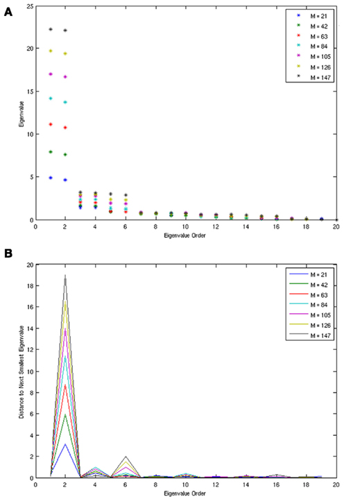
Figure 4. The eigenvalues (A) and eigenvalue spacing (B) identified by SSA for the Lorenz system at varying window sizes. Eigenvalues are correctly identified in three pairs, each pair representing a single variable from the system. The three pairs clearly rise above the zero floor.

When the locations of the regions participating in a network are not all known a priori, LDSf can be extended to identify missing regions (Smith et al., 2010). To maintain localization of the quasi-neural state space, the dimension of this state space is set equal to the dimension of the hemodynamic observations and a one-to-one mapping from neural states to hemodynamic observations is enforced. Smith et al. (2010) showed how additional regional signals could be identified by increasing the dimension of the neural state beyond the dimension of the hemodynamic observations while maintaining the one-to-one mapping. The additional neural dimension cannot directly influence the hemodynamic observations, but can interact with the other localized quasi-neural variables via the transition matrices The time series of the additional quasi-neural variable along with the localized variable(s) can be estimated using Kalman filtering and RTS smoothing as above (see Smith et al., 2010). Once identified, the time series of the additional quasi-neural variable at each time point can be convolved with a canonical hemodynamic response function, and used to predict each voxel in the brain via linear regression. The best fitting voxel is then the most likely candidate to be added to the model.

Issue Four: Voxel Selection

The fourth issue concerns the location of the optimal voxel from an a priori selected anatomical region to include in an effective connectivity model. This is essentially the question of which voxel should I use? While building up models from data alone is useful, often specific anatomic structures are of interest to researchers who wish to test hypotheses regarding the interactions between that structure and others. However, these hypotheses are often vague relative to the spatial frequency of the data as even relatively small structures such as entorhinal cortex can still contain several hundred voxels that do not all have a uniform response. Larger structures, such as fusiform gyrus, contain multiple distinct functional regions, the total number, and boundaries of which may not be known a priori. Further problems may be caused by the possibility that the optimal locus of inter-regional interaction within a structure may change from one task condition to the next. Selecting the exact voxel or combination of voxels to use in connectivity analyses has been a subject of continuing research (Goncalves and Hall, 2003; Spiridon et al., 2005; Friston et al., 2006; Saxe et al., 2006; Deleus and Van Hulle, 2009; Cole et al., 2010; Van Dijk et al., 2010; Marrelec and Fransson, 2011).

The most common method is to use univariate t statistics from task regression analysis to identify the most task related voxels within an anatomical region of interest and then use that voxel or small region of interest centered on that voxel as a node of the network. This method has obvious surface validity and reflects the secondary position of connectivity analysis in most functional imaging studies. That is, researchers often first seek to answer the functional localization question of which voxels responded most robustly to a task and only then attempt to address the functional integration question. However, t statistics represent ratios of known to unknown variability. The known variability is often impoverished consisting of little more than a uniform response to each instance of the task. The unknown variability thus contains both meaningful trial-to-trial variability as well as noise from measurement error or other sources. Selecting a voxel via t-ratios may lead to identification of voxels that are minimally affected by precisely the trial-to-trial variability that we wish to analyze as connectivity. What is necessary then is to identify task related voxels that have maximal variability associated with connectivity but minimal additional noise; suggesting that localization and integration should be computed concurrently. In continuous task or resting state experiments, t statistics are not available. Here again, while anatomical regions may be known (e.g., posterior cingulate and superior parietal cortex) the exact locations maximally connected between these regions are not known.

The most straightforward solution is to alter the output equation to allow multiple voxels to be associated with a single neural time course

where Y_i and Y_j represent different anatomical region 2. The vector Y_it is n by 1 in dimension where n is the number of voxels in the anatomical region. The vector ω_i is an n by 1 vector of voxel weights. If Φ is a single basis vector (e.g., canonical hemodynamic response only) ω_i can be identified by setting β_i to one and solving for 1/ω_i via maximum likelihood

where P_i is the maximum likelihood estimate of Note the similarity between this update and the regression solution. A separate ω can be identified for each regime (i.e., ω^u) to allow for task related differences in voxel weights.

To be identifiable, this regression based method requires that the hemodynamic response in each voxel of the anatomical region be a multiple of the single basis Φ. Substantial deviation between the true hemodynamic responses in the region and canonical basis may produce erroneous results. A more significant problem with the above method is the regression formulation. It can be shown that the Kalman filter solution to the multi-voxel LDSf model above will minimize the sum over t for the following cost function

where X_t|yi is the maximum likelihood estimate of P(x_t | y_1:i). The first term in Eq. 22 is a squared error in hemodynamic space. Thus it is clear that the above regression method will attempt to minimize the error for all voxels in the anatomical region. This will have the effect of steering ω⁻¹ toward the first eigenvector of the anatomical region. To the extent that the anatomical region is uniform, the summation over the error in all voxels is not a problem, but this negates any benefit of the above method over reducing the region to a single vector via Principle Components Analysis.

An alternative method is to replace the first squared error term of the cost function in Eq. 22 with a new one based on canonical correlations as in Eq. 23.

The solution to Eq. 23 is ω and β that maximize the correlation between Y and Z. Unlike Principle Components (eigenvector analysis) or Partial Least Squares, Canonical Correlations does not include a penalty for the variance accounted for within a region. All that is required is that the correlation between the weighted Y and Z is maximized. The number of voxels from the region participating can be minimized and spurious correlation avoided by using a sparse canonical correlation which maximizes the correlation while setting the majority of the elements of ω to zero (Parkhomenko et al., 2009).

The utility of the combination of sparse canonical correlations and LDSf is demonstrated via a simple simulation. Five hundred observations of an LDSf model with five quasi-neural variables were simulated as above using known parameters and an assumed TR of 1 s. Quasi-neural variables one through three were mutually interconnected as were variables four and five thus forming two distinct subnetworks. No connections existed between the two subnetworks however a common input vector was used for variables three through five (see Figure 5). Orthogonal white noise was included in both the state and observations with SD of 0.2 and 0.1 respectively. Observations for the first two regions of the model were generated by convolving their state space with a canonical hemodynamic response. One hundred “voxels” of a third anatomical region were simulated by mixing the time series of variables three through five according to weights as shown in Figure 5. All weights were non-zero. These mixed time series were convolved with a canonical hemodynamic response. One hundred data sets were generated from this model with different noise series. Three region LDSf models using the modified sparse canonical correlation cost function were then identified for each data set. Results of a typical run are shown in Figure 6 as is a histogram of the correlations between the estimated quasi-neural time series of the multi-voxel region and the third variable which constituted the “true” network variable. A clear preference for voxels from near the maximum of the correct weight distribution is evident. Thus the modified LDSf method was capable of selecting a voxel participating in the true generative network from a larger non-uniform anatomical region.

FIGURE 5

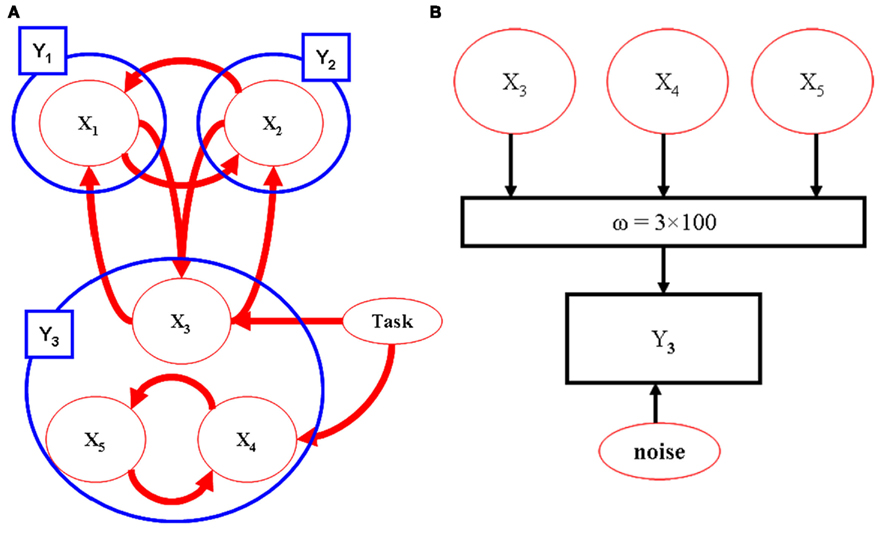
Figure 5. Model used for CCA-LDSf simulations. Model connectivity is shown in (A). The model contains three anatomical regions (blue circles). Regions 1 and 2 contain a single signal each while region three contains three signals (red circles). The signals form two distinct task related networks [1,2,3] and [3,4,5]. (B) For anatomical region 3, 100 voxels were created by mixing signals 3, 4, and 5 by known weights that varied by voxel. The weights were always non-zero and positive.

FIGURE 6

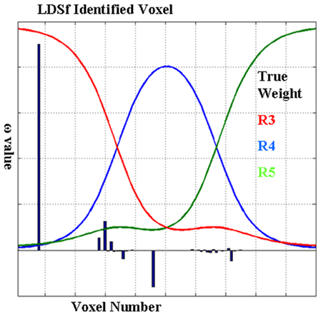
Figure 6. Results from the CCA-LDSf model. CCA-LDSf was used to identify a small number of “best” voxels from the 100 voxels in region 3 that interacted with regions 1 and 2 (see Figure 5). Signal three contains the optimal signal. Voxels with high weights on signal three (red weights) should be selected while voxels with low weights on signal three should be avoided. Values of weights for each voxel as estimated by the CCA-LDSf model are shown in bars. A voxel with near maximal true weight on signal 3 was chosen as the optimal voxel by the CCA-LDSf.

While the modified sparse canonical correlation LDSf is promising, it is not without potential pitfalls. The sparseness constraint results in a dramatic increase in the number of local minima of the likelihood function that is maximized to identify the model parameters. Poor choice of starting values or early settling on a sparse set of voxels may produce dramatically different results. Research toward determining better parameter identification methods as well as exploration of additional constraints such as non-negativity will be necessary before the method can be more generally applied. In addition, the simulations used here have a limited relation to real fMRI data. The results should be considered a proof of concept only. Further testing with real fMRI data is needed.

Issue Five: Parameter Interpretation

The fifth issue concerns the interpretation of the parameters identified in an effective connectivity model. This is essentially the question of now that I have a model, how do I know what it means? The typical focus of effective connectivity studies is the value of the connectivity parameters (i.e., the elements of the matrices or similarly the A and B matrices in DCM). Questions such as “is the connection parameter non-zero?” or “is the connection parameter different between these conditions?” are common. In LDSf, multiple means can be used to assess the statistical robustness of parameters and parameter differences. Variational Bayesian methods of parameter identification naturally provide uncertainty parameters for the identified connections (Makni et al., 2008; Ryali et al., 2011). These variances are then easily used to assess parameter robustness. If parameters are identified using Quasi-Newton methods, the estimated information matrix (inverse Hessian) can be used to approximate parameter variances and thus t tests (Lütkepohl, 2007). The information matrix can also be calculated independently using matrix derivative methods (Smith et al., 2010). The information matrix based methods are known to suffer when the estimated-parameter-number to time-point ratio is large (Lütkepohl, 2007). Parameter variances can also be estimated using bootstrap methods though this can be time consuming and suffers similar small sample problems (Lütkepohl, 2006). More general structural model selection methods such as tests of time varying versus non-time varying connection parameters can be assessed using likelihood ratios and chi-square tests as in tests of intervention models (Lütkepohl, 2007). In addition, an elegant structural model selection framework has been developed around DCM (Penny et al., 2004, 2010; Stephan et al., 2009).

Tests of connection parameter values or structural differences between models can be useful for testing hypotheses regarding existence of experimental effects and network alterations due to disease (Rowe, 2010). However, interpreting the effect of individual parameters or even individual parameter changes on other regions in a network is quite complex (Kim and Horwitz, 2009). Knowing that a connectivity from region a to region b equals 1 during one condition and then changed to −1 during another is meaningless by itself if the time series data are centered. Rather than reflecting an “excitatory” versus “inhibitory” response, the effect depends on the values of the estimated quasi-neural state of a within the conditions. Obviously if the mean quasi-neural state of a is negative, the positive connection weight will reduce the values of the quasi-neural states in b. The effect can even be non-constant if the values of the a quasi-neural states cross zero during a condition. Further, unless the model is deterministic or has a diagonal Q matrix, the instantaneous connections need to be considered. Changes in variance during a condition also need to be considered. Finally, the effects of connectivity parameters are all relative to the other parameters in the network. Despite having a non-zero connectivity value, a positive connectivity parameter from region a to region b may have no effect at all if a negative connectivity parameter also exists between region c and region b and a and c have similar values.

To better interpret the effects of one variable on another, the network orthogonal impulse response functions can be identified (Sims, 1980; Sims and Zha, 1999). Using the relation between the reduced and structural forms given in Eqs 8 and 9, an orthogonal system can be created

Setting δ₀ to Ω, δ_t = 0 for t > 0, x₀ to a known value (e.g., its mean), and iterating through the system in Eq. 24, the effects of 1 SD shocks to the variables can be traced through the network over time. Setting all but one element of δ₀ to zero allows the effect of a 1 SD change of a single variable to be observed. Bootstrap error bars for these network impulse responses can be easily calculated (Runkle, 1987; Kilian, 1998; Sims and Zha, 1999; Benkwitz et al., 2000; Kilian and Chang, 2000; Lütkepohl, 2006).

The network impulse response analysis can then be used to understand the effects of the quasi-neural variables on each other in a graphical or quantitative manner (Lütkepohl, 2007). To demonstrate the utility of the network impulse response functions, the LDSf model of the finger alternation task identified in Smith et al. (in review) was analyzed. During right hand tapping, the connection from left premotor cortex to left motor cortex was 0.115 while the reciprocal connection was −0.174. From these parameters alone the direction of causality is unclear. The network impulse response to a 1 SD change in premotor cortex is shown in Figure 7A while the response to a 1 SD change in motor cortex is shown in Figure 7B. Clearly increased response in motor cortex is caused by premotor cortex while increased response in motor cortex reduces activity in premotor cortex.

FIGURE 7

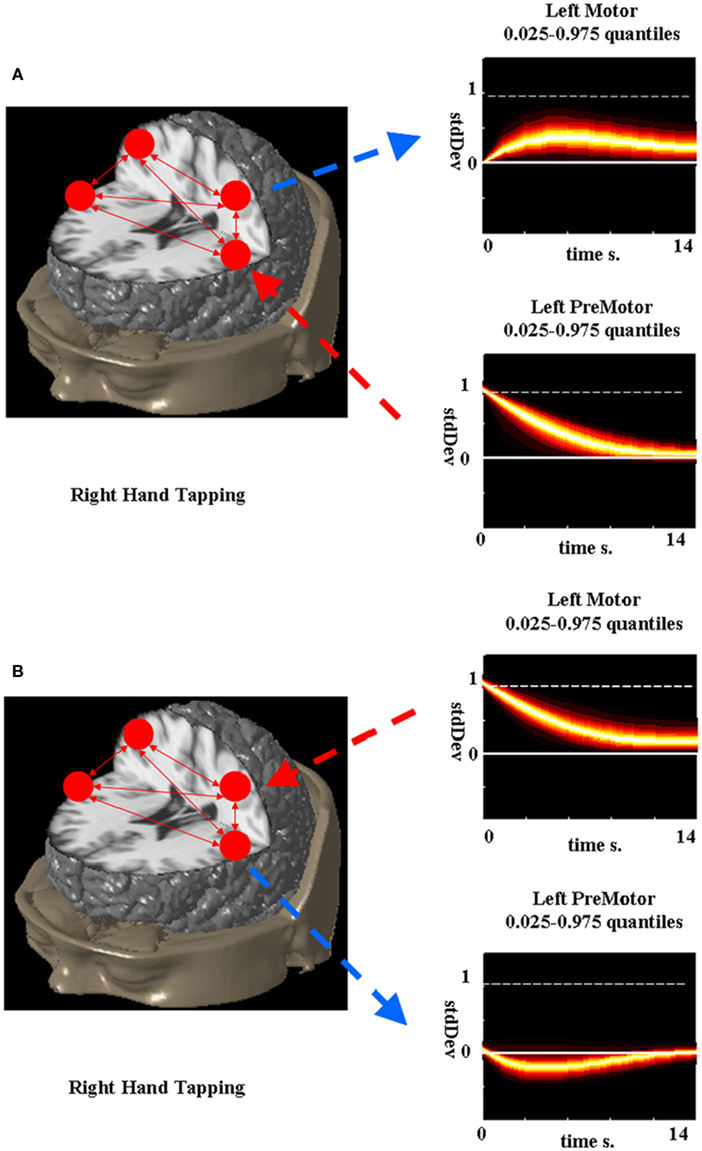
Figure 7. Network impulse response functions for left primary motor and premotor cortex during right hand tapping. Probability density (0.025–0.975) estimated via bootstrap is color-coded for each response function. A 1 SD impulse to the premotor cortex causes a small but sustained increase in the motor cortex while a 1 SD impulse to the primary motor cortex causes a smaller, less sustained decrease in the premotor cortex.

The network impulse responses tell how the changes in modeled quasi-neural activity in a set of regions affect the activity in other modeled regions while performing the modeled task. They can also be extended to estimate the effects of a change in the hemodynamic activity of one region on the neural activity in another region. While useful in understanding network interactions, the impulse response functions are not without problems. First and foremost, they should not be confused with neural impulse response functions as they are not measures of expected neural activity. Rather, they are a tool for analysis of an estimated effective connectivity network. The choice of impulse δ₀ initially added to the network is rather arbitrary and may not reflect a realistic state of the network. The surface validity of orthogonal impulses should be considered (e.g., how likely is driving activity from only one premotor cortex as opposed to both). The network impulse response does provide more information than examination of single parameters and should be calculated prior to interpretation of regional interactions.

Issue Six: Time

The final issue concerns time and its role in causality in fMRI. Essentially this is the question what does an AR or other dynamic model of quasi-neural activity mean when the observations are space 1–0.5 Hz apart? Addressing this issue fully is beyond the scope of the current manuscript. However, several points should be made. Connectivity in LDSf (as well as DCM) is essentially between “deconvolved” fMRI signals temporally localized to individual task conditions and spatially localized to individual brain regions. The goal then is to describe the interactions in a LFP space. However, the fMRI data exists at a sampling rate that is orders of magnitude slower than typically examined with in vivo recordings. Modeled at 0.5 Hz, it is not clear what “quasi-neural interactions” mean. The solution in DCM is to model the fMRI data in continuous time such the interactions between regions are integrated over the time period of an observation. While interactions now occur at intervals more typically associated with LFP, in truth there is no improvement. Such continuous–discrete models (continuous dynamics and discrete observations) must blindly integrate between observation times. Unless the parameters of the dynamic model are well defined a priori, there is no information to constrain them beyond that at the sampling interval. This issue is further compounded by the low-pass filter nature of hemodynamics such that there is limited information even at the sampling interval.

One attractive solution is to combine the high temporal frequency information available in EEG with the high spatial frequency information from fMRI (Horwitz and Poeppel, 2002; Menon and Crottaz-Herbette, 2005; Babajani and Soltanian-Zadeh, 2006; Debener et al., 2006; Ritter and Villringer, 2006; Valdez-Sosa et al., 2008). Both fMRI (Logothetis et al., 2001; Logothetis and Pfeuffer, 2004) and EEG (Steriade, 2001; Niedermeyer and Lopes da Silva, 2004; Freeman et al., 2009) are driven indirectly (fMRI) or directly (EEG) by the dendritic currents responsible for LFPs. This suggests some non-trivial level of agreement can in principle be identified between EEG and fMRI signals. While progress has been made with model driven EEG/fMRI fusion, a biophysical model fully combining the spatial resolution of fMRI and the temporal resolution of EEG remains elusive (Valdez-Sosa et al., 2008). However, data driven (i.e., statistically based) methods have had success (e.g., Martinez-Montes et al., 2004).

As a simplistic demonstration, LDSf model can be augment with a second output matrix to estimate simultaneously recorded EEG data as well as the fMRI data using the same regionally localized quasi-neural hidden states

To illustrate, simultaneous EEG and fMRI data were collected from a single healthy, right-handed subject performing a blocked finger alternation task (Smith et al., 2010). After preprocessing the EEG data to remove artifacts, tensor partial least squares (tPLS) was used to identify EEG electrodes and frequency bands whose weighted combination produced time signatures in hemodynamic space that varied with task condition and were significantly related to fMRI data from brain regions identified as activated by the task (Martinez-Montes et al., 2004) A high beta oscillation centered at 29 Hz was identified with six electrodes participating at statistically significant levels. The fMRI spatial signature of this oscillation included broad areas in the frontal lobes including motor, premotor, and supplementary motor cortex, anterior cingulate, and the head of the caudate nucleus.

The unweighted, unconvolved 29 Hz oscillations from each of these six electrodes were entered into the SLDS model. Eight bilateral regions were selected from the fMRI data based on a separate univariate SPM analysis as well as the tPLS result including primary motor cortices, premotor cortices, two distinct supplementary motor cortex regions, and two distinct anterior cingulate cortex regions. All data were detrended using polynomials up to the third order, centered and normalized to unit variance. The SLDS model was able to identify a single quasi-neural time series from each brain region capable of generating both the observed fMRI and EEG data with considerable accuracy (mean ± SD EEG r = 0.67 ± 0.19, range 0.44–0.90; mean ± SD fMRI r = 0.84 ± 0.09, range 0.71–0.97). LDSf on the fMRI alone also achieved considerable accuracy (mean ± SD fMRI r = 0.82 ± 0.08, range 0.70–0.97). However, the correlation between the estimated quasi-neural time series for each anatomical region from the two models, while statistically significant, was often limited (mean ± SD r = 0.50 ± 0.15, range 0.32–0.74) suggesting different underlying quasi-neural time series were identified by the two models. Statistically combining EEG and fMRI at a quasi-neural level using LDS is a potentially useful means of identifying task related connectivity at a higher temporal resolution than possible with fMRI alone.

The form of fMRI/EEG combination described above is data driven rather than biologically based. The EEG signal is treated more as an aid to the deconvolution of the fMRI signal rather than a signal of interest in its own right. The EEG power data entered into the LDS are a non-linear function (power at 29 Hz/s window) of a linear mixture of signals yet the model treats them as a linear mixture of a non-linear function. Ultimately a biologically justified combination of the two data sets will be needed to produce more meaningful models.

Conclusion

The number of studies utilizing connectivity measures has dramatically increased in recent years (Friston, 2011). However, connectivity methods are still in development; several issues must be addressed to achieve the full utility of these methods. Here we identified six issues with existing connectivity methods we believe are most important. For each problem we provide a possible solution using extensions of the LDSf framework. Considerable future research is needed to validate each of these methodological sketches or incorporate these ideas into other methods. We believe the LDS framework is a promising foundation for effective connectivity analysis.

Conflict of Interest Statement

The authors declare that the research was conducted in the absence of any commercial or financial relationships that could be construed as a potential conflict of interest.

Acknowledgments

This work was supported by the intramural program of the National Institute on Deafness and Other Communication Disorders of the National Institutes of Health. Kewei Chen would also like to acknowledge support from the National Institute on Aging (AG19610 AG025526) and the State of Arizona.

Footnotes

1. ^A recent article by Ramsey et al. (2010) discussed six issues related to causality estimation in fMRI. While similar in spirit and title, the six issues as well as the potential solutions discussed here are distinct from those in Ramsey et al. (2010).
2. ^We use the following standards for equations: Bold face is used for matrices, standard face for vectors, and italic face for scalar values. The tick ′ indicates the transpose of a vector or matrix and a superscript −1 its inverse. P(a|b) indicates the probability of a given b, and N(x, X) indicates a normal distribution with mean x and covariance X with the tilde ~ indicating “distributed as.” E[x] indicates the expected value of x.
3. ^For the regime active at time 1, T_u equals the total observations in the regime −1.
4. ^This fact is not often appreciated. For example in Smith et al. (2011) autoregressive (AR) models are used to estimate connectivity matrices from simulated data generated in continuous time. The discrete AR matrices are then compared to the continuous time matrices without the proper transformations. The AR matrices can contain non-zero elements where the continuous time version is zero and vice-versa. If the continuous time version is held as “ground-truth” the conversion must be calculated prior to comparison.

References

Abarbanel, H. D. I. (1995). Analysis of Observed Chaotic Data. New York: Springer-Verlag.

Abarbanel, H. D. I., Brown, R., Sidorowich, J. J., and Tsimring, L. S. H. (1993). The analysis of observed chaotic data in physical systems. Rev. Mod. Phys. 65, 1331–1392.

CrossRef Full Text

Abler, B., Roebroeck, A., Goebel, R., Hose, A., Schonfeldt-Lecuona, C., Hole, G., and Walter, H. (2006). Investigating directed influences between activated brain areas in a motor-response task using fMRI. Magn. Reson. Imaging 24, 181–185.

Pubmed Abstract | Pubmed Full Text | CrossRef Full Text

Alexander, G. E., and Moeller, J. R. (1994). Application of the scaled subprofile model to functional imaging in neuropsychiatric disorders: a principal component approach to modeling brain function and disease. Hum. Brain Mapp. 2, 79–94.

CrossRef Full Text

Allen, M. R., and Smith, L. A. (1996). Monte Carlo SSA: detecting irregular oscillations in the presence of coloured noise. J. Clim. 9, 3373–3404.

CrossRef Full Text

Andersen, A. H., Gash, D. M., and Avison, M. J. (1999). Principal component analysis of the dynamic response measured by fMRI: a generalized linear systems framework. Magn. Reson. Imaging 17, 795–815.

Pubmed Abstract | Pubmed Full Text | CrossRef Full Text

Babajani, A., and Soltanian-Zadeh, H. (2006). Integrated MEG/EEG and fMRI model based on neural masses. IEEE Trans. Biomed. Eng. 53, 1794–1801.

Pubmed Abstract | Pubmed Full Text | CrossRef Full Text

Barber, D. (2006). Expectation correction for smoothed inference in switching linear dynamical systems. J. Mach. Learn. Res. 7, 2515–2540.

Bar-Shalom, Y., Li, X. R., and Kirubarajan, T. (2001). Estimation with Applications to Tracking and Navigation. New York: John Wiley and Sons.

Beal, M. J., and Ghahramani, Z. (2001). The Variational Kalman Smoother. Gatsby Unit Technical Report TR01-003, University College London, London.

Benkwitz, A., Lütkepohl, H., and Neumann, M. H. (2000). Problems relates to bootstrapping impulse responses of autoregressive processes. Econom. Rev. 19, 69–103.

CrossRef Full Text

Broomhead, D. S., and King, G. P. (1986). Extracting qualitative dynamics from experimental data. Physica D 20 217–236.

CrossRef Full Text

Buchel, C., and Friston, K. J. (1997). Modulation of connectivity in visual pathways by attention: cortical interactions evaluated with structural equation modeling and fMRI. Cereb. Cortex 7, 768–778.

Pubmed Abstract | Pubmed Full Text | CrossRef Full Text

Bullmore, E. T., Rabe-Hesketh, S., Morris, R. G., Williams, S. C. R., Gregory, L., Gray, J. A., and Brammer, M. J. (1996). Functional magnetic resonance image analysis of a large-scale neurocognitive network. Neuroimage 4, 16–23.

Pubmed Abstract | Pubmed Full Text | CrossRef Full Text

Bullmore, E. T., and Sporns, O. (2009). Complex brain networks: graph-theoretical analysis of structural and functional systems. Nat. Rev. Neurosci. 10, 186–198.

Pubmed Abstract | Pubmed Full Text | CrossRef Full Text

Buracas, G. T., Zador, A. M., DeWeese, M. R., and Albright, T. D. (1998). Efficient discrimination of temporal patterns by motion-sensitive neurons in primate visual cortex. Neuron 20, 959–969.

Pubmed Abstract | Pubmed Full Text | CrossRef Full Text

Cheng, B., and Tong, H. (1992). Nonparametric order determination and chaos. J. R. Stat. Soc. B Stat. Methodol. 54, 427–449.

Cole, D. M., Smith, S. M., and Beckmann, C. F. (2010). Advances and pitfalls in the analysis and interpretation of resting state data. Front. Syst. Neurosci. 4:8. doi:10.3389/fnsys.2010.00008

CrossRef Full Text

Cox, H. (1964). On the estimation of state variables and parameters for noisy dynamic systems. IEEE Trans. Automat. Contr. 9, 5–12.

CrossRef Full Text

Debener, S., Ullsperger, M., Siegel, M., and Engel, A. K. (2006). Single-trial EEG-fMRI reveals the dynamics of cognitive function. Trends Cogn. Sci. (Regul. Ed.) 10, 558–563.

Pubmed Abstract | Pubmed Full Text | CrossRef Full Text

Deleus, F., and Van Hulle, M. M. (2009). A connectivity based method for defining regions-of-interest in fMRI data. IEEE Trans. Image Process. 18, 1760–1771.

Pubmed Abstract | Pubmed Full Text | CrossRef Full Text

Dempster, A. P., Laird, N. M., and Rubin, D. B. (1977). Maximum likelihood from incomplete data via the EM algorithm. J. R. Stat. Soc. B Stat. Methodol. 39, 1–38.

Doucet, A., and Andrieu, C. (2001). Iterative algorithms for state estimation of jump Markov linear systems. IEEE Trans. Signal Process. 49, 1216–1227.

CrossRef Full Text

Fox, M. D., Snyder, A. Z., Zacks, J. M., and Raichle, M. E. (2006). Coherent spontaneous activity accounts for trial-to-trial variability in human evoked brain responses. Nat. Neurosci. 9, 23–25.

Pubmed Abstract | Pubmed Full Text | CrossRef Full Text

Freeman, W. J., Ahlfors, S. P., and Menon, V. (2009). Combining fMRI with EEG and MEG in order to relate patterns of brain activity to cognition. Int. J. Psychophysiol. 73, 43–52.

Pubmed Abstract | Pubmed Full Text | CrossRef Full Text

Friston, K. J. (1994). Functional and effective connectivity in neuroimaging: a synthesis. Hum. Brain Mapp. 2, 56–78.

CrossRef Full Text

Friston, K. J. (2011). Dynamic causal modeling and Granger causality comments on: the identification of interacting networks in the brain using fMRI: model selection, causality and deconvolution. Neuroimage 58, 303–305.

Pubmed Abstract | Pubmed Full Text | CrossRef Full Text

Friston, K. J., Harrison, L., and Penny, W. (2003). Dynamic causal modelling. Neuroimage 19, 1273–1302.

Pubmed Abstract | Pubmed Full Text | CrossRef Full Text

Friston, K. J., Li, B., Daunizeau, J., and Stephan, K. E. (2011). Network discovery with DCM. Neuroimage 56, 1202–1221.

Pubmed Abstract | Pubmed Full Text | CrossRef Full Text

Friston, K. J., Mechelli, A., Turner, R., and Price, C. J. (2000). Nonlinear responses in fMRI: the balloon model Volterra kernels, and other hemodynamics. Neuroimage 4, 466–477.

CrossRef Full Text

Friston, K. J., Rotshtein, P., Geng, J. J., Sterzer, P., and Henson, R. N. (2006). A critique of functional localizers. Neuroimage 30, 1077–1087.

Pubmed Abstract | Pubmed Full Text | CrossRef Full Text

Ge, T., Kendrick, K. M., and Feng, J. (2009). A novel extended Granger causal model approach demonstrates brain hemispheric differences during face recognition learning. PLoS Comput. Biol. 5, e1000570. doi:10.1371/journal.pcbi.1000570

CrossRef Full Text

Ghahramani, Z., and Hinton, G. E. (1996). Parameter Estimation for Linear Dynamic Systems. Technical Report CRG-TR-96-2. Department of Computer Science, University of Toronto, Toronto.

Ghahramani, Z., and Hinton, G. E. (1998). Variational learning for switching state-space models. Neural Comput. 12, 963–996.

Ghil, M., Allen, M. R., Dettinger, M. D., Ide, K., Kondrashov, D., Mann, M. E., Robertson, A. W., Saunders, A., Tian, Y., Varadi, F., and Yiou, P. (2002). Advanced spectral methods for climatic time series. Rev. Geophys. 40, 1-1–1-40.

CrossRef Full Text

Goncalves, M. S., and Hall, D. A. (2003). Connectivity analysis with structural equation modeling: an example of the effects of voxel selection. Neuroimage 20, 1455–1467.

Pubmed Abstract | Pubmed Full Text | CrossRef Full Text

Hamilton, J. D. (1989). A new approach to the economic analysis of nonstationary time series and the business cycle. Econometrica 57, 357–384.

CrossRef Full Text

Harrison, L., Penny, W. D., and Friston, K. (2003). Multivariate autoregressive modeling of fMRI time series. Neuroimage 19, 1477–1491.

Pubmed Abstract | Pubmed Full Text | CrossRef Full Text

Havlicek, M., Friston, K. J., Jan, J., Brazdil, M., and Calhoun, V. D. (2011). Dynamic modeling of neuronal responses in fMRI using cubature Kalman filtering. Neuroimage 15, 2109–2128.

CrossRef Full Text

Havlicek, M., Jan, J., Brazdil, M., and Calhoun, V. D. (2010). Dynamic Granger causality based on Kalman filter for evaluation of functional network connectivity in fMRI data. Neuroimage 53, 65–77.

Pubmed Abstract | Pubmed Full Text | CrossRef Full Text

Haykin, S. (2002). Adaptive Filter Theory, 4 Edn. Upper Saddle River, NJ: Prentice-Hall Inc.

Horwitz, B. (2003). The elusive concept of brain connectivity. NeuroImage 19, 466–470.

Pubmed Abstract | Pubmed Full Text | CrossRef Full Text

Horwitz, B., Grady, C. I., Haxby, J. V., Ungerleider, L. G., Schapiro, M. B., Mishkin, M., and Rapoport, S. I. (1992). Functional associations among posterior extrastriate brain region during object and spatial vision. J. Cogn. Neurosci. 4, 311–322.

CrossRef Full Text

Horwitz, B., and Poeppel, D. (2002). How can EEG/MEG and fMRI/PET data be combined. Hum. Brain Mapp. 17, 1–3.

Pubmed Abstract | Pubmed Full Text | CrossRef Full Text

Horwitz, B., Tagamets, M.-A., and McIntosh, A. R. (1999). Neural modeling, functional brain imaging and cognition. Trends Cogn. Sci. 3, 91–98.

Pubmed Abstract | Pubmed Full Text | CrossRef Full Text

Horwitz, B., Warner, B., Fitzer, J., Tagamets, M. A., Husain, F. T., and Long, T. W. (2005). Investigating the neural basis for functional and effective connectivity: application to fMRI. Philos. Trans. R. Soc. Lond. B Biol. Sci. 360, 1093–1108.

Pubmed Abstract | Pubmed Full Text | CrossRef Full Text

Julier, S. J., Uhlmann, J. K., and Durrant-Whyte, H. F. (1995). “A new approach for filtering nonlinear systems,” in Proceedings of the American Control Conference, Seattle, WA, 3, 1628–1632.

Kilian, L. (1998). Small-sample confidence intervals for impulse response functions. Rev. Econ. Stat. 80, 218–230.

CrossRef Full Text

Kilian, L., and Chang, P. L. (2000). How accurate are confidence intervals for impulse responses in large VAR models? Econ. Lett. 69, 299–307.

CrossRef Full Text

Kim, C.-J. (1994). Dynamic linear models with Markov-switching. J. Econom. 60, 1–22.

CrossRef Full Text

Kim, J., and Horwitz, B. (2009). How well does structural equation modeling reveal abnormal brain anatomical connections? An fMRI simulation study. Neuroimage 45, 1190–1198.

Pubmed Abstract | Pubmed Full Text | CrossRef Full Text

Kimoto, M., and Ghil, M. (1993). Multiple flow regimes in the northern hemisphere winter, part II, sectorial regimes and preferred transitions. J. Atmos. Sci. 50, 2645–2673.

CrossRef Full Text

Liu, J., and Newsome, W. T. (2006). Local field potential in cortical area MT: stimulus tuning and behavioral correlations. J. Neurosci. 26, 7779–7790.

Pubmed Abstract | Pubmed Full Text | CrossRef Full Text

Ljung, L. (1979). Asymptotic behavior of the extended Kalman filter as a parameter estimator for linear systems. IEEE Trans. Automat. Contr. 24, 3–50.

CrossRef Full Text

Ljung, L., and Willis, A. (2010). Issues in sampling and estimating continuous time models with stochastic disturbances. Automatica 46, 925–931.

CrossRef Full Text

Logothetis, N. K. (2008). What we can do and what we cannot do with fMRI. Nature 453, 869–878.

Pubmed Abstract | Pubmed Full Text | CrossRef Full Text

Logothetis, N. K., Pauls, J., Augath, M., Torsten, T., and Oeltermann, A. (2001). Neurophysiological investigation of the basis of the fMRI signal. Nature 412, 150–157.

Pubmed Abstract | Pubmed Full Text | CrossRef Full Text

Logothetis, N. K., and Pfeuffer, J. (2004). On the nature of the BOLD fMRI contrast mechanism. Magn. Reson. Imaging 22, 1517–1531.

Pubmed Abstract | Pubmed Full Text | CrossRef Full Text

Lohmann, G., and Bohn, S. (2002). Using replicator dynamics for analyzing fMRI data of the human brain. IEEE Trans. Med. Imaging 21, 485–492.

Pubmed Abstract | Pubmed Full Text | CrossRef Full Text

Lorenz, E. N. (1963). Deterministic nonperiodic flow. J. Atmos. Sci. 20 130–141.

CrossRef Full Text

Lütkepohl, H. (2006). Structural vector autoregressive analysis for cointegrated variables. All. Stat. Arch. 90 75–88.

Lütkepohl, H. (2007). New Introduction to Multiple Time Series Analysis. Berlin: Springer-Verlag.

Makni, S., Beckmann, C., Smith, S., and Woolrich, M. (2008). Bayesian deconvolution of fMRI data using bilinear dynamic systems. Neuroimage 42, 1381–1396.

Pubmed Abstract | Pubmed Full Text | CrossRef Full Text

Mañé, R. (1981). “On the dimension of the compact invariant sets of certain nonlinear maps,” in Lecture Notes in Mathematics 898, eds D. A. Rand, and L. S. Young (Berlin: Springer), 230–242.

Marrelec, G., and Fransson, P. (2011). Assessing the influence of different ROI selection strategies on functional connectivity analyses of fMRI data acquired during steady-state conditions. PLoS ONE 6, e14788. doi:10.1371/journal.pone.0014788

CrossRef Full Text

Martinez-Montes, E., Valdes-Sosa, P. A., Miwakeichi, F., Goldman, R. I., and Cohen, M. S. (2004). Concurrent EEG/fMRI analysis by multiway partial least squares. Neuroimage 22, 1023–1034.

Pubmed Abstract | Pubmed Full Text | CrossRef Full Text

McIntosh, A. R., Bookstein, F. L., Haxby, J. V., and Grady, C. L. (1996). Spatial pattern analysis of functional brain images using partial least squares. Neuroimage 3, 143–157.

Pubmed Abstract | Pubmed Full Text | CrossRef Full Text

McIntosh, A. R., and Gonzalez-Lima, F. (1992). “The application of structural modeling to metabolic mapping if functional neural systems,” in Advances in Metabolic Mapping Techniques for Brain Imaging of Behavioral and Learning Functions, eds F. Gonzalez-Lima, T. Finkenstadt, and H. Scheich (Dordrecht: Kluwer Academic Publishers), 219–255.

McIntosh, A. R., Grady, C., Ungerleider, L. G., Haxby, J. V., Rapoport, S. I., and Horwitz, B. (1994). Network analysis of cortical visual pathways mapped with PET. J. Neurosci. 14, 655–666.

Pubmed Abstract | Pubmed Full Text

McKeown, M. J., Makeig, S., Brown, G. G., Jung, T. P., Kindermann, S. S., Bell, A. J., and Sejnowski, T. J. (1998). Analysis of fMRI data by blind separation into independent spatial components. Hum. Brain Mapp. 6, 160–188.

Pubmed Abstract | Pubmed Full Text | CrossRef Full Text

Menon, V., and Crottaz-Herbette, S. (2005). Combined EEG and fMRI studies of human brain function. Int. Rev. Neurobiol. 66, 291–321.

Pubmed Abstract | Pubmed Full Text | CrossRef Full Text

Moeller, J. R., and Strother, S. C. (1991). A regional covariance approach to the analysis of functional patterns in positron emission tomographic data. J. Cereb. Blood Flow Metab. 11, A121–A135.

Pubmed Abstract | Pubmed Full Text | CrossRef Full Text

Murphy, K. P. (1998). Switching Kalman Filters. Technical Report, DEC/Compaq. Cambridge: Research Labs.

Nelson, A. T. (2000). Nonlinear Estimation and Modeling of Noisy Time-Series by Dual Kalman Filtering Methods. Ph.D. thesis, Oregon Graduate Institute, Hillsboro, Oregon.

Nelson, L. W., and Stear, E. (1967). The simultaneous on-line estimation of parameters and states in linear systems. IEEE Trans. Automat. Contr. 12, 438–442.

CrossRef Full Text

Niedermeyer, E., and Lopes da Silva, F. H. (2004). “Electroencephalography” in Basic Principles, Clinical Applications and Related Fields, 5th Edn. (Philadelphia: Lippincott Williams and Wilkins).

Oh, S. M., Rehg, J. M., Balch, T., and Dellaert, F. (2005). “Data-driven MCMC for learning and inference in switching linear dynamic systems,” in Proceedings of the 20th AAAI National Conference on AI, Pittsburgh, 944–949.

Packard, N. H., Crutchfield, J. P., Farmer, J. D., and Shaw, R. S. (1980). Geometry from a time series. Phys. Rev. Lett. 45, 712–716.

CrossRef Full Text

Parkhomenko, E., Tritchler, D., and Beyene, J. (2009). Sparse canonical correlation analysis with application to genomic data integration. Stat. Appl. Genet. Mol. Biol. 8. doi:10.2202/1544-6115.1406

CrossRef Full Text

Patel, G. S., and Haykin, S. (2001). “Chaotic dynamics,” in Kalman Filtering and Neural Networks, ed. S. Haykin (New York, NY: John Wiley and Sons), 83, :122.

Penny, W. D., Ghahramani, Z., and Friston, K. J. (2005). Bilinear dynamical systems. Philos. Trans. R. Soc. Lond. B Biol. Sci. 360, 983–993.

Pubmed Abstract | Pubmed Full Text | CrossRef Full Text

Penny, W. D., Stephan, K. E., Daunizeau, J., Rosa, M. J., Friston, K. J., Schofield, T. M., and Leff, A. P. (2010). Comparing families of dynamic causal models. PLoS Comput. Biol. 6, e1000709. doi:10.1371/journal.pcbi.1000709

CrossRef Full Text

Penny, W. D., Stephan, K. E., Mechelli, A., and Friston, K. J. (2004). Comparing dynamic causal models. Neuroimage 22, 1157–1172.

Pubmed Abstract | Pubmed Full Text | CrossRef Full Text

Pessoa, L., Gutierrez, E., Bandettini, P. A., and Ungerleider, L. G. (2002). Neural correlates of visual working memory: fMRI amplitude predicts task performance. Neuron 35, 975–987.

Pubmed Abstract | Pubmed Full Text | CrossRef Full Text

Pessoa, L., and Padmala, S. (2005). Quantitative prediction of perceptual decisions during near-threshold fear detection. Proc. Natl. Acad. Sci. U.S.A. 102, 5612–5617.

Pubmed Abstract | Pubmed Full Text | CrossRef Full Text

Plaut, G., and Vautard, R. (1994). Spells of low-frequency oscillations and weather regimes in the Northern hemisphere. J. Atmos. Sci. 51, 210–236.

CrossRef Full Text

Rajapakse, J. C., and Zhou, J. (2007). Learning effective brain connectivity with dynamic Bayesian networks. Neuroimage 37, 749–760.

Pubmed Abstract | Pubmed Full Text | CrossRef Full Text

Ramsey, J. D., Hanson, S. J., Hanson, C., Halchenko, Y. O., Poldrack, R. A., and Glymour, C. (2010). Six problems for causal inference from fMRI. Neuroimage 49, 1545–1558.

Pubmed Abstract | Pubmed Full Text | CrossRef Full Text

Read, P. L. (1993). Phase portrait reconstruction using multivariate singular systems analysis. Physica D 69, 353–365.

CrossRef Full Text

Ress, D., and Heeger, D. J. (2003). Neuronal correlates of perception in early visual cortex. Nat. Neurosci. 6, 414.

Pubmed Abstract | Pubmed Full Text | CrossRef Full Text

Riera, J. J., Watanabe, J., Kazuki, I., Naoki, M., Aubert, E., Ozaki, T., and Kawashima, R. (2004). A state space model of the hemodynamic approach: nonlinear filtering of BOLD signals. Neuroimage 21, 547–567.

Pubmed Abstract | Pubmed Full Text | CrossRef Full Text

Rissman, J., Gazzaley, A., and D’Esposito, M. (2004). Measuring functional connectivity during distinct stages of a cognitive task. Neuroimage 23, 752–763.

Pubmed Abstract | Pubmed Full Text | CrossRef Full Text

Ritter, P., and Villringer, A. (2006). Simultaneous EEG-fMRI. Neurosci. Biobehav. Rev. 30, 823–838.

Pubmed Abstract | Pubmed Full Text | CrossRef Full Text

Roebroeck, A., Formisano, E., and Goebel, R. (2005). Mapping directed influence over the brain using Granger causality and fMRI. Neuroimage 25, 230–242.

Pubmed Abstract | Pubmed Full Text | CrossRef Full Text

Roebroeck, A., Formisano, E., and Goebel, R. (2011). The identification of interacting networks in the brain using fMRI: model selection, causality and deconvolution. NeuroImage 58, 296–302.

Pubmed Abstract | Pubmed Full Text | CrossRef Full Text

Rowe, J. B. (2010). Connectivity analysis is essential to understand neurological disorders. Front. Syst. Neurosci. 4:144. doi:10.3389/fnsys.2010.00144

CrossRef Full Text

Runkle, D. E. (1987). Vector autoregression and reality. J. Bus. Econ. Stat. 5, 437–442.

CrossRef Full Text

Ryali, S., Supekar, K., Chen, T., and Menon, V. (2011). Multivariate dynamical systems models for estimating causal interactions in fMRI. Neuroimage 54, 807–823.

Pubmed Abstract | Pubmed Full Text | CrossRef Full Text

Sardanyés, J., and Solé, R. V. (2007). Delayed transitions in nonlinear replicator networks: about ghosts and hypercycles. Chaos Solitons Fractals 31, 305–315.

Saxe, R., Brett, M., and Kanwisher, N. (2006). Divide and conquer: a defense of functional localizers. Neuroimage 30, 1088–1096.

Pubmed Abstract | Pubmed Full Text | CrossRef Full Text

Schouten, J. C., Takens, F., and Van den Bleek, C. M. (1994). Estimation of the dimension of a noisy attractor. Phys. Rev. A 33 1134–1140.

Shumway, R. H., and Stoffer, D. S. (1991). Dynamic linear models with switching. J. Am. Stat. Assoc. 86, 763–769.

CrossRef Full Text

Sims, C. A. (1980). Macroeconomics and reality. Econometrica 48, 1–48.

Sims, C. A. (1986). Are Forecasting Models Usable for Policy Analysis? Minneapolis: Quarterly Review Federal Reserve Bank, 2–16.

Sims, C. A., and Zha, T. (1999). Error bands for impulse responses. Econometrica 67, 1113–1155.

CrossRef Full Text

Sims, C. A., and Zha, T. (2006). Were there regime switches in U.S. monetary policy? Am. Econom. Rev. 96, 54–81.

CrossRef Full Text

Smith, J. F., Chen, K., Johnson, S., Morrone-Strupinsky, J., Reiman, E. M., Nelson, A., Moeller, J. R., and Alexander, G. E. (2006). Network analysis of single subject fMRI during a finger opposition task. Neuroimage 32, 325–332.

Pubmed Abstract | Pubmed Full Text | CrossRef Full Text

Smith, J. F., Pillai, A., Chen, K., and Horwitz, B. (2010). Identification and validation of effective connectivity networks in functional magnetic resonance imaging using switching linear dynamic systems. Neuroimage 52, 1027–1040.

Pubmed Abstract | Pubmed Full Text | CrossRef Full Text

Smith, S. M., Miller, K. L., Salimi-Khorshidi, G., Webster, M., Beckmann, C. F., Nichols, T. E., Ramsey, J. D., and Woolrich, M. W. (2011). Network modeling methods for FMRI. NeuroImage 54, 875–891.

Pubmed Abstract | Pubmed Full Text | CrossRef Full Text

Spiridon, M., Fischl, B., and Kanwisher, N. (2005). Location and spatial profile of category specific regions in human extrastriate cortex. Hum. Brain Mapp. 27, 77–89.

CrossRef Full Text

Sporns, O., Honey, C. J., and Kotter, R. (2007). Identification and classification of hubs in brain networks. PLoS ONE 2, e1049. doi:10.1371/journal.pone.0001049

CrossRef Full Text

Stephan, K. E., Penny, W. D., Moran, R. J., den Ouden, H. E. M., Daunizeau, J., and Friston, K. J. (2010). Ten simple rules for dynamic causal modeling. Neuroimage 49, 3099–3109.

Pubmed Abstract | Pubmed Full Text | CrossRef Full Text

Stephan, K. E., Tittgemeyer, M., Knösche, T. R., Moran, R. J., and Friston, K. J. (2009). Tractography-based priors for dynamic causal models. Neuroimage 47, 1628–1638.

Pubmed Abstract | Pubmed Full Text | CrossRef Full Text

Steriade, M. (2001). Impact of network activities on neuronal properties in corticothalamic systems. J. Neurophysiol. 86, 1–39.

Pubmed Abstract | Pubmed Full Text

Takens, F. (1981). “Detecting strange attractors in turbulence,” in Lecture Notes in Mathematics 898, eds D. A. Rand, and L. S. Young (Berlin: Springer), 366–381.

Valdes-Sosa, P. A. (2004). Spatio-temporal autoregressive models defined over brain manifolds. Neuroinformatics 2, 239–250.

Pubmed Abstract | Pubmed Full Text | CrossRef Full Text

Valdes-Sosa, P. A., Roebroeck, A., Daunizeau, J., and Friston, K. (2011). Effective connectivity: influence, causality, and biophysical modeling. Neuroimage 58, 339–361.

Pubmed Abstract | Pubmed Full Text | CrossRef Full Text

Valdes-Sosa, P. A., Sanchez-Bornot, J. M., Lage-Castellanos, A., Vega-Hernandez, M., Bosch-Bayard, J., Melie-Garcia, L., and Canales-Rodrigues, E. (2005). Estimating brain functional connectivity with sparse multivariate autoregression. Philos. Trans. R. Soc. Lond. B Biol. Sci. 360, 969–981.

Pubmed Abstract | Pubmed Full Text | CrossRef Full Text

Valdez-Sosa, P. A., Sanchez-Bornot, J. M., Sotero, R. C., Iturria-Medina, Y., Aleman-Gomez, Y., Bosch-Bayard, J., Carbonell, F., and Ozaki, T. (2008). Model driven EEG/fMRI fusion of brain oscillations. Hum. Brain Mapp. 30, 2701–2721.

CrossRef Full Text

Van Dijk, K. R. A., Hedden, T., Venkataraman, A., Evans, K. C., Lazar, S. W., and Buckner, R. L. (2010). Intrinsic functional connectivity as a tool for human connectomics: theory, properties, and optimization. J. Neurophysiol. 103, 297–321.

Pubmed Abstract | Pubmed Full Text | CrossRef Full Text

Vautard, R., and Ghil, M. (1989). Singular spectrum analysis in nonlinear dynamics, with applications to paleoclimatic time series. Physica D 35, 395–424.

CrossRef Full Text

Wagner, A. D., Desmond, J. E., Glover, G. H., and Gabrieli, J. D. E. (1998). Prefrontal cortex and recognition memory: functional-MRI evidence for context-dependent retrieval processes. Brain 121, 1985–2002.

Pubmed Abstract | Pubmed Full Text | CrossRef Full Text

Wan, E. A., and van der Merwe, R. (2001). “The unscented Kalman filter,” in Kalman Filtering and Neural Networks, ed. S. Hayken (New York: Wiley Publishing), 221–280.

Wan, E. A., van der Merwe, R., and Nelson, A. T. (2000). “Dual estimation and the unscented transformation,” in Advances in Neural Information Processing Systems, eds S. A. Sola, T. K. Leen, and K. R. Muller (Cambridge, MA: MIT Press), 666–672.

Whitney, B. (1936). Differentiable manifolds. Ann. Math. 37 645–680.

CrossRef Full Text