
- Mathematical Sciences Unit, Health and Safety Laboratory, Derbyshire, UK
Physiologically based pharmacokinetic (PBPK) models have a potentially significant role in the development of a reliable predictive toxicity testing strategy. The structure of PBPK models are ideal frameworks into which disparate in vitro and in vivo data can be integrated and utilized to translate information generated, using alternative to animal measures of toxicity and human biological monitoring data, into plausible corresponding exposures. However, these models invariably include the description of well known non-linear biological processes such as, enzyme saturation and interactions between parameters such as, organ mass and body mass. Therefore, an appropriate sensitivity analysis (SA) technique is required which can quantify the influences associated with individual parameters, interactions between parameters and any non-linear processes. In this report we have defined the elements of a workflow for SA of PBPK models that is computationally feasible, accounts for interactions between parameters, and can be displayed in the form of a bar chart and cumulative sum line (Lowry plot), which we believe is intuitive and appropriate for toxicologists, risk assessors, and regulators.
Introduction
Current approaches to testing industrial and agricultural chemicals for potential toxicity in people are inefficient, expensive, and reliant on animal experimentation. As a consequence most chemicals in global commerce today have undergone limited or no safety testing at all (Judson et al., 2009).
Over the last few decades alternative methods of evaluating the toxicological hazard of chemical compounds has focused on the potential of in vitro test systems. These are biological systems of a lower level of organization than a complete organism, e.g., isolated organs, cell cultures, and sub-cellular systems. Whilst these systems have been useful in studying the mechanism(s) of toxic action they have been, and perhaps still are, viewed as an alternative means of studying clinically observable toxicity endpoints (Blaauboer, 2010). More recently, the National Research Council (NRC) report, Toxicity Testing in the Twenty-First Century: a Vision and a strategy proposes an ambitious, long-term approach requiring the development of novel in vitro systems (NRC, 2007). This vision is based upon the growing knowledge and elucidation of interconnected pathways composed of complex biochemical interactions of genes, proteins, and small molecules that maintain normal cellular function, control communication between cells and allow cells to adapt to environmental stressors. “Toxicity pathways” are perturbed cellular-response networks that precede and ultimately lead to overt “apical” toxicity. The novel in vitro systems would allow the evaluation of these perturbations of cellular-response pathways. If adopted, the NRC approach would represent a paradigm shift in toxicology and in human and environmental health risk assessment (RA).
The need for alternative approaches to toxicity testing is clear. Whether this involves the development of “traditional,” direct, one to one replacement of animal tests with in vitro systems or “alternative ways” of doing RA, as envisioned in the NRC report, there is a requirement that is common to both: in vitro–in vivo extrapolation. The ability to translate information generated using alternative systems into a reliable predictive toxicity testing strategy is dependent upon a framework into which disparate data can be integrated and utilized. Physiologically based pharmacokinetic (PBPK) models are ideally suited for this and are now recognized as essential tools in the evaluation of in vitro and structure activity relationship-derived data on dose–response relationships in intact organisms (Blaauboer et al., 1996, 1999; DeJongh et al., 1999; Blaauboer 2001,2002,2003a,2003b,2010; Bouvierd’Yvoire et al., 2007).
A PBPK model is an independent, structural model, comprising compartments that correspond directly and realistically to the organs and tissues of the body (e.g., adipose, brain, gut, heart, kidney, liver, lung, muscle, spleen, skin, and bone) and connected by the cardiovascular system. They are mathematical descriptions of biological systems that are translated into computer code and solved computationally. They are frameworks that can capture our understanding of the science underlying the biological processes that lead to disease. A PBPK model is mechanistic because it is specifically formulated to provide insights into the interaction of a foreign chemical(s) with biological processes thought to govern a biological response(s). The principle application of PBPK models is in the prediction of the appropriate form of the target tissue dose, or dose metric, of the parent chemical or its reactive metabolite(s). The dose metric must capture the critical biochemical steps that lead to an effect. Such mechanisms may take place within any compartment, e.g., blood, organ, or sub-cellular compartment. Use of an appropriate dose metric in chemical RA calculations provides a better basis for relating to the observed toxic effects than the external or administered exposure concentration of the parent chemical (Conolly and Butterworth, 1995; Barton et al., 1998; IGHRC, 1999; Johanson et al., 1999; Andersen, 2003; Clewell and Clewell, 2008; Lipscomb and Poet, 2008). Therefore, PBPK models contain knowledge of the system being studied in the form of dozens of parameters and inputs. However, these parameters and inputs are affected by uncertainties, which affect the output of the model.
Sensitivity analysis (SA) allows the model output uncertainty to be ascribed to the source within the model thereby offering a means of evaluating the consistency between internal model structure and the system it tries to emulate (Campolongo and Saltelli, 1997; Campolongo et al., 1999; Saltelli et al., 2004). The many SA methods that exist for the analysis of complex deterministic models can be grouped into two categories: local or one-at-a-time (OAT) methods that consider sensitivities close to a specific set of input parameter values, and global methods, which calculate the contribution of a parameter over the set of all possible input parameters. In a PBPK modeling context a global method would perturb all organ and tissue masses, blood perfusion rates, metabolic parameters, and partition coefficients (PCs) within plausible ranges. The contribution to model output of any single parameter and/or interactions of multiple parameters, e.g., peak venous blood concentration of parent chemical or urinary metabolite is measured yielding useful quantitative information about the overall relative importance of all model parameters. The most commonly applied global method quantifies the importance of parameters as an exact percentage of the total output variance that each factor (or group of factors) is accounting for. This information may be expressed as a bar or pie chart (Campolongo and Saltelli, 1997; Campolongo et al., 1999; Saltelli et al., 2004; Marino et al., 2008) or by the “Lowry Plot” visualizations developed in this paper. In most cases when SA has been conducted on a PBPK model published in the peer-reviewed literature this has been an OAT. This involves the adjustment of individual model parameters, whilst all other parameters are held constant, and observation of the predicted changes in model output, either at a single time or throughout a time course. The results are usually expressed as normalized sensitivity coefficients (SCs), which are the percentage change in the output produced by a fixed and constant percentage (usually 1%) change in the parameter (Plowchalk et al., 1997).
When trying to establish the contribution of a parameter to model predictions, OAT SA techniques are fairly rapid and simple to implement but can give somewhat misleading results if there are substantial interactions among multiple parameters (Campolongo and Saltelli, 1997; Campolongo et al., 1999; Saltelli et al., 2000b, 2004; Loizou et al., 2008). In a model for rat nasal uptake of vinyl acetate the authors conducted an OAT at several exposure concentrations to address the highly non-linear nature of the model and described the SCs as being concentration dependent (Plowchalk et al., 1997). This is inappropriate since the plausible range of the parameters will typically be much wider than this technique allows (and the uncertainty in the parameters should be represented via a joint probability distribution), and as it is OAT results may be unreliable unless the interactions between parameters are negligible, generally this is not true. PBPK models, more often than not, do describe non-linear processes, such as metabolism, and certainly contain interactions between parameters, e.g., tissue and organ masses and blood perfusion rates are related to body mass and cardiac output, respectively. Very often the purpose of the model is to extrapolate beyond the domain of “observation” used to construct and evaluate the model (Andersen and Krishnan, 1994; Andersen, 2003; Barton et al., 2007, 2009; Chiu et al., 2007; Kirman et al., 2008). These model applications and model behaviors along with input variables that are often affected by uncertainties of different orders of magnitude call for a global SA that is independent from assumptions about the model structure (Campolongo and Saltelli, 1997; Campolongo et al., 1999; Saltelli et al., 2004).
Since we are often interested in concentration-time profiles of xenobiotics in biological systems, here we describe an approach for uncertainty and SA adapted to consider sensitivity indices of PBPK model parameters that vary with time. We propose the elements of a workflow for the application of global SA during PBPK model development and evaluation.
Finally, there is a need to develop increased awareness and confidence in the use of PBPK models. Therefore, an important objective underpinning this work is to remain mindful of the need to develop user-friendly tools that shift the emphasis away from mathematical and programming expertise to the biology underlying RA and to present such information in a manner that is acceptable to toxicologists, risk assessors, and regulators. With the future development of intuitive, user-friendly tools, we believe that the workflow we propose does not require in-depth mathematical expertise and could be undertaken by biological scientists. Mathematical equations are included for the interested reader but may be skipped without diminishing the primary objective of this report and we endeavored to provide examples with clear biological relevance. We hope that this work can make a contribution to the development of good PBPK modeling practice and facilitate the dialog between toxicologists and risk assessors and regulators (Kohn, 1995; Clark et al., 2004; Barton et al., 2007; Chiu et al., 2007; Loizou et al., 2008).
Materials and Methods
The PBPK Model
A human PBPK model describing a bladder compartment to simulate fluctuations in metabolite concentration in urine caused by micturition (Franks et al., 2006), was adapted to study the inhalation pharmacokinetics of m-xylene (Figure 1). Liver, adipose, richly and slowly perfused tissues, and the bladder represents the body. The model parameter abbreviations and point values, which are similar to previous models, are listed in Table 1 along with the ranges used in the SA (Loizou et al., 1999; MacDonald et al., 2002). Exhalation, metabolism, and renal excretion were the routes of elimination. The amount of unbound 3-methylhippuric acid (MHA) the main metabolite of m-xylene in the blood, was assumed to be available for secretion into the renal tubules via glomerular filtration where no re-absorption takes place but passes directly into the urine (Rowland et al., 1973). The amount of MHA delivered to the kidney and appearing in the urine was described by the following equations,
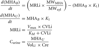
Where, MRLi is the rate of metabolism of m-xylene to MHA in the liver, MWMHA and MWxyl are the molecular weights of MHA and m-xylene, respectively, MHAB is the amount of MHA in the blood, K1 is a first-order elimination rate constant describing removal of MHAB from the blood to the urine, Vmax is the limiting rate and KM is the Michaelis–Menten constant for hepatic metabolism of m-xylene, CVLi is the hepatic venous effluent concentration of m-xylene, MHAU is the amount of MHA in the urine, VolU is the volume of urine in the bladder and Cre is the concentration of creatinine. The concentration of MHA in the urine was expressed in millimole/mole creatinine. To imitate micturition, the bladder is assumed to fill with urine at a constant (but adjustable) rate and empty at discrete time intervals (when the volume of urine reduces to zero). This enables comparison to be made between model predictions and experimental observations with timed sampling in human volunteer studies (Franks et al., 2006).
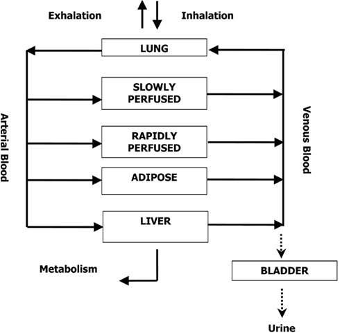
Figure 1. Schematic of the PBPK model for m-xylene.
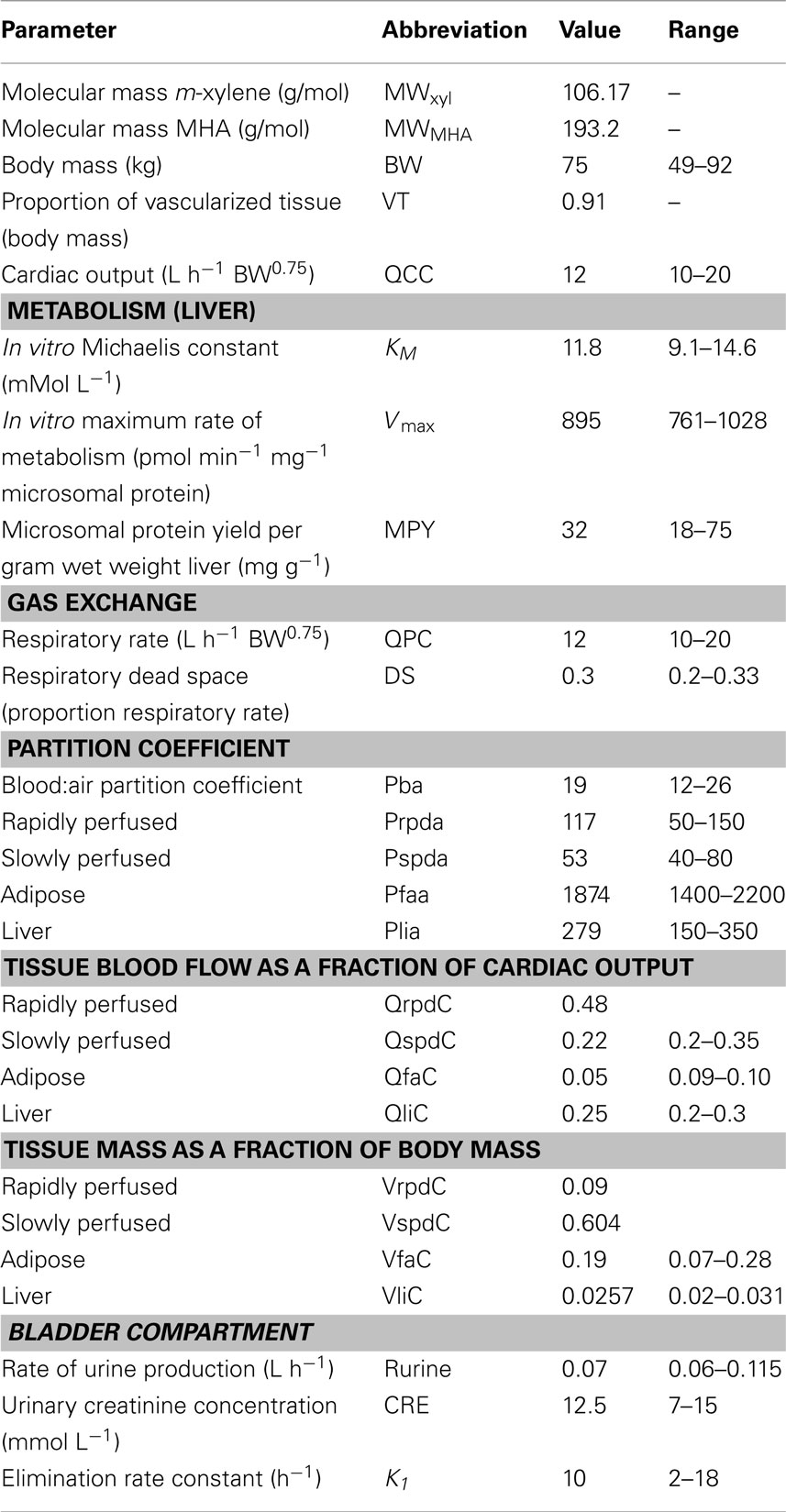
Table 1. Anatomical, physiological, and kinetic constants and parameters used in the PBPK model.
The Michaelis–Menten constant KM and the in vitro Vmax for hepatic metabolism of m-xylene were obtained from the literature (Tassaneeyakul et al., 1996). In vitro –in vivo extrapolation of Vmax was obtained by multiplying the in vitro value by a human hepatic microsomal protein yield (MPY) of 32 mg g−1 wet weight liver and the mass of liver (g) (Howgate et al., 2006; Barter et al., 2007).
Global SA Techniques
The extended Fourier amplitude sensitivity test (eFAST) method proposed in this paper is one of a suite of methods for a quantitative global SA. Alternative model independent methods for calculating main effect and total effect sensitivity indices include the method of Sobol (1993,2001) and the top marginal variances (TMV) method described in Jansen et al. (1994). The Winding Stairs sampling scheme (Chan et al., 2000) is an efficient method of calculating both these sets of sensitivity indices. Indeed, this sampling scheme can also calculate all interaction variances in addition to main and total effects, and can a handle some dependence between inputs. Whilst Sobol’ or TMV have some advantages over eFAST and are suitable alternatives, they require a greater number of model evaluations.
Some alternative methods for a global SA that require many fewer model evaluations are available. These include a class of methods based upon regression analysis (Helton and Davis, 2000) and include standardized regression coefficients (SRC), Spearman correlation coefficients (SCC) and partial correlation coefficients (PCC). These methods are based upon a linear approximation to the model, therefore results from the SA are only approximate and may be poor for highly non-linear models. As the paper proposes a consistent workflow for SA, model dependent methods were considered to be inadequate. Another alternative is an SA method based upon an emulator, a surface fit that approximates the model (Oakley and O’Hagan, 2004). This is a powerful technique, however it requires a greater understanding of the underpinning mathematics (to assess the quality of fit of the emulator) than the method suggested in the paper.
In this study the two-step approach to SA of large models proposed by Campolongo and Saltelli (1997) was adapted for PBPK models as follows:
1. The Morris test as a preliminary screening exercise to identify the subset of the most potentially explanatory parameters of model output.
2. The eFAST for the quantitative analysis of the selected subset of parameters.
The Morris method is global in the sense that it is obtained by taking average values of local measures throughout the input space and produces two sensitivity measures for each parameter, μ and σ. A high μ indicates a factor with an important overall influence on model output; a high σ indicates either a factor interacting with other factors or a factor whose effects are non-linear. The magnitude of μ and σ for each model parameter is relative, i.e., a parameter has a low μ relative to the parameter with the highest μ. For a screening method to be effective, the probability of not identifying a factor that is important must be low. Previous exercises using the Morris method have satisfied this requirement (Campolongo and Saltelli, 1997; Campolongo et al., 1999; Saltelli et al., 2000a).
The eFAST test is a variance-based global method that is independent of any assumptions regarding model structure (it does not rely on assumptions as to the functional relationship between the model output and its inputs) and is valid for use with non-monotonic models (models that do not give exclusively increasing or decreasing predictions). The method provides a way to estimate the expected value and variance of the dose metric (model output variable) and the contribution of input parameters and their interactions to this variance, given physiologically feasible parameter ranges for inputs. It is important that interactions are identified if the applications of SA are to be fully realized (Campolongo and Saltelli, 1997; Campolongo et al., 1999; Saltelli et al., 1999, 2004; Marino et al., 2008). The eFAST technique can produce two types of sensitivity measure that vary with time: main effects (Si) and total effects ( ). The main effect of a parameter represents the reduction in variance if the “true” value of that parameter is known, e.g., the reduction in variation in venous blood concentrations of m-xylene if the real liver mass of an individual is known. The total effect of a parameter represents the proportion of variance remaining if the “true” values of all the other parameters are known, e.g., the variation in venous blood concentrations of m-xylene would be due solely to the variation in liver mass because the true, unique values for all other parameters are known. However, total effects of a given parameter usually have a higher variance when compared to the main effects because although the “true” values of all the other parameters are known, any interactions between these and any number of parameters are unknown. It is useful to think of as the sum of Si and interactions.
SA Workflow
The workflow comprises the following steps:
1. Perform the screening exercise using the Morris test
2. Identify and select the most important parameters
3. Identify the time period where model output variance is of interest
4. Perform eFAST on the most potentially explanatory subset of parameters
5. Present , Si and interactions as a Lowry plot
The Screening Exercise
In order to test the validity of the screening exercise as a single initial step for parameter sensitivity measures that change over time, the means of μ and σ were calculated over a period of 0–14 h corresponding to the change in venous blood concentration of m-xylene (CV; Figure 2A) and from 3 to 14 h corresponding to the change in concentration of urinary MHA (Curine; Figure 2B).
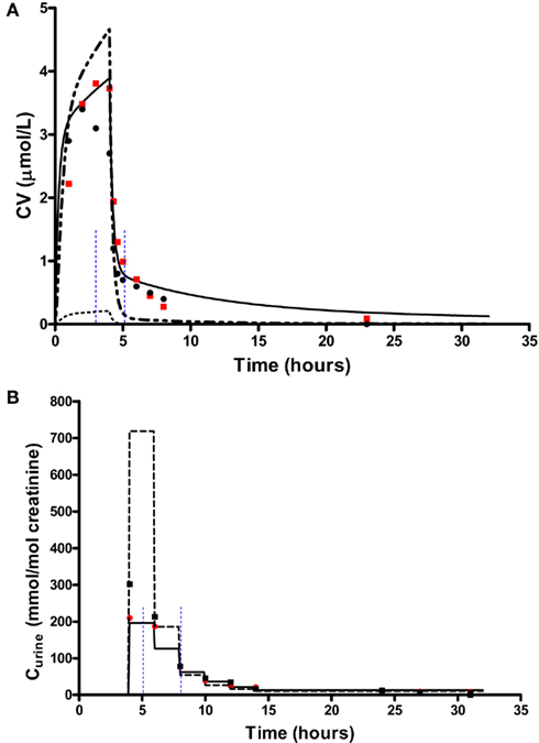
Figure 2. Simulation of venous blood m-xylene and urinary excretion of methylhippuric acid (expressed against creatinine). The symbols are typical measured values from two volunteers and the solid lines are model predictions using mean point values for anatomical, physiological and biochemical parameters for, (A) CV and (B) Curine. In panel (A) the lower broken line shows the region of approximate total variance. The upper broken line is the approximate total variance multiplied by 25 in order to show more clearly the relationship to model prediction. The short broken lines at 3 and 5 h in panel (A) and 5 and 8 h in panel (B) show the time slices chosen for eFAST analysis.
The eFAST Method
In order to delineate the various steps of a possible workflow the analysis initially was conducted at 40 ppm, the target exposure concentration of the human volunteer studies. For CV eFAST was run at 3–5 h, to investigate parameter sensitivities in the distribution and elimination phases (Figure 2A) and at 5–8 h for Curine to investigate the early and latter urinary elimination phase (Figure 2B). In order to investigate parameter interactions further analyses were conducted at 0.3, 3, 5, and 8 h at an intermediate concentration of 200 ppm and at 500 ppm, a concentration calculated to generate a hepatic concentration of m-xylene 17% greater than the KM value for P450 metabolism.
Parameter Ranges
Parameter ranges used for both the Morris Screening and eFAST tests were identical and are listed in Table 1. Anatomical and physiological parameter distributions were obtained from the freely available web-based application PopGen, which is a virtual (healthy) human population generator1. A human population, comprising 50% male and 50% female, white Caucasians, age range 16–65, height range 140–200 cm, body mass indices 18.5–30 was generated to encompass the characteristics of the volunteers that took part in the study described below. In PopGen, organ masses and blood flows are determined for virtual individuals from both a priori distributions of anthropometric parameters such as body mass, height, and body mass index and measured data from existing studies. The algorithms, were derived and evaluated by Willmann et al. (2007).
Parameter ranges were set at the 5 and 95th percentiles of the distributions, with the exceptions of the PCs Prpda, Pspda, Pfaa, and Plia. There were no available distributions for these PCs and therefore the ranges set were considered reasonable assumptions. VspdC and VrpdC, the masses of the slowly and rapidly perfused tissues respectively, were not included in the SA because they are aggregated compartments from which organs and tissues are subtracted when discretely defined during model building. In order to ensure that logical constraints on mass balance and blood flow to the tissues were met the re-parameterizations described in Gelman et al. (1996) were adopted.
The mean value and range for K1, the first-order elimination rate constant describing removal of MHAB from the blood to the urine was estimated by simulating the post exposure urinary excretion of methylhippuric acid following exposures at 1–10, 11–20, 21–30, and 31–40 ppm (Engström et al., 1978). The four data sets from were digitized and K1 estimated using the QuasiNewton algorithm within acslX Libero (see Software).
The Data
Venous blood m-xylene and urinary MHA concentrations from a human volunteer study, which will be fully reported in due course, were used to illustrate the SA analysis workflow. Briefly, groups of four volunteers were exposed for 4 h on two separate occasions to a target concentration of 40 ppm m-xylene vapor in the Health and Safety Laboratory controlled atmosphere facility (CAF), a purpose built room 8 m3 in volume (Loizou et al., 1999). Individual body mass, body fat mass, resting alveolar ventilation rate, blood:air PC, urine volumes, and creatinine concentrations were measured. Venous blood samples were taken prior to entering the exposure facility and at hourly intervals during exposure, then every 20 min for the first hour after exiting the exposure facility before returning to hourly intervals for the next 3 h (Figure 2A). Urine samples were taken at 4, 6, 8, 10, 12, 14, 24, 27, 31 h post exposure (Figure 2B).
Software
The numerical solutions to the model equations were obtained using acslX Libero version 3.0.1.6 (AEgis Technologies2). The M functions for the Morris Test and eFAST included with the acslX Optimum suite of tools were adapted for use in this study. Lowry plots were created using R and ggplot2 (Wickham, 2009; R Development Core Team, 2010) with additional code by Takahashi (2010). Data were digitized using Grab It! Graph Digitizer (Datatrend Software, Inc.3). The computer used in this study was a Dell Optiplex 755 Intel Core(TM)2 Duo CPU 3.00 GHz 2.00 GB RAM.
Results
Results of the Morris screening exercise for variance in CV and Curine are shown in Figures 3A and 3B. The sensitivity indices, μ and σ were plotted for all 19 input parameters but due to lack of space, only 10 in the case of CV, and 7 in the case of Curine, are annotated. The parameters are ranked in order of importance according to μ for both CV and Curine in Table 2. The recommended procedure in Campolongo and Saltelli (1997) would be to perform the more computationally expensive eFAST analysis on the most important of the screened parameters. These would certainly include the annotated parameters in Figures 3A and 3B. However, in this study we investigated the correspondence in ranking of the mean values of μ with eFAST indices for every parameter (no parameters were screened out) for both CV and Curine. Unlike the Morris test mean sensitivity indices, it is not straightforward to take averages of and Si. Therefore, to test concordance with the Morris screening, eFAST was conducted on all 19-model parameters at various discrete time points. The two methods were compared by examining the rankings of the μ and values. Unlike , μ does not include a measure of interactions with other model parameters, therefore strictly speaking, is not a directly comparable sensitivity index. However, since the Morris test has been proposed as a screening method based on ranking μ this comparison is therefore justified (Campolongo and Saltelli, 1997).
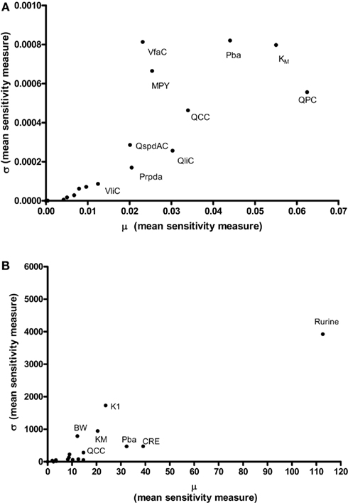
Figure 3. The Morris Screening exercise. Results of the Morris Screening exercise for, (A) the concentration of m-xylene in venous blood (CV) and, (B) the urinary excretion of methylhippuric acid (expressed against creatinine) (Curine).
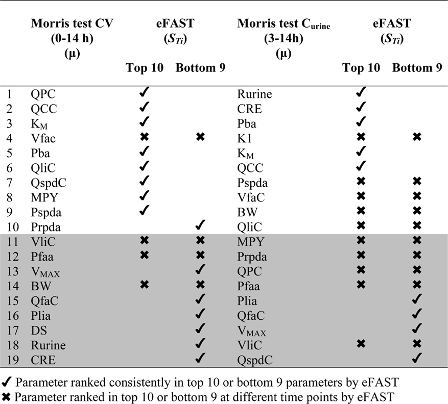
Table 2. Ranking of model parameters: comparison of Morris test screening and eFAST.
Table 2 shows the comparison of ranking of mean values of μ with values calculated at 3, 5, 8, and 11 h for both CV and Curine. A tick next to an value indicates correspondence with the Morris screening across all four time points by being ranked consistently in the top 10 or bottom 9. A cross next to an value indicates a parameter that may be ranked in the top 10 or bottom 9 at different time points.
The Morris screening test was then conducted at the same time points as the eFAST analysis. Tables 3 and 4 show that there is an improved concordance in the ranking between and μ for each parameter at 3, 5, 8, and 11 h for CV but less so for Curine. The rankings are not exactly the same although more parameters are ranked in the top 10 or bottom 9 by both methods. For CV at 3 h BW is ranked in the top 10 most influential parameters and Prpda in the bottom 9 by eFAST in disagreement with the Morris screening. For Curine the following indices differ in ranking to the corresponding μ for VliC and Pspda at 3 h, VliC and K1 at 5 h, VliC, KM, and K1 at 8 h (although K1 was ranked in the top 10 for both methods) and KM and K1 at 11 h.
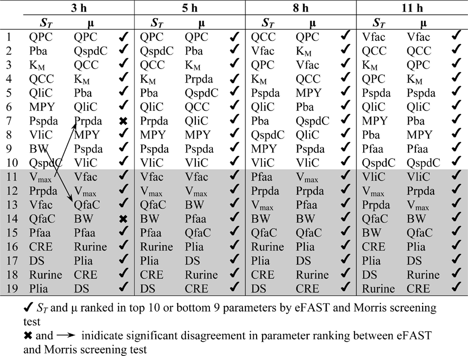
Table 3. Comparison of ranking of model parameters for variance in CV.
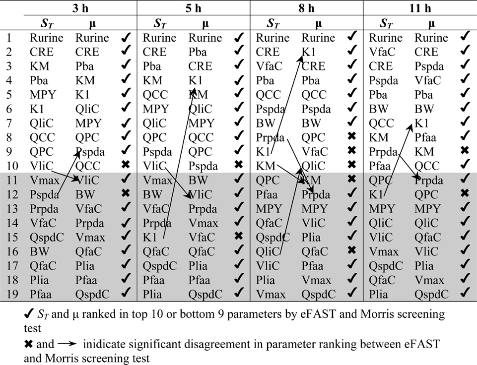
Table 4. Comparison of ranking of model parameters for variance in Curine.
The computing time for the Morris screening test for all 19 parameters for both CV and Curine was approximately 8 s.
The eFAST Method
In addition to calculating and Si eFAST analysis also produces some useful outputs that can be used to support modeling assumptions. The approximate distribution of total variance of the dose metric with time can be visualized to compare with the domain of experimental observation. Figures 2A and 2B show that the magnitude of approximate total variance over time follows the quantity of substance in blood and urine, respectively. In Figure 2A the lower broken line shows the region of approximate total variance for CV. The upper broken line is the approximate total variance multiplied by 25 in order to show more clearly the relationship to model prediction. Therefore, the profile of the approximate total variance of the dose metric was used to select appropriate time points for detailed eFAST analysis. In contrast to CV, the approximate total variance for Curine did not require scaling to be graphed. The figures also highlight that variance is very sensitive to the units of measurement and may be only weakly related to the uncertainty in the level of the substance (in blood, urine, or any body compartment of interest) that arises due to uncertainty in the parameters of the model. This does not impact on the functionality of variance-based methods for SA, however the standard deviation (the square root of the variance) is a more appropriate measure of the underlying uncertainty in the model output that results from parameter value uncertainty. Some outputs in the PBPK model may be much more sensitive to the inputs than others. The total variance can be used to compare the sensitivity of model outputs (to the model inputs) provided those outputs have the same units of measurement. For example, if the variance of the substance in the liver was found to be much larger than the variance of the substance in the kidney, one could conclude that the liver parameter value (e.g., mass, perfusion rate, PC) was a much more sensitive parameter than the corresponding kidney parameter.
Figures 4A,B show the Lowry plots of the eFAST quantitative analysis for CV at 3 and 5 h. Let oi be the main effects (Si), ordered from largest to smallest.
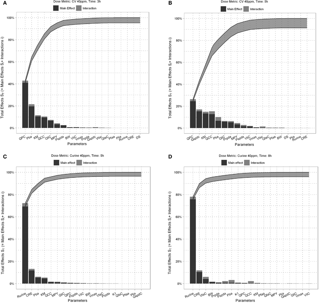
Figure 4. Lowry plot of the eFAST quantitative measure. The total effect of a parameter (), is comprised the main effect Si (black bar) and any interactions with other parameters (grey bar) given as a proportion of variance. The ribbon, representing variance due to parameter interactions, is bounded by the cumulative sum of main effects (lower bold line) and the minimum of the cumulative sum of the total effects (upper bold line), (A) CV at 3 h, (B) CV at 5 h, (C) Curine at 5 h and (D) Curine at 8 h.
The amount of variance that is accounted for by including all parameters up to a specified point is bounded below by the cumulative sum of the ordered main effects (the base of the ribbon) and is bounded above by the cumulative sum of the total effects. Note that there is multiple accounting of the interactions associated with each parameter, which causes the total to exceed 100% eventually. In fact, we have an even stricter limit for the upper bound: it cannot exceed 100% minus the sum of the main effects that are not included in the cumulative sum up to that point (the top of the ribbon).
More formally, the lower bound of the included variance for the first k parameters is given by

and the upper bound is given by
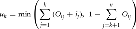
where n is the total number of parameters.
Thus, the amount of variance that is accounted for by including all parameters up to a specified point can be determined by taking a cross section of the ribbon above that parameter, i.e., the range from lk to uk. For example, in Figure 4A, if you include all parameters up to BW, then the amount of variance accounted for is between approximately 94 and 98%. In this case, to ensure that at least 90% of the model variance is captured you would need to include all terms up to and including MPY, since that is the first point when the lower cumulative frequency line rises above 90%. By including the top 10 parameters, we account for between 95% and 99% of variance at 3 h, and between 90 and 98% at 5 h post exposure.
The contribution of different parameters to variance of CV changes with time. The most notable being Qspdc, the blood perfusion rate of the aggregated slowly perfused compartment, which increases from less than 1.0% (Figure 4A) to 15.3% (Figure 4B). The parameters accounting for most of the variance are similar at both time points except that at 5 h body mass, BW is replaced by Pspda, the blood:air PC for the slowly perfused compartment. MPY, can be seen as representing the contribution of Vmax to variance because MPY significantly affects the magnitude of Vmax in the in vitro–in vivo scaling calculation. Therefore, both metabolic parameters, KM and Vmax contribute to variance of CV at both time points.
Figures 4C,D show the results of the eFAST quantitative analysis for Curine at 5 and 8 h. In this case Rurine and CRE are dominant parameters at both time points accounting for about 80–85% variance in Curine. Beyond Rurine and CRE the parameter rankings differ significantly. At 5 h post exposure Rurine, CRE, and Pba, account for at least 86% of variance due the Si and approximately 90% including interactions (Figure 4C). At 8 h post exposure the Si of Rurine, CRE, and VfaC account for at least 90% of variance and almost 95% including interactions (Figure 4D).
Figure 5 is a selection of latticed Lowry plots showing examples of changes in parameter interactions and ordering at various exposure concentrations and time points. There was a broad consistency in the results at the three doses however there were some important differences. The principle differences in results were that (a) the dominance of the most important parameters increased as the dose increased; this was particularly evident at the first two time points (of 0.3 and 3 h) where Pba and QPC accounted for a progressively larger proportion of variance as the dose increased; (b) the results of the SA show that there were some changes in the parameter orderings, in particular MPY became more important as the dose increased; and (c) the Lowry plots clearly indicate that interactions accounted for a larger proportion of variance at all time points for the 200 and 500 ppm doses.
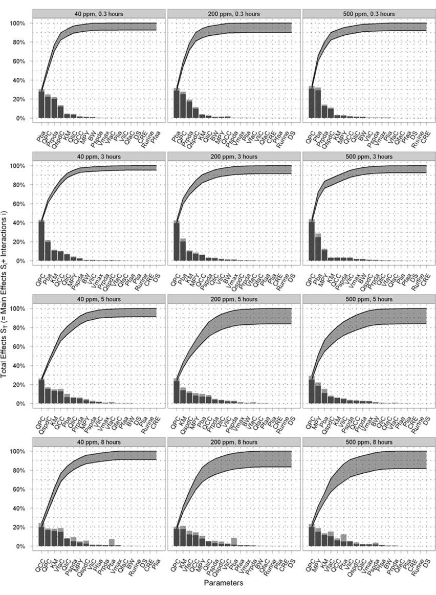
Figure 5. Selected latticed Lowry plots showing concentration and time-dependent changes in parameter interactions and ordering.
The computing time for the eFAST analysis of 19-model parameters for CV and Curine was approximately 13 h each.
Discussion
The probability of non-identification of important parameters by the Morris test has been reported to be low (Campolongo et al., 1999). However, previous studies did not involve the calculation of sensitivity measures that change over time and involved models with a larger number of parameters (60+; Campolongo and Saltelli, 1997; Campolongo et al., 1999; Saltelli et al., 1999; Marino et al., 2008). In this study the Morris screening exercise performed well when conducted at the same time points as eFAST. Disagreement with the Morris screening occurred at the 3-h time point for CV where BW was ranked in the top 10 and Prpda in the bottom 9. Quantitatively, BW accounted for 2.3% and Prpda 0.3% of variance. In the case of Curine disagreement with the Morris screening occurred at each time point. For both CV and Curine the disagreements in rankings were small and occurred with parameters that accounted for a very small percentage of dose metric variance. It is recommended that the screening phase be performed at the same time points as the eFAST analysis.
The computational cost of performing global SA may be an important criterion for determining whether a screening exercise is required. In this study the eFAST conducted on a PBPK model with 19 parameters took approximately 13 h to complete on a dual core desktop PC. However, the run time increases substantially as the number of parameters is increased. In a preliminary investigation the number of model parameters was increased to 25 (each compartment requires a mass, perfusion rate and PC) by adding a kidney and brain compartment. The run time for eFAST analysis of the 25-parameter model increased to 72 h. Therefore, in the case of PBPK models with modest numbers of parameters, e.g., 19–25, the screening should be used to reduce the number of parameters for quantitative analysis by de-selecting the 10 least important. The run time will still be several hours (this would be substantially reduced on a multicore system).
The eFAST results are consistent with other studies showing that the influence of model parameters on model output follow a Pareto-like distribution (Campolongo et al., 1999; Saltelli et al., 2000a). This is a highly skewed distribution with tails corresponding to extreme values. This means that most of the variance would be described by a few parameters. This is certainly the case with the eFAST data obtained at the early time points for both CV and Curine. At 3 and 5 h for CV and 3 and 8 h for Curine, the computation of sensitivity measures occurs in a region of parameter space that corresponds to the time period where the concentration of m-xylene in the system is still substantial. Numerical methods are still able to calculate sensitivity measures even as the variance tends to zero, which occurs at later time points. As this happens the sensitivity measures reflect sampling variability and noise rather than important model structure. It is therefore important to recognize an appropriate point to terminate eFAST, to avoid the region where the variance asymptotes toward zero.
The keys points are that it is important to conduct the SA at a dose within the range of any experimental data as the results from the SA may be sensitive to the dose. However, an advantage of conducting the SA at multiple doses is that the sensitivity of results, in effect the degree of interaction between the parameters of the PBPK model and the dose, can be assessed. Perhaps most importantly, whilst there were some important differences in the most sensitive parameters, there was little change in the ordering of the least important parameters. There was a consistency in the least important parameters at all three doses, therefore the approach suggested in this workflow, of eliminating the least sensitive parameters, was independent of the dose.
The primary objective in the paper was to introduce the elements of a workflow for SA and some of the technical details have been omitted from the methodology for clarity of presentation. One important issue is on the assumed probability distribution for the parameters. In the examples presented in the paper uniform distributions were assumed in all cases. Oakley and O’Hagan (2004) showed that sensitivity indices are influenced by both the relationship between the model output and its inputs, and by the probability distributions for the model parameters. A full treatment of both of these sources of influence is referred to as probabilistic SA. However, this latter source of influence, whilst important, is rarely covered in detail in the literature.
If little information is known about the model parameters it may be reasonable to assume uniform distributions on the inputs (although a robust SA might also examine the results under a variety of assumed probability distributions). However, if it is feasible to obtain reliable probability distributions from sources such as PopGen these should be used in sensitivity analyses. After appropriate transformations of the parameters a variety of distributions can be used in eFAST. Some minor differences in the SA results in this work would have resulted from different probability distributions on the inputs.
In practice there is a balancing act between the availability of a suite of probability distributions and ease of use. The authors consider uniform distributions as a default setting, coupled with a choice of uniform, log-uniform, normal, and log-normal probability distributions for model parameters to be a reasonable compromise.
Despite greater computational cost a number of factors shift the balance in favor of eFAST over OAT techniques. These are: (i) different parameters are affected by different ranges of variation and uncertainty in different regions of parameter space, i.e., different patterns of parameter sensitivity predominate in different regions of parameter space, (ii) the presence of significant interactions between parameters should never be discounted, (iii) presentation of quantitative information on SA in the form of a bar chart is intuitive. Specifically, the presentation of the main effects, Si with a bar representing the sum total contribution of all interactions () to variance in the form of a Lowry plot is recommended, (iv) the importance of one parameter rather than another can only be justified if parameter interactions have been quantified.
Conclusion
We have defined the basis of a workflow for SA of PBPK models that is computationally feasible, accounts for interactions between parameters, and can be displayed in an intuitive manner. When used to analyze PBPK models containing up to 25 parameters, Morris screening should be used to identify the 10 least important. However, judgment and experience should guide the user as to the number of parameters to eliminate before performing the more computationally costly eFAST analysis. The results of eFAST analysis can be presented as a bar chart and cumulative sum line that we have named a “Lowry plot” showing the proportional contribution to variance of the most significant parameters and their interactions. We believe the presentation of this kind of data in this form is intuitive and appropriate for toxicologists, risk assessors and regulators.
Acknowledgments
This work was supported by CEFIC-LRI (Grant No: LRI-B3.7.2-HSLC-081010). The authors thank Conrad Housand and Robin McDougall of The Aegis Technologies Group, Inc for their help in configuring the global sensitivity analysis scripts and for also reviewing the manuscript.
Footnotes
- ^http://xnet.hsl.gov.uk/popgen
- ^http://www.acslx.com/
- ^www.datatrendsoftware.com
References
Andersen, M. E. (2003). Toxicokinetic modeling and its applications in chemical risk assessment. Toxicol. Lett. 138, 9–27.
Andersen, M. E., and Krishnan, K. (1994). Physiologically based pharmacokinetics and cancer risk assessment. Environ. Health Perspect. 102(Suppl. 1), 103–108.
Barter, Z. E., Bayliss, M. K., Beaune, P. H., Boobis, A. R., Carlile, D. J., Edwards, R. J., Houston, J. B., Lake, B. G., Lipscomb, J. C., Pelkonen, O. R., Tucker, G. T., and Rostami-Hodjegan, A. (2007). Scaling factors for the extrapolation of in vivo metabolic drug clearance from in vitro data: reaching a consensus on values of human microsomal protein and hepatocellularity per gram of liver. Curr. Drug Metab. 8, 33–45.
Barton, H. A., Andersen, M. E., and Clewell, H. J. III. (1998). Harmonisation: developing consistent guidelines for applying mode of action and dosimetry information to cancer and noncancer risk assessment. Hum. Ecol. Risk Assess. 4, 74–115.
Barton, H. A., Bessems, J., Bouvier d’Yvoire, M., Buist, H., Clewell, H. III, Gundert-Remy, U., Krishnan, K., Lipscomb, J., Loizou, G., Meek, B., Moir, D., and Spendiff, M. (2009). “Principles of characterizing and applying physiologically-based pharmacokinetic and toxicokinetic models in risk assessment,” in IPCS Project on the Harmonization of Approaches to the Assessment of Risk from Exposure to Chemicals (Geneva: World Health Organization).
Barton, H. A., Chiu, W. A., Setzer, R. W., Andersen, M. E., Bailer, A. J., Bois, F. Y., Dewoskin, R. S., Hays, S., Johanson, G., Jones, N., Loizou, G., Macphail, R. C., Portier, C. J., Spendiff, M., and Tan, Y. M. (2007). Characterizing uncertainty and variability in physiologically-based pharmacokinetic (PBPK) models: state of the science and needs for research and implementation. Toxicol. Sci. 99, 395–402.
Blaauboer, B. J. (2001). Toxicodynamic modelling and the interpretation of in vitro toxicity data. Toxicol. Lett. 120, 111–123.
Blaauboer, B. J. (2002). The necessity of biokinetic information in the interpretation of in vitro toxicity data. Altern. Lab. Anim. 30(Suppl. 2), 85–91.
Blaauboer, B. J. (2003a). Biokinetic and toxicodynamic modelling and its role in toxicological research and risk assessment. Altern. Lab. Anim. 31, 277–281.
Blaauboer, B. J. (2003b). The integration of data on physico-chemical properties, in vitro-derived toxicity data and physiologically based kinetic and dynamic as modelling a tool in hazard and risk assessment. A commentary. Toxicol. Lett. 138, 161–171.
Blaauboer, B. J. (2010). Biokinetic modeling and in vitro-in vivo extrapolations. J. Toxicol. Environ. Health B Crit. Rev. 13, 242–252.
Blaauboer, B. J., Barratt, M. D., and Houston, B. J. (1999). The integrated use of alternative methods in toxicological risk evaluation: ECVAM integrated testing strategies task force report 1. Altern. Lab. Anim. 27, 229–237.
Blaauboer, B. J., Bayliss, M. K., Castell, J. V., Evelo, C. T. A., Frazier, J. M., Groen, K., Gülden, M., Guillouzo, A., Hissink, A. M., Houston, B. J., Johanson, G., de Jongh, J., Kedderis, G. L., Reinhardt, C. A., van de Sandt, J. J. M., and Semino, G. (1996). The use of biokinetics and in vitro methods in toxicological risk evaluation. Altern. Lab. Anim. 24, 473–497.
Bouvier d’Yvoire, M., Prieto, P., Blaauboer, B. J., Bois, F. Y., Boobis, A., Brochot, C., Coecke, S., Freidig, A., Gundert-Remy, U., Hartung, T., Jacobs, M. N., Lavé, T., Leahy, D. E., Lennernäs, H., Loizou, G. D., Meek, B., Pease, C., Rowland, M., Spendiff, M., Yang, J., and Zeilmaker, M. (2007). Physiologically-based kinetic modelling (PBK modelling): meeting the 3Rs agenda: the report and recommendations of ECVAM workshop 63. Altern. Lab. Anim. 35, 661–671.
Campolongo, F., and Saltelli, A. (1997). Sensitivity analysis of an environmental model; a worked application of different analysis methods. Reliab. Eng. Syst. Saf. 57, 49–69.
Campolongo, F., Tarantola, S., and Saltelli, A. (1999). Tackling quantitatively large dimensionality problems. Comput. Phys. Commun. 117, 75–85.
Chan, K., Saltelli, A., and Tarantola, S. (2000). Winding stairs: a sampling tool to compute sensitivity indices. Stat. Comput. 10, 187–196.
Chiu, W. A., Barton, H. A., Dewoskin, R. S., Schlosser, P., Thompson, C. M., Sonawane, B., Lipscomb, J. C., and Krishnan, K. (2007). Evaluation of physiologically based pharmacokinetic models for use in risk assessment. J. Appl. Toxicol. 27, 218–237.
Clark, L. H., Setzer, R. W., and Barton, H. A. (2004). Framework for evaluation of physiologically-based pharmacokinetic models for use in safety or risk assessment. Risk Anal. 24, 1697–1717.
Clewell, R. A., and Clewell, H. J. III. (2008). Development and specification of physiologically based pharmacokinetic models for use in risk assessment. Regul. Toxicol. Pharmacol. 50, 129–143.
Conolly, R. B., and Butterworth, B. E. (1995). Biologically based dose response model for hepatic toxicity: a mechanistically based replacement for traditional estimates of noncancer risk. Toxicol. Lett. 82–83, 901–906.
DeJongh, J., Forsby, A., Houston, J. B., Beckman, M., Combes, R., and Blaauboer, B. J. (1999). An integrated approach to the prediction of systemic toxicity using computer-based biokinetic models and biological in vitro test methods: overview of a prevalidation study based on the ECITTS Project. Toxicol. In vitro 13, 549–554.
Engström, K., Husman, K., Pfäffli, P., and Riihimäki, V. (1978). Evaluation of occupational exposure to xylene by blood, exhaled air and urine analysis. Scand. J. Work Environ. Health 4, 114–121.
Franks, S. J., Spendiff, M. K., Cocker, J., and Loizou, G. D. (2006). Physiologically based pharmacokinetic modelling of human exposure to 2-butoxyethanol. Toxicol. Lett. 162, 164–173.
Gelman, A., Bois, F., and Jiang, J. M. (1996). Physiological pharmacokinetic analysis using population modeling and informative prior distributions. J. Am. Stat. Assoc. 91, 1400–1412.
Helton, J. C., and Davis, F. J. (2000). “Sampling-based methods,” in Sensitivity Analysis, eds A. Saltelli, K. Chan, and E. Scott (London: John Wiley and Sons), 101–152.
Howgate, E. M., Rowland Yeo, K., Proctor, N. J., Tucker, G. T., and Rostami-Hodjegan, A. (2006). Prediction of in vivo drug clearance from in vitro data. I: impact of inter-individual variability. Xenobiotica 36, 473–497.
IGHRC. (1999). Physiologically-Based Pharmacokinetic Modelling: A Potential Tool for Use in Risk Assessment. Institute for Environment and Health, Leicester.
Jansen, M. J. W., Rossing, W. A. H., and Daamen, R. A. (1994). “Monte-Carlo estimation of uncertainty contributions from several independent multi-variate sources,” in Predictability and Nonlinear Modelling in Natural Sciences and Economics, eds J. Gasman, and G. van Straten (Dordrecht: Kluwer Academic Publishers), 334–343.
Johanson, G., Jonsson, F., and Bois, F. (1999). Development of new technique for risk assessment using physiologically based toxicokinetic models. Am. J. Ind. Med. 101–103.
Judson, R., Richard, A., Dix, D. J., Houck, K., Martin, M., Kavlock, R., Dellarco, V., Henry, T., Holderman, T., Sayre, P., Tan, S., Carpenter, T., and Smith, E. (2009). The toxicity data landscape for environmental chemicals. Environ. Health Perspect. 117, 685–695.
Kirman, C. R., Sweeney, L. M., Gargas, M. L., Strother, D. E., Collins, J. J., and Deskin, R. (2008). Derivation of noncancer reference values for acrylonitrile. Risk Anal. 28, 1375–1394.
Lipscomb, J. C., and Poet, T. S. (2008). In vitro measurements of metabolism for application in pharmacokinetic modeling. Pharmacol. Ther. 118, 82–103.
Loizou, G. D., Jones, K., Akrill, P., Dyne, D., and Cocker, J. (1999). Estimation of the dermal absorption of m-xylene vapor in humans using breath sampling and physiologically based pharmacokinetic analysis. Toxicol. Sci. 48, 170–179.
Loizou, G. D., Spendiff, M., Barton, H. A., Bessems, J., Bois, F. Y., Bouvier, d. Y., Buist, H., Clewell, H. III, Gundert-Remy, U., Goerlitz, G., Meek, B., and Schmitt, W. (2008). Development of good modelling practice for physiologically based pharmacokinetic models for use in risk assessment: the first steps. Regul. Toxicol. Pharmacol. 50, 400–411.
MacDonald, A. J., Rostami-Hodjegan, A., Tucker, G. T., and Linkens, D. A. (2002). Analysis of solvent central nervous system toxicity and ethanol interactions using a human population physiologically based kinetic and dynamic model. Regul. Toxicol. Pharmacol. 35, 165–176.
Marino, S., Hogue, I. B., Ray, C. J., and Kirschner, D. E. (2008). A methodology for performing global uncertainty and sensitivity analysis in systems biology. J. Theor. Biol. 254, 178–196.
NRC. (ed.). (2007). Toxicity Testing in the Twenty-First Century: A Vision and a Strategy. Committee on Toxicity and Assessment of Environmental Agents. National Research Council, Washington, DC.
Oakley, J. E., and O’Hagan, A. (2004). Probabilistic sensitivity analysis of complex models: a Bayesian approach. J. R. Stat. Soc. Series B Stat. Methodol. 66, 751–769.
Plowchalk, D. R., Andersen, M. E., and Bogdanffy, M. S. (1997). Physiologically based modeling of vinyl acetate uptake, metabolism, and intracellular pH changes in the rat nasal cavity. Toxicol. Appl. Pharmacol. 142, 386–400.
R Development Core Team. (2010). R: A Language and Environment for Statistical Computing. R Foundation for Statistical Computing, Vienna. Available at: http://www.R-project.org
Rowland, M., Benet, L. Z., and Graham, G. G. (1973). Clearance concepts in pharmacokinetics. J. Pharmacokinet. Biopharm. 1, 123–136.
Saltelli, A., Tarantola, S., and Campolongo, F. (2000b). Sensitivity analysis as an ingredient of modeling. Stat. Sci. 15, 377–395.
Saltelli, A., Tarantola, S., Campolongo, F., and Ratto, M. (2004). Sensitivity Analysis in Practice: A Guide to Assessing Scientific Models. Chichester: John Wiley and Sons Ltd.
Saltelli, A., Tarantola, S., and Chan, K. (1999). A quantitative, model independent method for global sensitivity analysis of model output. Technometrics 41, 39–56.
Sobol, I. M. (1993). Sensitivity estimates for nonlinear mathematical models. Math. Model. Comput. Exp. 1, 407–414.
Sobol, I. M. (2001). Global sensitivity indices for nonlinear mathematical models and their Monte Carlo estimates. Math. Comput. Simul. 55, 271–280.
Takahashi, K. (2010). Build_Legend. Available at: http://tiny.cc/lkl06
Tassaneeyakul, W., Birkett, D. J., Edwards, J. W., Veronese, M. E., Tassaneeyakul, W., Tukey, R. H., and Miners, J. O. (1996). Human cytochrome P450 isoform specificity in the regioselective metabolism of toluene and o-, m- and p-xylene. J. Pharmacol. Exp. Ther. 276, 101–108.
Willmann, S., Hohn, K., Edginton, A., Sevestre, M., Solodenko, J., Weiss, W., Lippert, J., and Schmitt, W. (2007). Development of a physiology-based whole-body population model for assessing the influence of individual variability on the pharmacokinetics of drugs. J. Pharmacokinet. Pharmacodyn. 34, 401–431.
Keywords: PBPK, global sensitivity analysis, alternatives, Lowry plot
Citation: McNally K, Cotton R and Loizou GD (2011) A workflow for global sensitivity analysis of PBPK models. Front. Pharmacol. 2:31. doi: 10.3389/fphar.2011.00031
Received: 08 December 2010; Accepted: 07 June 2011;
Published online: 23 June 2011.
Edited by:
Thomas Hartung, Universität Konstanz, GermanyReviewed by:
Joanna Jaworska, Procter & Gamble, BelgiumMelvin Anderson, The Hamner Institutes for Health Sciences, USA
Copyright: © 2011 McNally, Cotton and Loizou. This is an open-access article subject to a non-exclusive license between the authors and Frontiers Media SA, which permits use, distribution and reproduction in other forums, provided the original authors and source are credited and other Frontiers conditions are complied with.
*Correspondence: George D. Loizou, Mathematical Sciences Unit, Health and Safety Laboratory, Harpur Hill, Buxton, Derbyshire SK17 9JN, UK. e-mail: george.loizou@hsl.gov.uk