Umbral Vade Mecum

1. Introduction

Robust theoretical arguments have established an anticipation of a fundamental minimum measurable length in Nature, of order $L_{\text{Planck}}\equiv \sqrt{\hslash G_N/c^3}=1.6162\times {10}^{-35}\text{m}$, the corresponding mass and time being $M_{\text{Planck}}\equiv \sqrt{\hslash c/G_N}=2.1765\times {10}^{-8}\mathrm{kg}$ and $L_{\text{Planck}}/c=5.3911\times {10}^{-44}\text{s}$. The essence of such arguments is the following (in relativistic quantum geometrical units, wherein ħ, c, and M_Planck are all unity).

In a system or process characterized by energy E, no lengths smaller than L can be measured, where L is the larger of either the Schwarzschild horizon radius of the system (~ E) or, for energies smaller than the Planck mass, the Compton wavelength of the aggregate process (~1/E). Since the minimum of max(E, 1/E) lies at the Planck mass (E = 1), the smallest measurable distance is widely believed to be of order L_Planck. Thus, continuum laws in Nature are expected to be deformed, in principle, by modifications at that minimum length scale.

Remarkably, however, if a fundamental spacetime lattice of spacing a = O(L_PLanck) is the structure that underlies conventional continuum physics, then it turns out that continuous symmetries, such as Galilei or Lorentz invariance, can actually survive unbroken under such a deformation into discreteness, in a non-local, umbral realization (10, 11, 18).

Umbral calculus, pioneered by Rota and associates in a combinatorial context (4, 16), specifies, in principle, how functions of discrete variables in infinite domains provide systematic “shadows” of their familiar continuum limit properties. By preserving Leibniz's chain rule, and by providing a discrete counterpart of the Heisenberg algebra, observables built from difference operators shadow the Lie algebras of the standard differential operators of continuum physics. [For a review relevant to physics, see (13).] Nevertheless, while the continuous symmetries and Lie algebras of umbrally deformed systems might remain identical to their continuum limit, the functions of observables themselves are modified, in general, and often drastically so.

Traditionally, the controlling continuum differential equations of physics are first discretized (2, 5, 18), and then those difference equations are solved to yield umbral deformations of the continuum solutions. But quite often, routine methods to solve such discrete equations become unwieldy, if not intractable. On the other hand, some technical difficulties may be bypassed by directly discretizing the continuum solutions. That is, through appropriate umbral deformation of the continuum solutions, the corresponding discrete difference equations may be automatically solved. However, as illustrated below for the simplest cases of oscillations and wave propagation, the resulting umbral modifications may present some subtleties when it comes to extracting the underlying physics.

In (21) the linearity of the umbral deformation functional was exploited, together with the fact that the umbral image of an exponential is also an exponential, albeit with interesting modifications, to discretize well-behaved functions occurring in solutions of physical differential equations through their Fourier expansion. This discrete shadowing of the Fourier representation functional should thus be of utility in inferring wave disturbance propagation in discrete spacetime lattices. We continue to pursue this idea here with some explicit examples. We do this in conjunction with the umbral deformation of power series, especially those for hypergeometric functions. We compare both Fourier and power series methods in some detail to gain further insight into the umbral framework.

Overall, we utilize essentially all aspects of the elegant umbral calculus to provide systematic solutions of discretized cornerstone differential equations that are ubiquitous in most areas of physics and engineering. We pay particular attention to the umbral counterparts of the Airy, Kummer, and Whittaker equations, and their solutions, and to the umbral maps of solitons for the Sine-Gordon, Korteweg–de Vries, and Toda systems.

2. Overview of the Umbral Correspondence

For simplicity, consider discrete time, t = 0, a, 2a, …, na, …. Without loss of generality, broadly following the summary review of (13), consider an umbral deformation defined by the forward difference discretization of ∂_t,

$\begin{array}{cc}\Delta x(t)\equiv \frac{x(t+a)-x(t)}{a},& (1)\end{array}$

and whence of the elementary oscillation Equation, ẍ(t) = −x(t), namely,

$\begin{array}{cc}{\Delta }^{2}x(t)=\frac{x(t+2a)-2x(t+a)+x(t)}{a^2}=-x(t).& (2)\end{array}$

Now consider the solutions of this second-order difference equation. Of course, (2) can be easily solved directly by the textbook Fourier-component Ansatz x(t) ∝ r^t, (2), to yield (1 ± ia)^t/a. However, to illustrate instead the powerful systematics of umbral calculus (13, 18), we produce and study the solution in that framework.

The umbral framework considers associative chains of operators, generalizing ordinary continuum functions by ultimately acting on a translationally-invariant “vacuum” 1, after manipulations to move shift operators to the right and have them absorbed by that vacuum, which we indicate by T · 1 = 1. Using the standard Lagrange-Boole shift generator

$\begin{array}{cc}\text{}\text{}T\equiv e^{a{\partial }_t},\text{so that}Tf(t)\cdot 1=f(t+a)T\cdot 1=f(t+a),& (3)\end{array}$

the umbral deformation is then

$\begin{array}{cc}{\partial }_t\mapsto \Delta \equiv \frac{T-1}{a},& (4)\end{array}$

$\begin{array}{cc}t\mapsto t{T}^{-1},& (5)\end{array}$

$\begin{array}{cc}{t}^n\mapsto {(t{T}^{-1})}^n=t(t-a)(t-2a)\cdots (t-(n-1)a)T^{-n}\equiv {[t]}^n{T}^{-n},& (6)\end{array}$

so that [t]⁰ = 1, and, for n > 0, [0]ⁿ = 0. The [t]ⁿ are called “basic polynomials”¹ for positive n (5, 13, 16), and they are eigenfunctions of tT⁻¹Δ.

A linear combination of monomials (a power series representation of a function) will thus transform umbrally to the same linear combination of basic polynomials, with the same series coefficients, f(t) ↦ f(tT⁻¹). All observables in the discretized world are thus such deformation maps of the continuum observables, and evaluation of their direct functional form is in order. Below, we will be concluding the correspondence by casually eliminating translation operators at the very end, first through operating on the vacuum and then leaving it implicit, so that F(t) ≡ f(tT⁻¹) · 1.

The umbral deformation relies on the respective umbral entities obeying operator combinatorics identical to their continuum limit (a → 0), by virtue of obeying the same Heisenberg commutation relation (18),

$\begin{array}{cc}[{\partial }_t,t]=1=[\Delta ,t{T}^{-1}].& (7)\end{array}$

Thus, e.g., by shift invariance, TΔT⁻¹ = Δ,

$\begin{array}{cc}[{\partial }_t,t^n]=n{t}^{n-1}\mapsto [\Delta ,{[t]}^n{T}^{-n}]=n{[t]}^{n-1}{T}^{1-n},& (8)\end{array}$

so that, ultimately, Δ[t]ⁿ = n[t]^{n − 1}. For commutators of associative operators, the umbrally deformed Leibniz rule holds (10, 11),

$\begin{array}{cc}[\Delta ,f(t{T}^{-1})g(t{T}^{-1})]=[\Delta ,f(t{T}^{-1})]g(t{T}^{-1})+f(t{T}^{-1})[\Delta ,g(t{T}^{-1})],& (9)\end{array}$

ultimately to be dotted onto 1. Formally, the umbral deformation reflects (unitary) equivalences of the unitary irreducible representation of the Heisenberg-Weyl group, provided for by the Stone-von Neumann theorem. Here, these equivalences reflect the alternate consistent realizations of all continuum physics structures through systematic maps such as the one we have chosen. It is worth stressing that the representations of this algebraic relation on the real or complex number fields can only be infinite dimensional, that is, the lattices covered must be infinite.

Now note that, in this case the basic polynomials [t]ⁿ are just scaled falling factorials, for n ≥ 0, i.e., generalized Pochhammer symbols, which may be expressed in various ways:

$\begin{array}{cc}\begin{array}{l}{[t]}^n\equiv {\left(t{T}^{-1}\right)}^n·1=t(t-a)\cdots (t-\left(n-1\right)a)=a^n\frac{(t/a)!}{(t/a-n)!}\\ =a^n\frac{\Gamma \left(\frac{t}{a}+1\right)}{\Gamma \left(\frac{t}{a}-n+1\right)}={\left(-a\right)}^n\frac{\Gamma \left(n-\frac{t}{a}\right)}{\Gamma \left(-\frac{t}{a}\right)}.\end{array}& (10)\end{array}$

Thus [−t]ⁿ = (−)ⁿ[t + a(n − 1)]ⁿ. Furthermore, [an]ⁿ = aⁿn!; [t]^m[t − am]^{n − m} = [t]ⁿ for 0 ≤ m ≤ n; and for integers 0 ≤ m < n, [am]ⁿ = 0. Thus, Δ^m[t]ⁿ = [an]^m[t]^{n − m}/a^m.

Negative umbral powers, by contrast, are the inverse of rising factorials, instead:

$\begin{array}{cc}\begin{array}{l}{\left[\frac{1}{t}\right]}^n={\left(T\frac{1}{t}\right)}^n\cdot 1=\frac{1}{(t+a)(t+2a)\cdots (t+na)}\\ =a^{-n}\frac{(t/a)!}{(t/a+n)!}\\ =a^{-n}\frac{\Gamma \left(\frac{t}{a}+1\right)}{\Gamma \left(\frac{t}{a}+n+1\right)}={\left(-a\right)}^{-n}\frac{\Gamma \left(-\frac{t}{a}-n\right)}{\Gamma \left(-\frac{t}{a}\right)}.\end{array}& (11)\end{array}$

These correspond to the negative eigenvalues of tT⁻¹Δ.

The standard umbral exponential is then natural to define as (6, 11, 16)²

$\begin{array}{cc}\begin{array}{l}E(\lambda t,\lambda a)\equiv e^{\lambda [t]}\equiv e^{\lambda t{T}^{-1}}\cdot 1={\displaystyle \sum _{n=0}^{\infty }\frac{{\lambda }^n}{n!}{[t]}^n}\\ ={\displaystyle \sum _{n=0}^{\infty }{(\lambda a)}^n\left(\begin{array}{c}t/a\\ n\end{array}\right)={(1+\lambda a)}^{t/a},}\end{array}& (12)\end{array}$

the compound interest formula, with the proper continuum limit (a → 0). N.B. There is always a 0 at λ = −1/a.

Evidently, since Δ · 1 = 0,

$\begin{array}{cc}\Delta e^{\lambda [t]}=\lambda e^{\lambda [t]},& (13)\end{array}$

and, as already indicated, one could have solved this equation directly³ to produce the above E(λt, λa).

Serviceably, the umbral exponential E happens to be an ordinary exponential,

$\begin{array}{cc}{e}^{\lambda [t]}=e^{\frac{\ln (1+\lambda a)}{a}t},& (14)\end{array}$

and it actually serves as the generating function of the umbral basic polynomials,

$\begin{array}{cc}\frac{{\partial }^n}{\partial {\lambda }^n}{(1+\lambda a)}^{t/a}{|}_{\lambda =0}={[t]}^n.& (15)\end{array}$

Conversely, then, this construction may be reversed, by first solving directly for the umbral eigenfunction of Δ, and effectively defining the umbral basic polynomials through the above parametric derivatives, in situations where these might be more involved, as in the next section.

As a consequence of linearity, the umbral deformation of a power series representation of a function is given formally by

$\begin{array}{cc}f(t)\mapsto F(t)\equiv f(t{T}^{-1})·1={f\left(\frac{\partial }{\partial \lambda }\right){(1+\lambda a)}^{t/a}|}_{\lambda =0}.& (16)\end{array}$

This may not always be easy to evaluate, but, in fact, the same argument may be applied to linear combinations of exponentials, and hence the entire Fourier representation functional, to obtain

$\begin{array}{cc}\begin{array}{l}F(t)={\displaystyle {\int }_{-\infty }^{\infty }d}\tau f(\tau ){\displaystyle {\int }_{-\infty }^{\infty }\frac{d\omega }{2\pi }}{e}^{-i\omega \tau }{(1+i\omega a)}^{t/a}\\ ={{\left(1+a\frac{\partial }{\partial \tau }\right)}^{t/a}f(\tau )|}_{\tau =0}.\end{array}& (17)\end{array}$

The rightmost equation follows by converting iω into ∂_τ derivatives and integrating by parts away from the resulting delta function. Naturally, it identifies with Equation (16) by the (Fourier) identity f(∂_x)g(x)|_{x = 0} = g(∂_x)f(x)|_{x = 0}. It is up to individual ingenuity to utilize the form best suited to the particular application at hand.

It is also straightforward to check that this umbral transform functional yields

$\begin{array}{cc}{\partial }_{t}f\mapsto \Delta F,& (18)\end{array}$

and to evaluate the umbral transform of the Dirac delta function, which amounts to a cardinal sine or sampling function,

$\begin{array}{cc}\delta (t)\mapsto \frac{\sin (\frac{\pi }{2}(1+t/a))}{(\pi (a+t))},& (19)\end{array}$

or to evaluate umbral transforms of rational functions, such as

$\begin{array}{cc}f=\frac{1}{(1-t)}\mapsto F=e^{1/a}{a}^{t/a}\Gamma (t/a+1,1/a),& (20)\end{array}$

to obtain an incomplete Gamma function (1), and so on. Note how the last of these is distinctly, if subtly, different from the umbral transform of negative powers, as given in (11).

In practical applications, evaluation of umbral transforms of arbitrary functions of observables may be more direct, at the level of solutions, through this deforming functional, Equation (17). For example, one may evaluate in this way the umbral correspondents of trigonometric functions,

$\begin{array}{cc}\mathrm{Sin}[t]\equiv \frac{e^{i[t]}-e^{-i[t]}}{2i},\mathrm{Cos}[t]\equiv \frac{e^{i[t]}+e^{-i[t]}}{2},& (21)\end{array}$

so that

$\begin{array}{cc}\Delta \mathrm{Sin}[t]=\mathrm{Cos}[t],\Delta \mathrm{Cos}[t]=-\mathrm{Sin}[t].& (22)\end{array}$

As an illustration, consider phase-space rotations of the oscillator. The umbral deformation of phase-space rotations,

$\begin{array}{cc}\dot{x}=p,\dot{p}=-x\mapsto \Delta X(t)=P(t),\Delta P(t)=-X(t),& (23)\end{array}$

readily yields, by directly deforming continuum solutions, the oscillatory solutions,

$\begin{array}{cc}\begin{array}{l}X(t)=X(0)\mathrm{Cos}[t]+P(0)\mathrm{Sin}[t],\\ P(t)=P(0)\mathrm{Cos}[t]-X(0)\mathrm{Sin}[t].\end{array}& (24)\end{array}$

In view of (14), and also

$\begin{array}{cc}(1+ia)=\sqrt{1+a^2}{e}^{i\arctan (a)},& (25)\end{array}$

the umbral sines and cosines in (24) are seen to amount to discrete phase-space spirals,

$\begin{array}{cc}\begin{array}{l}X(t)={(1+a^2)}^{\frac{t}{2a}}(X(0)\cos (\omega t)+P(0)\sin (\omega t)),\\ P(t)={(1+a^2)}^{\frac{t}{2a}}(P(0)\cos (\omega t)-X(0)\sin (\omega t)),\end{array}& (26)\end{array}$

with a frequency decreased from the continuum value (i.e., 1) to

$\begin{array}{cc}\omega =\arctan (a)/a\le 1.& (27)\end{array}$

So the frequency has become, effectively, the inverse of the cardinal tangent function.⁴ Note that the umbrally conserved quantity is,

$\begin{array}{cc}2ℰ=X{(0)}^2+P{(0)}^2={(1+a^2)}^{\frac{-t}{a}}(X{(t)}^2+P{(t)}^2),& (28)\end{array}$

such that $\Delta ℰ=0$, with the proper energy as the continuum limit.

3. Reduction from Second-Order Differences to Single Term Recursions

In this section and the following, to conform to prevalent conventions, the umbral variable will be denoted by x, instead of t. In this case there is a natural way to think of the umbral correspondence that draws on familiar quantum mechanics language (16): The discrete difference equations begin as operator statements, for operator xs and Ts, but are then reduced to equations involving classical-valued functions just by taking the matrix element 〈x|…|vac〉 where |vac〉 is translationally invariant. The overall x-independent non-zero constant 〈x|vac〉 is then ignored.

To be specific, consider Whittaker's equation (1) for μ = 1/2,

$\begin{array}{cc}\left({\partial }_x^2+\frac{\kappa }{x}-\frac{1}{4}\right)y(x)=0.& (29)\end{array}$

This umbrally maps to the operator statement

$\begin{array}{cc}\left({\Delta }^2+T\frac{\kappa }{x}-\frac{1}{4}\right)y(x{T}^{-1})=0.& (30)\end{array}$

Considering either y(xT⁻¹)·1 ≡ Y(x), or else 〈x|y(xT⁻¹)|vac〉 = Y(x) 〈x|vac〉, this operator statement reduces to a classical difference equation,

$\begin{array}{cc}Y(x+2a)-2Y(x+a)+Y(x)+\frac{\kappa a^2}{x+a}Y(x+a)-\frac{a^2}{4}Y(x)=0.& (31)\end{array}$

Before using umbral mapping to convert continuous solutions of (29) into discrete solutions (14, 15) of (31), here we note a simplification of the latter equation upon choosing a = 2, which amounts to setting the scale of x. With this choice (31) collapses to a mere one-term recursion. Shifting x → x − 2 this is

$\begin{array}{cc}Y(x+2)=2\left(\frac{x-2\kappa }{x}\right)Y(x).& (32)\end{array}$

Despite being a first-order difference equation, however, the solutions of this equation still involve two independent “constants of summation” even for x restricted to only integer values, because the choice a = 2 has decoupled adjacent vertical strips of unit width on the complex x plane. To be explicit, for integer x > 0, forward iteration gives (2)

$\begin{array}{ll}\begin{array}{l}Y\left(2k+1\right)=2^k\left({\displaystyle \prod _{j=1}^k\frac{j-2k}{j}}\right)Y(1)\text{ and}\\ Y\left(2k+2\right)=2^k\left({\displaystyle \prod _{j=1}^k\frac{j-k}{j}}\right)Y(2)\text{ for integer }k\ge 0,\end{array}& (33)\end{array}$

with Y(1) and Y(2) the two independent constants that determine values of Y for all larger odd and even integer points, respectively.

Or, if generic x is contemplated, the Equation (32) has elementary solutions, for arbitrary complex constants C₁ and C₂, given by

$\begin{array}{cc}Y(x)=\frac{2^{x/2}\Gamma \left(\frac{x}{2}-\kappa \right)}{\Gamma \left(\frac{x}{2}\right)}{C}_1+\frac{{\left(-2\right)}^{x/2}}{\Gamma \left(\frac{x}{2}\right)\Gamma \left(1-\frac{x}{2}+\kappa \right)} C_2& (34)\end{array}$

$\begin{array}{cc}=\frac{2^{x/2}\Gamma \left(\frac{x}{2}-\kappa \right)}{\Gamma \left(\frac{x}{2}\right)}\left(C_1+\frac{1}{\pi }{\left(-1\right)}^{x/2}{C}_2\sin \pi \left(\frac{x}{2}-\kappa \right)\right).& (35)\end{array}$

In the second expression, we have used Γ(z)Γ(1 − z) = π/sin πz. Note the C₂ part of this elementary solution differs from the C₁ part just through multiplication by a particular complex function with period 2. This is typical of solutions to difference equations since any such periodic factors are transparent to Δ, as mentioned in an earlier footnote (12).

As expected, even for generic x the constants C₁ and C₂ may be determined given Y(x) at two judiciously chosen points, not necessarily differing by an integer. For example, if 0 < κ < 1,

$\begin{array}{cc}{C}_1=\frac{\Gamma (1+\kappa )}{2^{1+\kappa }}Y(2+2\kappa ),C_2=\frac{\pi }{\sin \pi \kappa }{C}_1-\frac{1}{2}\Gamma \left(\kappa \right)Y(2).& (36)\end{array}$

Moreover, poles and zeros of the solution are manifest either from the Γ functions in (34), or else from continued product representations such as (33). For the latter, either forward or backward iterations of the first-order difference Equation (32) may be used. Schematically,

$\begin{array}{cc}Y(x)=\frac{\left(2x-4-4\kappa \right)\left(2x-8-4\kappa \right)\left(2x-12-4\kappa \right)\cdots }{\left(x-2\right)\left(x-4\right)\left(x-6\right)\cdots },& (37)\end{array}$

or alternatively,

$\begin{array}{cc}Y(x)=\frac{x(x+2)(x+4)\cdots }{(2x-4\kappa )(2x+4(1-\kappa ))(2x+4(2-\kappa ))\cdots }.& (38)\end{array}$

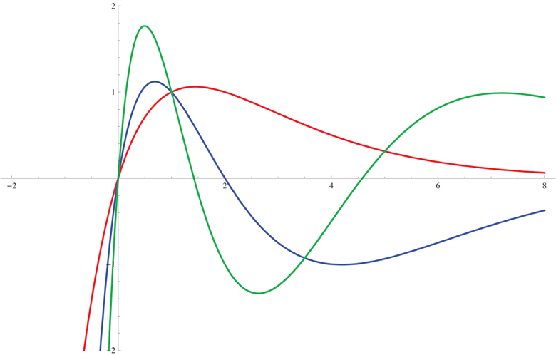
Although both terms in (34) have zeroes, the C₁ term also has poles while the C₂ term has none—it is an entire function of x—and it is complex for any nonzero choice of C₂. Of course, since the Equation (32) is linear, real and imaginary parts may be taken as separate real solutions. All this is evident in the following plots for various selected integer κ.

$\frac{2^{x/2}\Gamma \left(\frac{1}{2}x-\kappa \right)}{\Gamma \left(\frac{1}{2}x\right)}$ for κ = 1, 2, and 3 in red, blue, and green.

$\frac{2^{x/2}\cos \pi \left(\frac{1}{2}x\right)}{\Gamma \left(\frac{1}{2}x\right)\Gamma \left(1-\frac{1}{2}x+\kappa \right)}$ for κ = 1, 2, and 3 in red, blue, and green.

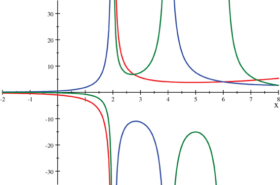
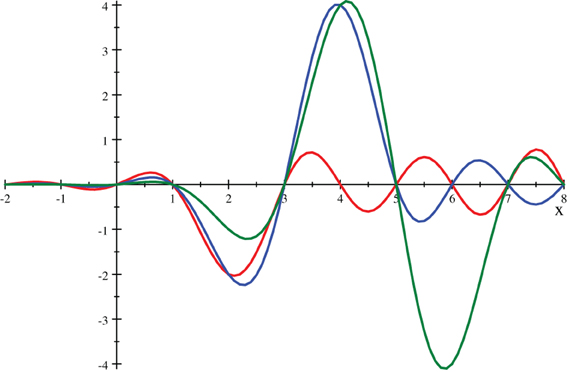
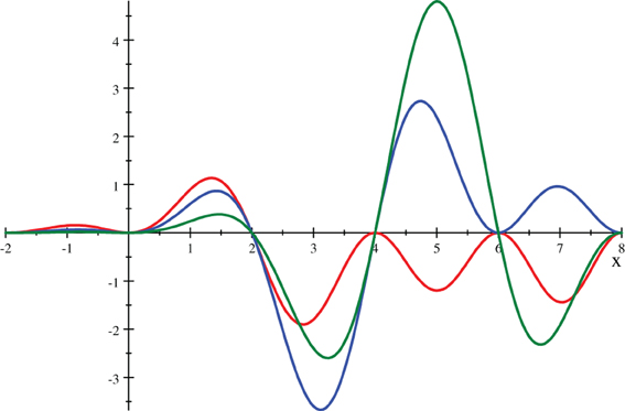
$\frac{2^{x/2}\sin \pi \left(\frac{1}{2}x\right)}{\Gamma \left(\frac{1}{2}x\right)\Gamma \left(1-\frac{1}{2}x+\kappa \right)}$ for κ = 1, 2, and 3 in red, blue, and green.

Collapse to a mere one-term recursion also occurs for an inverse-square potential,

$\begin{array}{cc}\left({\partial }_x^2+\frac{\kappa }{x^2}-\mu \right)y(x)=0.& (39)\end{array}$

For μa² = 1, which amounts to setting the scale of the energy of the solution, the umbral version of this equation reduces to

$\begin{array}{cc}\begin{array}{l}Y(x)=\frac{1}{2}\left(1+\frac{\kappa a^2}{x(x+a)}\right)Y(x+a)\\ =\frac{1}{2}\left(1+\frac{a\kappa }{x}-\frac{a\kappa }{a+x}\right)Y(x+a).\end{array}& (40)\end{array}$

That is to say,

$\begin{array}{cc}Y(x+a)=\frac{2\left(1+\frac{x}{a}\right)\frac{x}{a}}{\left(\frac{x}{a}+\frac{1+\sqrt{1-4\kappa }}{2}\right)\left(\frac{x}{a}+\frac{1-\sqrt{1-4\kappa }}{2}\right)}Y(x).& (41)\end{array}$

Elementary solutions for generic x, for arbitrary complex constants C₁ and C₂, are given by

$\begin{array}{cc}Y(x)=\frac{2^{x/a}}{\Gamma \left(\frac{x}{a}+\frac{1+\sqrt{1-4\kappa }}{2}\right)\Gamma \left(\frac{x}{a}+\frac{1-\sqrt{1-4\kappa }}{2}\right)}\left(\Gamma \left(1+\frac{x}{a}\right)\Gamma \left(\frac{x}{a}\right)C_1+\frac{1}{\Gamma \left(-\frac{x}{a}\right)\Gamma \left(1-\frac{x}{a}\right)}{C}_2\right)& (42)\end{array}$

$\begin{array}{cc}=\frac{2^{x/a}\Gamma \left(1+\frac{x}{a}\right)\Gamma \left(\frac{x}{a}\right)}{\Gamma \left(\frac{x}{a}+\frac{1+\sqrt{1-4\kappa }}{2}\right)\Gamma \left(\frac{x}{a}+\frac{1-\sqrt{1-4\kappa }}{2}\right)}\left(C_1-\frac{1}{{\pi }^2}{C}_2{\sin }^2\left(\frac{\pi x}{a}\right)\right).& (43)\end{array}$

Again, the C₂ part of this elementary solution differs from the C₁ part just through multiplication by a particular complex function with period a. And again, poles and zeros of these and other solutions are manifest either from those of the Γ functions, or else from a continued product form, e.g.

$\begin{array}{cc}Y(x)=\frac{(x^2+xa+\kappa a^2)({(x+a)}^2+(x+a)a+\kappa a^2)\cdots }{(2x(x+a))(2(x+a)(x+2a))\cdots }.& (44)\end{array}$

It is not surprising that (29) and (39) share the privilege to become only first-order difference equations for specific choices of a, as in (32) and (41), because they are both special cases of Whittaker's differential equation, as discussed in the next section. No other linear second-order ODEs lead to umbral equations with this property.

4. Discretization Through Hypergeometric Recursion

In this section we discuss several examples using umbral transform methods to convert solutions of continuum differential equations directly into solutions of the corresponding discretized equations. We use both Fourier and power series umbral transforms.

As an explicit illustration of the umbral transform functional (17), inserting the Fourier representation of the Airy function (1) yields

$\begin{array}{cc}\mathrm{AiryAi}(x)\mapsto \text{UmAiryAi}(x,a)\equiv \mathrm{Re}\left(\frac{1}{\pi }{\displaystyle {\int }_0^{+\infty }{e}^{\frac{1}{3}i{k}^3}}{(1+ika)}^{\frac{x}{a}}dk\right).& (45)\end{array}$

This integral is expressed in terms of hypergeometric functions and evaluated numerically in Appendix A.

Likewise, gaussians also map to hypergeometric functions, as may be obtained by formal series manipulations:

$\begin{array}{cc}\begin{array}{l}{e}^{-x^2}\mapsto G(x,a)\\ \equiv {\displaystyle \sum _{n=0}^{\infty }\frac{{(-)}^n{[x]}^{2n}}{n!}}\\ ={\displaystyle \sum _{n=0}^{\infty }\frac{1}{n!}{(-1)}^n{a}^{2n}\frac{\Gamma \left(\frac{x}{a}+1\right)}{\Gamma \left(\frac{x}{a}-2n+1\right)}}\end{array}& (46)\end{array}$

$\begin{array}{cc}={\displaystyle \sum _{n=0}^{\infty }\frac{\Gamma \left(n-\frac{1}{2}\frac{x}{a}\right)}{\Gamma \left(-\frac{1}{2}\frac{x}{a}\right)}\frac{\Gamma \left(n+\frac{1}{2}-\frac{1}{2}\frac{x}{a}\right)}{\Gamma \left(\frac{1}{2}-\frac{1}{2}\frac{x}{a}\right)}\frac{{\left(-4a^2\right)}^n}{n!}}& (47)\end{array}$

$\begin{array}{cc}{\equiv }_2{}^{F_0}\left(-\frac{1}{2}\frac{x}{a},\frac{1}{2}\left(1-\frac{x}{a}\right);-4a^2\right),& (48)\end{array}$

where the reflection and duplication formulas were used to write

$\begin{array}{cc}\frac{\Gamma \left(\frac{x}{a}+1\right)}{\Gamma \left(\frac{x}{a}-2n+1\right)}=\frac{4^n\Gamma \left(n-\frac{1}{2}\frac{x}{a}\right)\Gamma \left(n+\frac{1}{2}-\frac{1}{2}\frac{x}{a}\right)}{\Gamma \left(-\frac{1}{2}\frac{x}{a}\right)\Gamma \left(\frac{1}{2}-\frac{1}{2}\frac{x}{a}\right)}.& (49)\end{array}$

While the series (47) actually has zero radius of convergence, it is Borel summable, and the resulting regularized hypergeometric function is well-defined. See Appendix B for some related numerics.

For another example drawn from the familiar repertoire of continuum physics, consider the confluent hypergeometric equation of Kummer (A&S 13.1.1):

$\begin{array}{cc}x y^{\prime \prime }+(\beta -x)y^{\prime }-\alpha y=0,& (50)\end{array}$

whose regular solution at x = 0, expressed in various dialects, is

$\begin{array}{cc}y{=}_1{F}_1\left(\alpha ;\beta ;x\right)=M\left(\alpha ,\beta ,x\right)=\mathrm{KummerM}\left(\alpha ,\beta ,x\right),& (51)\end{array}$

with series and integral representations

$\begin{array}{cc}\begin{array}{l}{}_1{F}_1\left(\alpha ;\beta ;x\right)={\displaystyle \sum _{n=0}^{\infty }\frac{\Gamma \left(\alpha +n\right)}{\Gamma \left(\alpha \right)}\frac{\Gamma \left(\beta \right)}{\Gamma \left(\beta +n\right)}\frac{x^n}{n!}}\\ =\frac{\Gamma \left(\beta \right)}{\Gamma \left(\alpha \right)\Gamma \left(\beta -\alpha \right)}{\displaystyle {\int }_0^1{e}^{xs}}{s}^{\alpha -1}{\left(1-s\right)}^{\beta -\alpha -1}ds\\ =1+\frac{\alpha }{\beta }x+\frac{1}{2}\frac{\alpha \left(\alpha +1\right)}{\beta \left(\beta +1\right)}{x}^2+\frac{1}{6}\frac{\alpha \left(\alpha +1\right)\left(\alpha +2\right)}{\beta \left(\beta +1\right)\left(\beta +2\right)}{x}^3+O\left(x^4\right).\end{array}& (52)\end{array}$

The second, independent solution of (50), with branch point at x = 0, is given by Tricomi's confluent hypergeometric function (1), sometimes known as HypergeometricU:

$\begin{array}{cc}U\left(\alpha ,\beta ,x\right)=\frac{\pi }{\sin \pi \beta }\left(\frac{M\left(\alpha ,\beta ,x\right)}{\Gamma \left(1+\alpha -\beta \right)\Gamma \left(\beta \right)}-x^{1-\beta }\frac{M\left(1+\alpha -\beta ,2-\beta ,x\right)}{\Gamma \left(\alpha \right)\Gamma \left(2-\beta \right)}\right).& (53)\end{array}$

Invoking the umbral calculus for x, either of these confluent hypergeometric functions can be mapped onto their umbral counterparts using

$\begin{array}{cc}{}_1{F}_1\left(\alpha ;\beta ;x\right)\mapsto {}_2{F}_1\left(\alpha ,-\frac{x}{a};\beta ;-a\right),& (54)\end{array}$

where ₂F₁ is the well-known Gauss hypergeometric function (1). This map from ₁F₁ to ₂F₁ follows from the basic monomial umbral map,

$\begin{array}{cc}{x}^n\mapsto {[x]}^n\equiv {\left(x{T}^{-1}\right)}^n·1=a^n\frac{\Gamma \left(\frac{x}{a}+1\right)}{\Gamma \left(\frac{x}{a}-n+1\right)}={\left(-a\right)}^n\frac{\Gamma \left(n-\frac{x}{a}\right)}{\Gamma \left(-\frac{x}{a}\right)},& (55)\end{array}$

and from the series (52). When combined, these give the well-known series representation of ₂F₁.

Next, reconsider the one-dimensional Coulomb problem defined by Whittaker's equation for general μ (1):

$\begin{array}{cc}{y}^{\prime \prime }+\left(-\frac{1}{4}+\frac{\kappa }{x}+\frac{\left(\frac{1}{4}-{\mu }^2\right)}{x^2}\right)y=0.& (56)\end{array}$

Since κ and μ are both arbitrary, this also encompasses the inverse-square potential, (39). Exact solutions of this differential equation are

$\begin{array}{cc}y(x)=C_1\mathrm{whittakerM}\left(\kappa ,\mu ,x\right)+C_2\mathrm{whittakerW}\left(\kappa ,\mu ,x\right),& (57)\end{array}$

$\begin{array}{cc}\mathrm{whittakerM}\left(\kappa ,\mu ,x\right)=x^{\mu +1/2}{e}^{-x/2}{}_1{F}_1\text{}\left(\text{}\mu -\kappa +\frac{1}{2};2\mu +1;x\right)\text{},& (58)\end{array}$

$\begin{array}{cc}\begin{array}{l}\mathrm{whittakerW}\left(\kappa ,\mu ,x\right)=x^{\mu +1/2}{e}^{-x/2}\\ \left(\frac{\Gamma \left(-2\mu \right)}{\Gamma \left(-\mu -\kappa +\frac{1}{2}\right)}{}_1{F}_1\left(\mu -\kappa +\frac{1}{2};2\mu +1;x\right)+\frac{\Gamma \left(2\mu \right)}{\Gamma \left(\mu -\kappa +\frac{1}{2}\right)}{x}^{-2\mu }{}_1{F}_1\left(-\mu -\kappa +\frac{1}{2};-2\mu +1;x\right)\right).\end{array}& (59)\end{array}$

Umbral versions of these solutions are complicated by the exponential and overall power factors in the classical relations between the ₁F₁'s and the Whittaker functions, but this complication is manageable. (In part this is because in the umbral calculus there are no ordering ambiguities (20).)

To obtain the umbral version of the Whittaker functions, we begin by evaluating

$\begin{array}{cc}\begin{array}{c}{e}^{-\frac{1}{2}x{T}^{-1}}{}_1{F}_1\left(\alpha ;\beta ;x{T}^{-1}\right)·1={\displaystyle \sum _{m=0}^{\infty }{{\displaystyle \sum _{n=0}^{\infty }\left(-\frac{1}{2}\right)}}^m}\frac{\frac{\Gamma \left(\alpha +n\right)}{\Gamma \left(\alpha \right)}}{\frac{\Gamma \left(\beta +n\right)}{\Gamma \left(\beta \right)}}\frac{{\left[x\right]}^{m+n}}{m!n!}\\ ={\left(1-\frac{a}{2}\right)}^{\frac{x}{a}}{}_2{F}_1\left(\alpha ,-\frac{x}{a};\beta ;\frac{2a}{a-2}\right)\text{},\end{array}& (60)\end{array}$

where we have performed the sum over m first, to obtain

$\begin{array}{cc}{\displaystyle \sum _{m=0}^{\infty }{\left(-\frac{1}{2}\right)}^m}\frac{1}{\Gamma \left(\frac{x}{a}-n-m+1\right)}\frac{a^m}{m!}=\frac{1}{\Gamma \left(\frac{x}{a}-n+1\right)}{\left(1-\frac{a}{2}\right)}^{\frac{x-na}{a}}.& (61)\end{array}$

The sum over n then gives the Gauss hypergeometric function in (60).

Next, to deal with the umbral deformations of the Whittaker functions, we need to use the continuation of (10) and (11) to an arbitrary power of xT⁻¹, namely,

$\begin{array}{cc}{\left(x{T}^{-1}\right)}^{\gamma }=a^{\gamma }\frac{\Gamma \left(\frac{x}{a}+1\right)}{\Gamma \left(\frac{x}{a}-\gamma +1\right)}{T}^{-\gamma }.& (62)\end{array}$

This continuation leads to the following:

$\begin{array}{cc}\begin{array}{l}{\left(x{T}^{-1}\right)}^{\gamma }{e}^{-\frac{1}{2}x{T}^{-1}}{}_1{F}_1\left(\alpha ;\beta ;x{T}^{-1}\right)·1\\ =a^{\gamma }\frac{\Gamma \left(\frac{x}{a}+1\right)}{\Gamma \left(\frac{x}{a}-\gamma +1\right)}{T}^{-\gamma }{e}^{-\frac{1}{2}x{T}^{-1}}{}_1{F}_1\left(\alpha ;\beta ;x{T}^{-1}\right)·1\\ =a^{\gamma }\frac{\Gamma \left(\frac{x}{a}+1\right)}{\Gamma \left(\frac{x}{a}-\gamma +1\right)}{e}^{-\frac{1}{2}\left(x-\gamma a\right)T^{-1}}{}_1{F}_1\left(\alpha ;\beta ;\left(x-\gamma a\right)T^{-1}\right)·1.\end{array}& (63)\end{array}$

Thus we obtain the umbral map

$\begin{array}{cc}{x}^{\gamma }{e}^{-\frac{1}{2}x}{}_1{F}_1\left(\alpha ;\beta ;x\right)\mapsto \frac{\Gamma \left(\frac{x}{a}+1\right)}{\Gamma \left(\frac{x}{a}-\gamma +1\right)} a^{\gamma }{\left(1-\frac{a}{2}\right)}^{\frac{x}{a}-\gamma }{}_2{F}_1\left(\alpha ,\gamma -\frac{x}{a};\beta ;\frac{2a}{a-2}\right).& (64)\end{array}$

Finally then, specializing to the relevant α, β, and γ, we find the umbral Whittaker functions. In particular,

$\begin{array}{cc}\begin{array}{c}\mathrm{whittakerM}\left(\kappa ,\mu ,x\right)\mapsto \frac{\Gamma \left(\frac{x}{a}+1\right)}{\Gamma \left(\frac{x}{a}-\mu +\frac{1}{2}\right)}{a}^{\mu +1/2}{\left(1-\frac{a}{2}\right)}^{\frac{x}{a}-\mu -\frac{1}{2}}\\ {}_2{F}_1\left(\mu +\frac{1}{2}-\kappa ,\mu +\frac{1}{2}-\frac{x}{a};2\mu +1;\frac{2a}{a-2}\right).\end{array}& (65)\end{array}$

This result for general a exhibits what is special about the choice a = 2, as exploited in the previous section. To realize that choice from (65) requires taking a limit a ↗ 2, hence it requires the asymptotic behavior of the Gauss hypergeometric function (1):

$\begin{array}{cc}{}_2{F}_1\left(\alpha ,\beta ;\gamma ;z\right)\underset{z\to -\infty }{~}\frac{\Gamma \left(\gamma \right)}{\Gamma \left(\beta \right)}\frac{\Gamma \left(\beta -\alpha \right)}{\Gamma \left(\gamma -\alpha \right)}{\left(-z\right)}^{-\alpha }+\frac{\Gamma \left(\gamma \right)}{\Gamma \left(\alpha \right)}\frac{\Gamma \left(\alpha -\beta \right)}{\Gamma \left(\gamma -\beta \right)}{\left(-z\right)}^{-\beta }.\text{}\text{}\text{}\text{}& (66)\end{array}$

Now with sufficient care, a = 2 solutions can be coaxed from the umbral version of whittakerM in (65), and/or the corresponding umbral counterpart of whittakerW, upon taking lim_a↗2 and making use of (66). Moreover, in principle the umbral correspondents of both Whittaker functions could be used to obtain from this limit a solution with two arbitrary constants.

On the other hand, for a = 2, the umbral equation corresponding to (56) again reduces to a one-term recursion, namely,

$\begin{array}{cc}Y(x+2)=\frac{2\left(x+2\right)\left(x-2\kappa \right)}{\left(x+1+2\mu \right)\left(x+1-2\mu \right)}Y(x).& (67)\end{array}$

For generic x, solutions for arbitrary complex constants C₁ and C₂ are then given by

$\begin{array}{cc}Y(x)=\frac{2^{x/2}}{\Gamma \left(\frac{x}{2}+\frac{1}{2}+\mu \right)\Gamma \left(\frac{x}{2}+\frac{1}{2}-\mu \right)}\left(\Gamma \left(1+\frac{x}{2}\right)\Gamma \left(\frac{x}{2}-\kappa \right)C_1+\frac{1}{\Gamma \left(-\frac{x}{2}\right)\Gamma \left(1+\kappa -\frac{x}{2}\right)}{C}_2\right)& (68)\end{array}$

$\begin{array}{cc}=\frac{2^{x/2}\Gamma \left(1+\frac{x}{2}\right)\Gamma \left(\frac{x}{2}-\kappa \right)}{\Gamma \left(\frac{x}{2}+\frac{1}{2}+\mu \right)\Gamma \left(\frac{x}{2}+\frac{1}{2}-\mu \right)}\left(C_1+\frac{1}{{\pi }^2} C_2\sin \left(\frac{\pi x}{2}\right)\sin \pi \left(\frac{x}{2}-\kappa \right)\right),& (69)\end{array}$

which agrees with (34) when μ = 1/2, of course. As in that previous special case, the C₂ part of (68) differs from the C₁ part just through multiplication by a particular complex function with period 2 (12).

We graph some examples to show the differences between the Whittaker functions and their umbral counterparts, for a = 1.

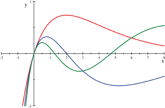
whittakerM(κ, 1/2, x) for κ = 1, 2, and 3 in red, blue, and green.

Umbral whittakerM(κ, 1/2, x) for a = 1, and for κ = 1, 2, and 3 in red, blue, and green.

The examples above are specific illustrations of combinatorics that may be summarized in a few umbral hypergeometric mapping lemmata, the simplest being

Lemma 1:

$\begin{array}{cc}{}_p{F}_q({\alpha }_1,\dots ,{\alpha }_p;{\beta }_1,\dots ,{\beta }_q;x){\mapsto }_{p+1}{F}_q({\alpha }_1,\dots ,{\alpha }_p,-x/a;{\beta }_1,\dots ,{\beta }_q;-a),& (70)\end{array}$

where the series representation of the generalized hypergeometric function _pF_q is⁵

$\begin{array}{cc}{}_p{F}_q\left({\alpha }_1,\dots ,{\alpha }_p;{\beta }_1,\dots ,{\beta }_q;x\right)\text{}\text{}\text{}\text{}=\frac{\Gamma \left({\beta }_1\right)\cdots \Gamma \left({\beta }_q\right)}{\Gamma \left({\alpha }_1\right)\cdots \Gamma \left({\alpha }_p\right)}{\displaystyle \sum _{n=0}^{\infty }\frac{\Gamma \left({\alpha }_1+n\right)\cdots \Gamma \left({\alpha }_p+n\right)}{\Gamma \left({\beta }_1+n\right)\cdots \Gamma \left({\beta }_q+n\right)}}\frac{x^n}{n!}.& (71)\end{array}$

A proof of (70) follows from formal manipulations of these series.

The umbral version of a more general class of functions is obtained by replacing x → xT⁻¹ in functions of x^k for some fixed positive integer k. Thus, again for hypergeometric functions, we have

Lemma 2:

$\begin{array}{cc}\begin{array}{l}{}_p{F}_q\left({\alpha }_1,\dots ,{\alpha }_p;{\beta }_1,\dots ,{\beta }_q;x^k\right)\mapsto \\ {}_{p+k}{F}_q({\alpha }_1,\dots ,{\alpha }_p,\frac{1}{k}\left(-\frac{x}{a}\right),\frac{1}{k}\left(1-\frac{x}{a}\right),\dots ,\frac{1}{k}\left(k-1-\frac{x}{a}\right);{\beta }_1,\dots ,{\beta }_q;{\left(-ak\right)}^k).\end{array}& (72)\end{array}$

And again, a proof follows from formal series expansions.

Multiplication by exponentials produces only minor modifications of these general results, as was discussed above in the context of Whittaker functions, namely,

Lemma 3:

$\begin{array}{cc}\begin{array}{l}{e}^{\lambda x}{}_p{F}_q\left({\alpha }_1,\dots ,{\alpha }_p;{\beta }_1,\dots ,{\beta }_q;x^k\right)\mapsto \\ {\left(1+a\lambda \right)}^{\frac{x}{a}}{}_{p+k}{F}_q({\alpha }_1,\dots ,{\alpha }_p,\frac{1}{k}\left(-\frac{x}{a}\right),\frac{1}{k}\left(1-\frac{x}{a}\right),\dots ,\frac{1}{k}\left(k-1-\frac{x}{a}\right);{\beta }_1,\dots ,{\beta }_q;{\left(\frac{-ak}{1+a\lambda }\right)}^k).\end{array}& (73)\end{array}$

In addition, multiplication by an overall power of x gives

Lemma 4:

$\begin{array}{cc}\begin{array}{l}{x}^{\gamma }{e}^{\lambda x}{}_p{F}_q\left({\alpha }_1,\dots ,{\alpha }_p;{\beta }_1,\dots ,{\beta }_q;x^k\right)\mapsto \\ \frac{\Gamma \left(\frac{x}{a}+1\right)a^{\gamma }{\left(1+a\lambda \right)}^{\frac{x}{a}-\gamma }}{\Gamma \left(\frac{x}{a}-\gamma +1\right)}{}_{p+k}{F}_q({\alpha }_1,\dots ,{\alpha }_p,\frac{\gamma -\frac{x}{a}}{k},\frac{1+\gamma -\frac{x}{a}}{k},\dots ,\frac{k-1+\gamma -\frac{x}{a}}{k};{\beta }_1,\dots ,{\beta }_q;{\left(\frac{-ak}{1+a\lambda }\right)}^k).\end{array}& (74)\end{array}$

5. Wave Propagation

Given the umbral features of discrete time and space equations discussed above, separately, it is natural to combine the two.

For example, the umbral version of simple plane waves in 1+1 spacetime would obey an equation of the type (6, 11, 12),

$\begin{array}{cc}({\Delta }_x^2-{\Delta }_t^2)F=0,& (75)\end{array}$

on a time-lattice with spacing a and a space-lattice with spacing b, not necessarily such that b = a in all spacetime regions. For generic frequency, wavenumber and velocity, the basic solutions are

$\begin{array}{cc}f=e^{i(\omega t-kx)}\mapsto F={\left(1+i\omega a\right)}^{t/a}{\left(1-ikb\right)}^{x/b}.& (76)\end{array}$

For right-moving waves, say, these have phase velocity

$\begin{array}{cc}v(\omega ,k)=\frac{\omega }{k} \frac{a\arcsin (b)}{b\arcsin (a)}.& (77)\end{array}$

Thus, the effective index of refraction in the discrete medium is (b arcsin(a))/(a arcsin(b)), i.e., modified from 1. Small inhomogeneities of a and b in the fabric of spacetime over large regions could therefore yield interesting effects.

Technically, a more challenging application of umbral methods involves nonlinear, solitonic phenomena (21), such as the one-soliton solution of the continuum Sine-Gordon equation,

$\begin{array}{cc}({\partial }_x^2-{\partial }_t^2)f\left(x,t\right)=\sin (f(x,t)),f_{\text{SG}}(x,t)=4\arctan \left(m{e}^{\frac{x-vt}{\sqrt{1-v^2}}}\right)\text{}.& (78)\end{array}$

The corresponding umbral deformation of the PDE itself would now also involve a deformed potential sin(f(xT⁻¹_x, tT⁻¹_t))·1. But rather than tackling this difficult nonlinear difference equation, one may instead use the umbral transform (17) to infer that f_SG(x, t) maps to

$\begin{array}{cc}{F}_{\text{SG}}\left(a,b;x,t\right)={\displaystyle {\int }_{-\infty }^{\infty }\text{}}\text{}\frac{d\chi d\tau d\omega dk}{{\left(2\pi \right)}^2}4\arctan \left(m{e}^{\frac{\chi -v\tau }{\sqrt{1-v^2}}}\right)e^{ik\chi -i\omega \tau }{\left(1+i\omega a\right)}^{t/a}{\left(1-ikb\right)}^{x/b}.& (79)\end{array}$

The continuum Korteweg–de Vries soliton is likewise mapped:

$\begin{array}{cc}\begin{array}{l}{f}_{\text{KdV}}(x,t)=\frac{v}{2}{\mathrm{sech}}^2\left(\frac{\sqrt{v}}{2}(x-vt)\right)\mapsto \\ F_{\text{KdV}}\left(a,b;x,t\right)={\displaystyle {\int }_{-\infty }^{\infty }\text{}}\text{}\frac{d\chi d\tau d\omega dk}{{\left(2\pi \right)}^2}\frac{v}{2}{\mathrm{sech}}^2\left(\frac{\sqrt{v}}{2}(\chi -v\tau )\right)e^{ik\chi -i\omega \tau }{\left(1+i\omega a\right)}^{t/a}{\left(1-ikb\right)}^{x/b}.\end{array}& (80)\end{array}$

Closed-form evaluations of these Fourier integrals are not available, but the physical effects of the discretization could be investigated numerically, and compared to the Lax pair integrability machinery of (13), or to the results on a variety of discrete KdVs in (17), or to other studies (8, 9).

However, a more accessible example of umbral effects on solitons may be found in the original Toda lattice model (19). For this model the spatial variable is already discrete, usually with spacing b = 1 so x = n is an integer, while the time t is continuous. The equations of motion in that case are

$\begin{array}{cc}\begin{array}{l}\frac{\partial q\left(n,t\right)}{\partial t}=p\left(n,t\right),\\ \frac{\partial p\left(n,t\right)}{\partial t}=-\left(e^{-\left(q\left(n+1,t\right)-q\left(n,t\right)\right)}-e^{-\left(q\left(n,t\right)-q\left(n-1,t\right)\right)}\right),\end{array}& (81)\end{array}$

for integer n. Though x = n is discrete, nevertheless there are exact multi-soliton solutions valid for all continuous t, as is well-known.

Specific one-soliton Toda solutions are given for constant α, β, γ, and q₀ by

$\begin{array}{cc}q\left(n,t\right)=q_0+\log \left(\frac{1+\alpha \exp \left(-\beta n+\gamma t\right)}{1+\alpha \exp \left(-\beta \left(n+1\right)+\gamma t\right)}\right),& (82)\end{array}$

$\begin{array}{cc}p\left(n,t\right)=\alpha \gamma \left(\frac{e^{-n\beta +\gamma t}}{\alpha e^{-n\beta +\gamma t}+1}-\frac{e^{-\left(n+1\right)\beta +\gamma t}}{\alpha e^{-\left(n+1\right)\beta +\gamma t}+1}\right),& (83)\end{array}$

provided that

$\begin{array}{cc}\gamma =\pm 2\sinh \left(\frac{\beta }{2}\right).& (84)\end{array}$

So the soliton's velocity is just $v=\pm \frac{2}{\beta }\sinh \left(\frac{\beta }{2}\right)$.

While obtained only for discrete x = n, for plotting purposes q(n, t) may be interpolated for any x (see graph below). To carry out the complete umbral deformation of this system, it is then only necessary to discretize t in the equations of motion (81). Consider what effects this approach to discrete time has on the specified one-soliton solutions.

To that end, expand the exact solutions in (82) as series,

$\begin{array}{cc}q\left(n,t\right)=q_0+{\displaystyle \sum _{k=1}^{\infty }\frac{{\left(-\alpha e^{-\beta n}\right)}^k}{k}}\left(e^{-k\beta }-1\right)\exp \left(\gamma kt\right).& (85)\end{array}$

Upon umbralizing t, the one-soliton solutions then map as

$\begin{array}{cc}q\left(n,t\right)\mapsto Q\left(n,t\right)\equiv q_0\text{}+\text{}{\displaystyle \sum _{k=1}^{\infty }\frac{{\left(-\alpha e^{-\beta n}\right)}^k}{k}\left(\text{}{e}^{-k\beta }-1\text{}\right){(1+\gamma ka)}^{t/a},}& (86)\end{array}$

and these are guaranteed to give solutions to the umbral operator equations of motion,

$\begin{array}{cc}\Delta q\left(n,t{T}^{-1}\right)\equiv \frac{1}{a}\left(T-1\right)q\left(n,t{T}^{-1}\right)=p\left(n,t{T}^{-1}\right),& (87)\end{array}$

$\begin{array}{ll}\begin{array}{l}\Delta p\left(n,t{T}^{-1}\right)\equiv \frac{1}{a}\left(T-1\right)p\left(n,t{T}^{-1}\right)\hfill \\ =-\left(e^{-\left(q\left(n+1,t{T}^{-1}\right)-q\left(n,t{T}^{-1}\right)\right)}-e^{-\left(q\left(n,t{T}^{-1}\right)-q\left(n-1,t{T}^{-1}\right)\right)}\right),\end{array}\hfill & (88)\end{array}$

upon projecting onto a translationally invariant “vacuum” (i.e., Q(n, t) ≡ q(n, tT⁻¹) · 1).

Now, for integer time steps, t/a = m, consider the series at hand:

$\begin{array}{cc}\begin{array}{l}S\left(m,c,z\right)={\displaystyle \sum _{k=1}^{\infty }\frac{z^k}{k}\left(e^{-k\beta }-1\right){(1+ck)}^m}\\ =\ln \left(\frac{1-z}{1-z{e}^{-\beta }}\right)+{\displaystyle \sum _{j=1}^m{c}^j\left(\begin{array}{c}m\\ j\end{array}\right)R\left(j,z\right),}\end{array}& (89)\end{array}$

where c = γa, z = −αe^−βn, and where for j > 0,

$\begin{array}{cc}\begin{array}{l}R\left(j,z\right)={\displaystyle \sum _{k=0}^{\infty }\left(e^{-k\beta }-1\right)z^k{k}^{j-1}}\\ \equiv \Phi \left(e^{-\beta }z,1-j,0\right)-\Phi \left(z,1-j,0\right).\end{array}& (90)\end{array}$

Fortunately, for positive integer t/a, we only need the Lerch transcendent function,

$\begin{array}{cc}\Phi \left(z,s,r\right)={\displaystyle \sum _{k=0}^{\infty }\frac{z^k}{{\left(r+k\right)}^s},}& (91)\end{array}$

for those cases where the sums are expressible as elementary functions. For example,

$\begin{array}{cc}{\displaystyle \sum _{k=0}^{\infty }{z}^k=\frac{1}{1-z}},{\displaystyle \sum _{k=0}^{\infty }{z}^{k}k=\frac{z}{{\left(1-z\right)}^2}},{\displaystyle \sum _{k=0}^{\infty }{z}^k{k}^2=\frac{z+z^2}{{\left(1-z\right)}^3}},{\displaystyle \sum _{k=0}^{\infty }{z}^k{k}^3=\frac{z+4z^2+z^3}{{\left(1-z\right)}^4}}.& (92)\end{array}$

The ln(…) term on the RHS of (89) then reproduces the specified classical one-soliton solutions at t = 0, while the remaining terms give umbral modifications for t ≠ 0.

Altogether then, we have

$\begin{array}{cc}\text{}\text{}\text{}\text{}Q\left(n,t=ma\right)=q\left(n,0\right)+{\displaystyle \sum _{j=1}^m{\left(\gamma a\right)}^j\left(\begin{array}{c}m\\ j\end{array}\right)}\text{}\text{}\text{}\text{}\left(\Phi \left(-\alpha e^{-\beta \left(n+1\right)},1-j,0\right)-\Phi \left(-\alpha e^{-\beta n},1-j,0\right)\right)\text{}.& (93)\end{array}$

These umbral results are compared to some time-continuum soliton profiles for t/a = 0, 1, 2, 3, and 4 in the following Figure (with q₀ = 0, α = 1 = β, and γ = 2 sinh(1/2) = 1.042).

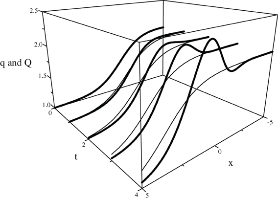
Toda soliton profiles q interpolated for all x ∈ [−5, 5] at integer time slices superimposed with their time umbral maps Q (thicker curves) for a = 1.

Thus, the umbral-mapped solutions no longer evolve just by translating the profile shape. Rather, they develop oscillations about the classical fronts that dramatically increase with time, that evince not only dispersion but also generation of harmonics, and that, strictly speaking, disqualify use of the term soliton for their description. Be that as it may, this model is referred to in some studies as integrable (8, 9).

These umbral effects on wave propagation evoke scattering and diffraction by crystals. But here the “crystal” is spacetime itself. It is tempting to speculate based on this analogy. In particular, were a well-formed wave packet to pass through a localized region of crystalline spacetime, with sufficiently large lattice spacings, the packet could undergo dramatic deformations in shape, wavelength, and frequency—far greater than and very different from what would be expected just from the dispersion of a free packet propagating through continuous space and time.

6. Concluding Remarks

We have emphasized how the umbral calculus has visibly emerged to provide an elegant correspondence framework that automatically gives solutions of ubiquitous difference equations as maps of well-known continuous functions. This correspondence systematically sidesteps the use of more traditional methods to solve these difference equations.

We have used the umbral calculus framework to provide solutions to discretized versions of several differential equations that are widespread building-blocks in many if not all areas of physics and engineering, thereby avoiding the rather unwieldy frontal assaults often engaged to solve such discrete equations directly.

We have paid special attention to the Airy, Kummer, and Whittaker equations, and illustrated several basic principles that transform their continuum solutions to umbral versions through the use of hypergeometric function maps. The continuum limits thereof are then manifest.

Finally, we have applied the solution-mapping technique to single solitons of the Sine-Gordon, Korteweg–de Vries, and Toda systems, and we have noted how their umbral counterparts—particular solutions of corresponding discretized equations—evince dispersion and other non-solitonic behavior, in general. Such corrections to the continuum result may end up revealing discrete spacetime structure in astrophysical wave propagation settings.

We expect to witness several applications of the framework discussed and illustrated here.

Conflict of Interest Statement

The authors declare that the research was conducted in the absence of any commercial or financial relationships that could be construed as a potential conflict of interest.

Acknowledgments

This work was supported in part by NSF Award PHY-1214521; and in part, the submitted manuscript has been created by UChicago Argonne, LLC, Operator of Argonne National Laboratory. Argonne, a U.S. Department of Energy Office of Science laboratory, is operated under Contract No. DE-AC02-06CH11357. The U.S. Government retains for itself, and others acting on its behalf, a paid-up nonexclusive, irrevocable worldwide license in said article to reproduce, prepare derivative works, distribute copies to the public, and perform publicly and display publicly, by or on behalf of the Government. Thomas L. Curtright was also supported in part by a University of Miami Cooper Fellowship.

Footnotes

1. ^We stress that the notation [t]ⁿ is shorthand for the product t(t − a)…(t − (n − 1)a). It is not just the nth power of [t] = t.

2. ^Again we stress that e^λ[t] is a short-hand notation, and not just the usual exponential of λ[t] = λt.

3. ^N.B. There is an infinity of “non-umbral” extensions of the E(λt, λa) solution (12): Multiplying the umbral exponential by an arbitrary periodic function g(t + a) = g(t) will pass undetected through Δ, and thus will also yield an eigenfunction of Δ. Often, such extra solutions have either a vanishing continuum limit, or else an ill-defined one.

4. ^That is, for Θ ≡ arctan(a), the spacing of the zeros, period, etc, are scaled up by a factor of $\text{tanc}(\Theta )\equiv \frac{\tan (\Theta )}{\Theta }\ge 1.$ For complete periodicity on the time lattice, one further needs return to the origin in an integral number of N steps, thus a solution of N = 2πn/arctan a. Example: For a = 1, the solutions' radius spirals out as 2^t/2, while ω = π/4, and the period is τ = 8.

5. ^Recall results from using the ratio test to determine the radius of convergence for the _pF_q (α₁, …, α_p;β₁,…,β_q;x) series:

If p < q + 1 then the ratio of coefficients tends to zero. This implies that the series converges for any finite value of x.

If p = q + 1 then the ratio of coefficients tends to one, hence the series converges for |x| < 1 and diverges for |x| > 1.

If p > q + 1 then the ratio of coefficients grows without bound. The series is then divergent or asymptotic, and is a symbolic shorthand for the solution to a differential equation.

References

1. Abramowitz M, Stegun I. Handbook of Mathematical Functions., National Bureau of Standards. AMS 55, (1964).

2. Bender C, Orszag S. Advanced Mathematical Methods for Scientists and Engineers, McGraw-Hill (1978).

3. Cholewinski F, Reneke J. Electron J Diff Eq. (2003) 2003:1–64.

4. Di Bucchianico A, Loeb D. A selected survey of umbral calculus. Electron J Combin. (1995) DS3.

5. Dimakis A, Müller-Hoissen F, Striker T. Umbral calculus, discretization, and quantum mechanics on a lattice. J Phys. (1996) A 29:6861–76.

6. Floreanini R, Vinet L. Lie symmetries of finite-difference equations. J Math Phys. (1995) 36:7024–42

7. Levi D, Negro J, del Olmo M. Discrete q-derivatives and symmetries of q-difference equations. J Phys. (2004) 37:3459–73.

8. Grammaticos B, Kosmann-Schwarzbach Y, Tamizhmani T. (eds.). Discrete Integrable Systems. In: Lect Notes Phys 644:Springer (2004). doi: 10.1007/b94662.

CrossRef Full Text

9. Grammaticos B, Ramani A, Willox R. A sine-Gordon cellular automaton and its exotic solitons. J Phys A Math Theor. (2013) 46:145204.

10. Levi D, Negro J, del Olmo M. Discrete derivatives and symmetries of difference equations. J. Phys. (2001) 34:2023–2030.

11. Levi D, Tempesta P, Winternitz P. Lorentz and galilei invariance on lattices. Phys Rev. (2004a) D69:105011.

12. Levi D, Tempesta P, Winternitz P. Umbral calculus, difference equations and the discrete Schrödinger equation. J Math Phys. (2004b) 45: 4077–4105.

13. Levi D, Winternitz P. Continuous symmetries of difference equations Schiff: Loop groups and discrete KdV equations. J Phys. (2006) A39:R1–R63.

14. López-Sendino J, Negro J, Del Olmo M, Salgado E. “Quantum mechanics and umbral calculus” J. Phys. (2008) 128:012056. doi: 10.1088/1742-6596/128/1/012056

CrossRef Full Text

15. López-Sendino J, Negro J, Del Olmo M. “Discrete coulomb potential” Phys Atom. Nuclei (2010) 73.2:384–90.

16. Rota G-C. Finite Operator Calculus, Academic Press (1975).

17. Schiff J. Loop groups and discrete KdV equations. Nonlinearity (2003) 16:257–75.

18. Smirnov Y, Turbiner A. Lie algebraic discretization of differential equations. Mod Phys Lett. (1995) A10:1795 [Erratum-ibid. A10:3139 (1995)].

19. Toda M. Theory of Nonlinear Lattices (2nd Edn.) Springer (1989).

20. Ueno K. Umbral calculus and special functions; Hypergeometric series formulas through operator calculus. Adv Math. (1988) 67:174–229; Funkcialaj Ekvacioj (1990) 33:493–518.

21. Zachos CK. Umbral deformations on discrete space-time. Int J Mod Phys. (2008) A23:2005.

Appendix A: Umbral Airy Functions

Formally, these can be obtained by expressing the Airy functions in terms of hypergeometric functions and then umbral mapping the series. The continuum problem is given by

$\begin{array}{cc}{y}^{\prime \prime }-xy=0,y\left(x\right)=C_1\mathrm{AiryAi}\left(x\right)+C_2\mathrm{AiryBi}\left(x\right)\text{},& (94)\end{array}$

where

$\begin{array}{cc}\mathrm{AiryAi}\left(x\right)=\frac{1}{3^{2/3}\Gamma \left(2/3\right)}{}_0{F}_1\left(;\frac{2}{3};\frac{1}{9}{x}^3\right)-\frac{1}{3^{1/3}\Gamma \left(1/3\right)}{}_0{F}_1\left(;\frac{4}{3};\frac{1}{9}{x}^3\right)\text{},& (95)\end{array}$

$\begin{array}{cc}\mathrm{AiryBi}\left(x\right)=\frac{1}{3^{1/6}\Gamma \left(2/3\right)}{}_0{F}_1\left(;\frac{2}{3};\frac{1}{9}{x}^3\right)+\frac{3^{1/6}z}{\Gamma \left(1/3\right)}{}_0{F}_1\left(;\frac{4}{3};\frac{1}{9}{x}^3\right)\text{}.& (96)\end{array}$

The y ↦ Y umbral images of these, solving the umbral discrete difference equation (3, 12)

$\begin{array}{cc}Y(x+2a)-2Y(x+a)+Y(x)-a^{2}xY(x+a)=0,& (97)\end{array}$

are then given by (72) for k = 3. In particular,

$\begin{array}{cc}\begin{array}{l}\text{UmAiryAi}\left(x,a\right)=\frac{1}{3^{2/3}\Gamma \left(2/3\right)}{}_3{F}_1\left(-\frac{1}{3}\frac{x}{a},\frac{1}{3}\left(1-\frac{x}{a}\right),\frac{1}{3}\left(2-\frac{x}{a}\right);\frac{2}{3};-3a^3\right)\\ -\frac{1}{3^{1/3}\Gamma \left(1/3\right)}{}_3{F}_1\left(-\frac{1}{3}\frac{x}{a},\frac{1}{3}\left(1-\frac{x}{a}\right),\frac{1}{3}\left(2-\frac{x}{a}\right);\frac{4}{3};-3a^3\right)\text{}.\end{array}& (98)\end{array}$

Since the number of “numerator parameters” in the hypergeometric function ₃F₁ exceeds the number of “denominator parameters” by 2, the series expansion is at best asymptotic. However, the series is Borel summable. In this respect, the situation is the same as for the umbral gaussian (see Appendix B).

Alternatively, as previously mentioned in the text, using the familiar integral representation of AiryAi(x), the umbral map devolves to that of an exponential. That is to say,

$\begin{array}{cc}\begin{array}{l}\mathrm{AiryAi}\left(x{T}^{-1}\right)=\frac{1}{2\pi }{\displaystyle {\int }_{-\infty }^{+\infty }\exp }\left(\frac{1}{3}i{s}^3+isx{T}^{-1}\right)ds\\ \mapsto \end{array}& (99)\end{array}$

$\begin{array}{cc}\text{UmAiryAi}\left(x,a\right)=\frac{1}{2\pi }{\displaystyle {\int }_{-\infty }^{+\infty }{e}^{\frac{1}{3}i{s}^3}}{\left(1+isa\right)}^{\frac{x}{a}}ds.& (100)\end{array}$

Just as AiryAi(x) is a real function for real x, UmAiryAi(x, a) is a real function for real x and a,

$\begin{array}{cc}\text{UmAiryAi}\left(x,a\right)=\mathrm{Re}\left(\frac{1}{\pi }{\displaystyle {\int }_0^{+\infty }{e}^{\frac{1}{3}i{s}^3}}{\left(1+isa\right)}^{\frac{x}{a}}ds\right).& (101)\end{array}$

After some hand-crafting, the final result may be expressed in terms of just three ₂F₂ generalized hypergeometric functions. To wit,

$\begin{array}{ll}\begin{array}{l}\mathrm{Re}\left(\frac{1}{\pi }{\displaystyle {\int }_0^{+\infty }{e}^{\frac{1}{3}i{s}^3}}{\left(1+isw\right)}^{-z}ds\right)=C_0\left(w,z\right)\times \hfill \\ \left(8w^2\sin \left(\pi z/3\right)C_1\left(w,z\right)H_1\left(w,z\right)-12w\left(1+2\cos \left(2\pi z/3\right)\right)C_2\left(w,z\right)H_2\left(w,z\right)+3C_3\left(w,z\right)H_3\left(w,z\right)\right),\end{array}\hfill & (102)\end{array}$

where the hypergeometric functions ₂F₂ (a, b; c, d; z) appear in the expression as

$\begin{array}{cc}{H}_1\left(w,z\right)=\Gamma \left(\frac{1}{3}z\right)\Gamma \left(\frac{1}{3}+\frac{1}{3}z\right){}_2{F}_2\left(\frac{1}{3}z,\frac{1}{3}+\frac{1}{3}z;\frac{1}{3},\frac{2}{3};\frac{1}{3w^3}\right)\text{},& (103)\end{array}$

$\begin{array}{cc}{H}_2\left(w,z\right)=\Gamma \left(\frac{1}{3}+\frac{1}{3}z\right)\Gamma \left(\frac{2}{3}+\frac{1}{3}z\right){}_2{F}_2\left(\frac{1}{3}+\frac{1}{3}z,\frac{2}{3}+\frac{1}{3}z;\frac{2}{3},\frac{4}{3};\frac{1}{3w^3}\right)\text{},& (104)\end{array}$

$\begin{array}{cc}{H}_3\left(w,z\right)=\Gamma \left(\frac{2}{3}+\frac{1}{3}z\right)\Gamma \left(1+\frac{1}{3}z\right){}_2{F}_2\left(\frac{2}{3}+\frac{1}{3}z,1+\frac{1}{3}z;\frac{4}{3},\frac{5}{3};\frac{1}{3w^3}\right)\text{},& (105)\end{array}$

and where the coefficients in (102) are

$\begin{array}{cc}{C}_0\left(w,z\right)=\frac{1}{96w^2}\frac{e^{-\left(\frac{1}{3}\ln 3+\frac{1}{2}\ln w^2\right)z}}{\left(\sin \frac{1}{3}\pi z\right)\Gamma \left(\frac{1}{3}z\right)\left(\sin \frac{1}{3}\pi \left(1+z\right)\right)\Gamma \left(\frac{1}{3}+\frac{1}{3}z\right)\left(\cos \frac{1}{6}\pi \left(2z+1\right)\right)\Gamma \left(\frac{2}{3}+\frac{1}{3}z\right)},& (106)\end{array}$

$\begin{array}{cc}{C}_1\left(w,z\right)=2\sqrt[3]{3}\cos \left(\frac{1}{6}\pi z-\frac{1}{2}z\mathrm{signum}\left(w\right)\pi \right)+\sqrt[3]{3}\cos \left(\frac{1}{2}\pi z+\frac{1}{2}z\mathrm{signum}\left(w\right)\pi \right)+3^{\frac{5}{6}}\sin \left(\frac{1}{2}\pi z+\frac{1}{2}z\mathrm{signum}\left(w\right)\pi \right)\text{},& (107)\end{array}$

$\begin{array}{cc}{C}_2\left(w,z\right)=-\cos \left(\frac{1}{6}\pi +\frac{1}{6}\pi z+\frac{1}{2}\pi z\mathrm{signum}\left(w\right)\right)+\sqrt{3}\sin \left(\frac{1}{6}\pi +\frac{1}{6}\pi z+\frac{1}{2}\pi z\mathrm{signum}\left(w\right)\right)\text{},& (108)\end{array}$

$\begin{array}{cc}\begin{array}{l}{C}_3\left(w,z\right)=3\sqrt[6]{3}\cos \left(\frac{1}{2}\pi z-\frac{1}{2}\pi z\mathrm{signum}\left(w\right)\right)-6\sqrt[6]{3}\cos \left(\frac{1}{6}\pi z+\frac{1}{2}\pi z\mathrm{signum}\left(w\right)\right)\\ +6\sqrt[6]{3}\cos \left(\frac{5}{6}\pi z+\frac{1}{2}\pi z\mathrm{signum}\left(w\right)\right)+3\times 3^{\frac{2}{3}}\sin \left(\frac{1}{2}\pi z-\frac{1}{2}\pi z\mathrm{signum}\left(w\right)\right)\\ -3\sqrt[6]{3}\cos \left(\frac{1}{2}\pi z-\frac{1}{2}\pi z\mathrm{signum}\left(w\right)\right)+2\times 3^{\frac{2}{3}}\sin \left(\frac{1}{6}\pi z+\frac{1}{2}z\pi \mathrm{signum}\left(w\right)\right)\\ +3^{\frac{2}{3}}\sin \left(\frac{1}{2}\pi z+\frac{1}{2}\pi z\mathrm{signum}\left(w\right)\right)+2\times 3^{\frac{2}{3}}\sin \left(\frac{5}{6}\pi z+\frac{1}{2}\pi z\mathrm{signum}\left(w\right)\right).\end{array}& (109)\end{array}$

While the coefficient functions C₀₋₃ are not pretty, they are comprised of elementary functions, and they are nonsingular functions of z. On the other hand, the hypergeometric functions do have singularities and discontinuities for negative z. However, the net result for UmAiryAi is reasonably well-behaved.

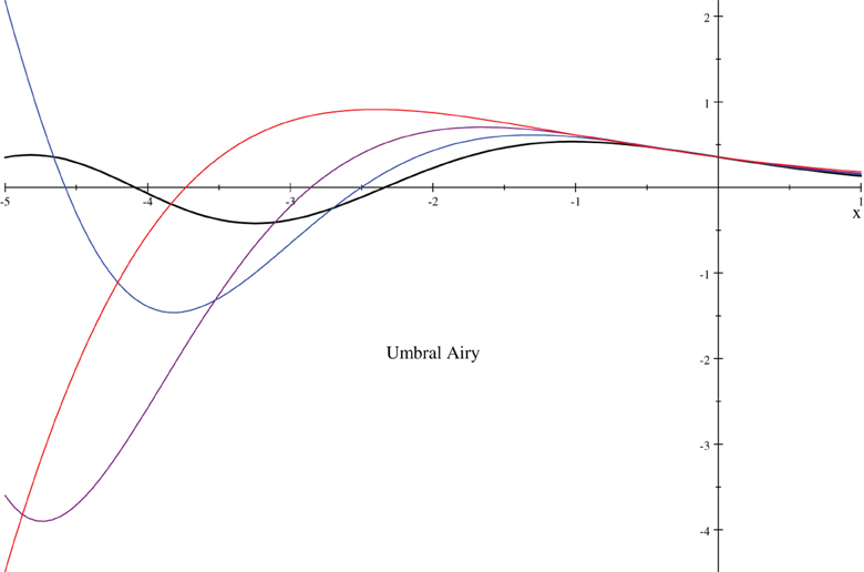
We plot UmAiryAi(x, a) for $a=0,\pm \frac{1}{4},\pm \frac{1}{2},$ and ±1.

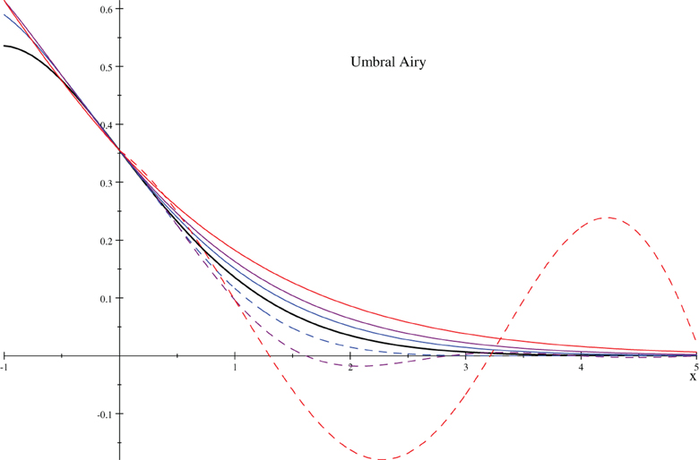
UmAiryAi(x, a) for a = ±1, ±1/2, and ±1/4 (red, blue, & green dashed/solid curves, resp.) compared to AiryAi(x) = UmAiryAi(x, 0) (black curve).

Appendix B: Umbral Gaussians

As discussed in the text, straightforward discretization of the series yields the umbral gaussian map:

$\begin{array}{cc}{e}^{-x^2}\mapsto G\left(x,a\right)={\displaystyle \sum _{n=0}^{\infty }\frac{{(-)}^n{[x]}^{2n}}{n!}}={\displaystyle \sum _{n=0}^{\infty }\frac{{(-)}^n}{n!}x(x-a)\cdots (x-\left(2n-1\right)a)}& (110)\end{array}$

$\begin{array}{cc}{=}_2{F}_0\left(-\frac{1}{2}\frac{x}{a},\frac{1}{2}\left(1-\frac{x}{a}\right);-4a^2\right).& (111)\end{array}$

(NB G(x, a) ≠ G(−x, a).) Now, it is clear that term by term the series (110) reduces back to the continuum gaussian as a → 0. Nonetheless, since the series is asymptotic and not convergent for |a| > 0, it is interesting to see how this limit is obtained from other representations of the hypergeometric function in (111), in particular from using readily available numerical routines to evaluate ₂F₀ for specific small values of a. Some examples are shown here.

G(x, 1/2ⁿ) vs. x ∈ [−3,2], for n = 1, 2, and 3, in red, blue, and green, respectively, compared to G(x, 0) = exp(−x²), in black.

Mathematica^ő code is available online to produce similar graphs, for those interested. It is amusing that Mathematica manipulates the Borel regularized sum to render the ₂F₀ in question in terms of Tricomi's confluent hypergeometric function U, as discussed above in the context of Kummer's Equation, cf. (53). Thus G can also be expressed in terms of ₁F₁s. The relevant identities are:

$\begin{array}{cc}G\left(x,a\right)={\left(2a\right)}^{\frac{x}{a}-1}U\left(\frac{1}{2}\left(1-\frac{x}{a}\right),\frac{3}{2},\frac{1}{4a^2}\right)=\sqrt{\pi }{\left(2a\right)}^{\frac{x}{a}}\left(\frac{{}_1{F}_1\left(-\frac{1}{2}\frac{x}{a};\frac{1}{2};\frac{1}{4a^2}\right)}{\Gamma \left(\frac{1}{2}\left(1-\frac{x}{a}\right)\right)}-\frac{{}_1{F}_1\left(\frac{1}{2}\left(1-\frac{x}{a}\right);\frac{3}{2};\frac{1}{4a^2}\right)}{a\Gamma \left(-\frac{1}{2}\frac{x}{a}\right)}\right).& (112)\end{array}$