Microanisotropy imaging: quantification of microscopic diffusion anisotropy and orientational order parameter by diffusion MRI with magic-angle spinning of the q-vector

Introduction

Molecular self-diffusion measured with nuclear magnetic resonance (NMR) [1, 2] can be used to non-invasively probe the microstructure of porous materials [3–5] and tissues [6]. The apparent self-diffusion coefficient, as measured in a pulsed gradient spin echo (PGSE) experiment, reflects the average diffusivity, which is a sum of contributions from different water compartments in a complex system. The diffusion is influenced by several properties of the medium, e.g., pore size and shape [7, 8], pore size distribution, pore interconnectivity [9, 10], permeability of cell membranes [11], and anisotropy [12]. The anisotropy of the tissue morphology renders the water self-diffusion anisotropic, a feature that is the basis for non-invasive mapping of muscle and nerve fiber orientations by diffusion tensor imaging (DTI) [13, 14]. DTI is commonly used to study the white matter (WM) of the brain, where the nerve fibers have a dominant direction on macroscopic length scales. Because of the limited spatial resolution in DTI, a majority of the voxels in WM contain fiber bundles with different orientations, thus making the interpretation of the DTI data ambiguous [15]. Due to the significance of accurate quantification of the level of anisotropy in the brain, techniques for detecting fiber orientation dispersion are being developed [16, 17].

The degree of the macroscopic diffusion anisotropy is often quantified by the dimensionless fractional anisotropy (FA) [12]. The FA parameter is sensitive to alterations in several tissue properties, e.g., axonal diameter, axonal packing density, and degree of myelination. Changes in these properties may be associated with normal brain development, learning, and healthy ageing, but also with disorders such as Alzheimer's disease, autism, schizophrenia, mild cognitive impairment, multiple sclerosis, amyotrophic lateral sclerosis, epilepsy, Tourette's syndrome, Parkinson's disease, and Huntington's disease [16, 18, 19]. Because fiber orientation dispersion and several other tissue properties are inherently entangled in the echo attenuation of the PGSE experiment, changes in FA are not specific to any particular tissue characteristics [16]. This fact is known to confound the use of FA as a diagnostic parameter in regions of dispersing or crossing WM fibers [17], and also detracts from the usability of FA in macroscopically isotropic tissues such as the gray matter (GM) of the nervous system [20].

Despite several experimental approaches attempting to assess the microscopic diffusion anisotropy in the nervous system [21], disentangling underlying tissue properties from the effects of orientation dispersion remains challenging and has inspired the development of analytical models extending beyond the standard DTI approach [22, 23]. For materials consisting of randomly oriented anisotropic microcrystallites, e.g., lyotropic liquid crystals, the presence of microscopic anisotropy can be inferred from the characteristic functional form of the PGSE signal attenuation [24, 25]. This approach becomes ambiguous for more complex materials where several mechanisms could give the same signal attenuation. More recently, the microscopic anisotropy is detected in double-PGSE experiments by diffusion encoding in two separate time periods [26], giving characteristic signal modulations for data obtained with collinear and orthogonal displacement encoding [27–29] or when systematically varying the angle between the directions of displacement encoding [26, 30, 31]. A double-PGSE scheme to quantify microscopic anisotropy in terms of compartment eccentricity, independent of the macroscopic anisotropy, has recently been suggested [32]. A two-dimensional correlation approach [33] gives the currently most complete separation of the underlying diffusion components, albeit at the expense of being far too time consuming for clinical use.

We have recently shown that microscopic anisotropy can be efficiently detected with an acquisition protocol including single-shot isotropic diffusion weighting (DW) using magic-angle spinning of the q-vector (q-MAS) [34]. Comparisons between the q-MAS and other single-shot DW approaches [35, 36] can be found in [37]. Here we implement a numerically optimized version of the q-MAS pulse sequence [37] on a high-performance microimaging system, limited to specimens with maximum 10 mm diameter, and on a standard whole-body clinical scanner. The efficiency of the q-MAS sequence is demonstrated using two materials with pronounced water diffusion anisotropy: lyotropic liquid crystals [24, 25, 27, 34, 38–40] and pureed asparagus [41–44]. For contrast, a yeast cells suspension is used, exhibiting two isotropic diffusion components [34, 45–47].

We introduce a new parameter, the microscopic fractional anisotropy (μFA), for quantification of the microscopic anisotropy, and suggest a method to estimate the value of μFA by analysis of a set of diffusion MRI data acquired with both isotropic and conventional DW. The new μFA and the standard FA parameters have the same dependence on the size, shape, and density of the underlying anisotropic compartments, but differ in their sensitivity to the distribution of compartment orientations in the image voxel. The information from FA and μFA can be combined to quantify the orientation dispersion. In the literature, there are previous definitions of an orientation dispersion index based on a specific model of the orientation distribution function [23, 48, 49]. We quantify orientation dispersion with the order parameter (OP), a well-established measure of the orientational order in the field of liquid crystals [50]. A wide range of experimental techniques have been used to estimate OP for liquid crystalline systems, e.g., NMR spectroscopy, fluorescence polarization, and X-ray scattering. We derive an expression that relates OP to FA and μFA. The analysis presented here allows disentangling the two contributions to FA, i.e., the microscopic anisotropy and the orientational order of the micro-domains.

Figure 1 illustrates idealized scenarios of microstructural organization and the corresponding μFA, OP, and FA parameters. For a purely isotropic system, FA and μFA are both zero regardless of compartment size polydispersity. For anisotropic systems on the other hand, μFA reflects anisotropy of the underlying microscopic structures but not their organization on the voxel level. For identical micro-domains with identical μFA values, a reduced FA is expected for increased orientation dispersion reflected by a reduced OP. Both FA and μFA are reduced in the presence of isotropic structures. Because of its insensitivity to orientation dispersion, μFA could potentially be used as a relevant biomarker in clinical applications. It can provide additional information about the microstructure in tissue where conventional anisotropy measures are confounded by the voxel-scale tissue organization, thus improving the diagnostic specificity. Further, μFA and OP may generate novel diagnostic information in tissue that appears isotropic on a macroscopic scale but has sub-voxel anisotropic components, such as that found in cortical GM [20].

FIGURE 1

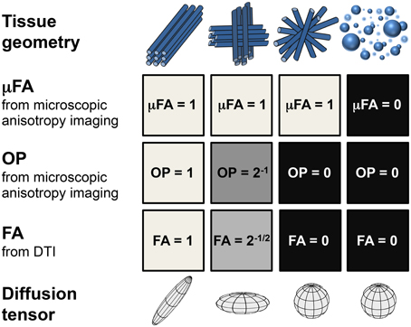
Figure 1. Idealized tissue geometries with corresponding structure parameters. Consecutive rows show values of the microscopic fractional anisotropy, μFA; orientational order parameter, OP; fractional anisotropy, FA; and diffusion tensors. Decreasing values of OP from left to right in columns 1–3 leads to a reduction of FA while μFA remains constant. For isotropic structures (column 4), both FA and μFA vanish.

Theory

Diffusion Dispersion

In complex systems like tissue, the MRI signal attenuation often reflects multiple diffusion processes, including restricted, hindered, and free diffusion. Restricted diffusion may give rise to both isotropic and anisotropic contributions. Although restricted diffusion is fundamentally a non-Gaussian process, at a low DW and at the experimental times typical for diffusion NMR/MRI, it can be characterized by the apparent diffusion coefficient, D_g, along the applied gradient direction g. For a multi-component system, the echo attenuation intensity is given by the sum over all the different contributions,

$\begin{array}{cc}{S}_g={\displaystyle \sum _i{S}_{0i}}{e}^{-b{D}_{gi}},& \left(1\right)\end{array}$

where S_0i is the relaxation weighted intensity of component i.

Equation (1) can be expressed as the Laplace transform of the probability distribution of apparent diffusivities, P(D) [25, 51, 52]. For a macroscopically anisotropic system, the distribution P(D) depends on the diffusion encoding direction, as indicated by the subscript g in Equation (1). The arithmetic average of the signal intensity over all directions, also known as the powder average, mimics a uniform orientation dispersion of anisotropic micro-domains and thus, yields P(D) independent of the orientation dispersion. Provided that P(D) is normalized to unity, the distribution is well described by the mean value,

$\begin{array}{cc}\overline{D}={\displaystyle {\int }_0^{\infty }D}P\left(D\right)dD& \left(2\right)\end{array}$

and by the central moments

$\begin{array}{cc}{\mu }_m={\displaystyle {\int }_0^{\infty }{\left(D-\overline{D}\right)}^m}P\left(D\right)dD.& \left(3\right)\end{array}$

While the mean diffusivity, D, gives the initial slope of the echo attenuation, the second central moment, μ₂, represents the initial deviation from mono-exponential attenuation, corresponding to the second term in the cumulant expansion [53] of the normalized signal intensity, E = S(b)/S₀, according to

$\begin{array}{cc}\ln E(b)=-\overline{D}b+\frac{{\mu }_2}{2}{b}^2-\mathrm{....}& \left(4\right)\end{array}$

The second central moment, μ₂, is often expressed in terms of the kurtosis coefficient K as μ₂ = D²K/3 [42]. For Gaussian diffusion in each component, as assumed in Equation (1), the value of μ₂ corresponds to the variance of apparent diffusion coefficients. For brevity, we refer to μ₂ as the variance. In the case of a two-component isotropic system, e.g., intra and extracellular diffusion in a yeast cell suspensions [34], the value of μ₂ increases with the difference between the two diffusivities and is maximized when the two contributions are represented with equal probabilities.

Microscopic Fractional Anisotropy (μFA)

The anisotropy of a medium is reflected by the diffusion tensor, D = RΛR⁻¹, where Λ is the diagonal representation of D in the principal axis system given by the eigenvalues λ₁, λ₂, and λ₃ and R is the Euler rotation matrix. In DTI, the diffusion tensor can be constructed based on measurements of signal intensity along several non-collinear gradient directions, ĝ, using the expression

$\begin{array}{cc}{S}_{\text{g}}=S_0\exp \left[-b\widehat{g}·D·{\widehat{g}}^{\text{T}}\right]\text{}.& \left(5\right)\end{array}$

The anisotropy on a voxel level is quantified in terms of FA and expressed as an invariant of the three independent diffusion tensor eigenvalue [12],

$\begin{array}{cc}\text{FA}=\sqrt{\frac{3}{2}}\sqrt{\frac{{\left({\lambda }_1-\overline{D}\right)}^2+{\left({\lambda }_2-\overline{D}\right)}^2+{\left({\lambda }_3-\overline{D}\right)}^2}{{\lambda }_1^2+{\lambda }_2^2+{\lambda }_3^2}},& \left(6\right)\end{array}$

where the mean diffusivity is given by

$\begin{array}{cc}\overline{D}=\frac{{\lambda }_1+{\lambda }_2+{\lambda }_3}{3}.& \left(7\right)\end{array}$

The diffusion tensor eigenvalues can be combined in several ways to represent different invariant measures characterizing the diffusion tensor shape. To quantify the degree to which the diffusion tensor reflects the planar geometry, we use the planar measure C_p [54],

$\begin{array}{cc}{C}_p=\frac{{\lambda }_2-{\lambda }_3}{{\lambda }_1},& \left(8\right)\end{array}$

assuming a descending order of the eigenvalues, λ₁ ≥ λ₂ ≥ λ₃.

For randomly oriented anisotropic domains represented by a single set of diffusion tensor eigenvalues, corresponding to the powder average, the variance of the observed P(D) is given by [55]

$\begin{array}{cc}{\mu }_2=\frac{4}{45}\left[{\left({\lambda }_1-{\lambda }_3\right)}^2+\left({\lambda }_2-{\lambda }_1\right)\left({\lambda }_2-{\lambda }_3\right)\right]\text{}.& \left(9\right)\end{array}$

For axially symmetric diffusion tensors, FA is given by

$\begin{array}{cc}\text{FA}=\frac{\left|D_{\left|\right|}-D_{\perp }\right|}{\sqrt{D_{\left|\right|}^2+2D_{\perp }^2}},& \left(10\right)\end{array}$

where D_|| is the axial diffusivity and D_⊥ is the radial diffusivity. For macroscopically isotropic systems, with axially symmetric anisotropic micro-domains, the signal attenuation and the corresponding P(D) can be expressed in a compact form (see Equations 34 and 35 in [34]).

The mean diffusivity and the variance are given by the axial and radial diffusivities as

$\begin{array}{cc}\begin{array}{l}\overline{D}=\frac{D_{\left|\right|}+2D_{\perp }}{3}\hfill \\ {\mu }_2=\frac{4}{45}{\left(D_{\left|\right|}-D_{\perp }\right)}^2\text{}.\hfill \end{array}& \left(11\right)\end{array}$

For a diffusion tensor with oblate shape, where D_|| < D_⊥, the upper limit of the variance is given by μ_{2 max} = D²/5, while for a prolate shape, where D_|| > D_⊥, μ_{2 max} = 4D²/5. For randomly oriented axially symmetric micro-domains, the FA in Equation (10) can be expressed in terms of D and μ₂ using the relations in Equation (11) as

$\begin{array}{cc}\text{FA}=\sqrt{\frac{3}{2}}{\left(1+\frac{2}{5}·\frac{1}{{\tilde{\mu }}_2}\right)}^{-\raisebox{1ex}{$1$}\!\left/ \!\raisebox{-1ex}{$2$}\right.},& \left(12\right)\end{array}$

where the ratio $\tilde{\mu }$₂ = μ₂/D² represents the scaled variance.

Isotropic DW can be achieved with q-MAS if the water molecules stay within an anisotropic micro-domain throughout the duration of the diffusion encoding [34]. In a system consisting of a single type of micro-domain, the variance μ₂, observed in the powder-averaged DW experiment, is a consequence of domain anisotropy and independent of orientation dispersion. In such a case, the isotropic DW yields μ^iso₂ = 0. Since the difference Δμ₂ = μ₂–μ^iso₂ is expected to vanish when all diffusion contributions are isotropic, and it is maximized for systems where the deviation from mono-exponential echo decay is purely due to microscopic anisotropy, the difference Δμ₂ can be used to quantify microscopic anisotropy. In case of macroscopically isotropic systems, or equivalently, for an isotropically averaged intensity, the mean diffusivity is expected to be identical for both isotropic and powder-averaged DW data. This can be implemented as an advantageous constraint in data analysis.

Substituting the $\tilde{\mu }$₂ in Equation (12) with its “bias-corrected” counterpart, here named the difference in scaled variance,

$\begin{array}{cc}\Delta {\tilde{\mu }}_2=\frac{{\mu }_2-{\mu }_2^{\text{iso}}}{{\overline{D}}^2}.& \left(13\right)\end{array}$

suggests a definition for the microscopic fractional anisotropy, μFA, according to

$\begin{array}{cc}\mu \text{FA}=\sqrt{\frac{3}{2}}{\left(1+\frac{2}{5}·\frac{1}{\Delta {\tilde{\mu }}_2}\right)}^{-\raisebox{1ex}{$1$}\!\left/ \!\raisebox{-1ex}{$2$}\right.}.& \left(14\right)\end{array}$

Equation (14) is the key equation to quantify microscopic anisotropy, since Δ$\tilde{\mu }$₂ is the measurable difference in curvature between powder-averaged and isotropic signal-vs.-b data, while μFA is the desired microstructural parameter. The relation between Δ$\tilde{\mu }$₂ and μFA is shown in Figure 2A.

FIGURE 2

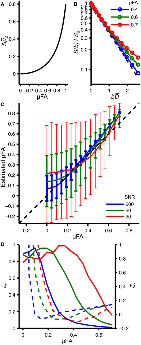
Figure 2. Random and systematic errors in estimating the microscopic fractional anisotropy. (A) Relation between microscopic fractional anisotropy (μFA) and the difference in variance, Δ$\tilde{\mu }$₂ = (μ₂ − μ^iso₂)/D², calculated with Equation (14). (B) Powder-averaged signal attenuation, S(b)/S₀, for an axially symmetric anisotropic system corresponding to different μFA values (solid lines with circles), calculated based on Equation 35 in [34] using the relations in Equations (11) and (14). The dashed line corresponds to the isotropic DW with μ^iso₂ = 0. (C) Relation between true μFA values and their estimation from fitting Equation (25) to data generated in the same way as the data shown in panel (B). Shown are the mean values (solid lines) and standard deviations (error bars) resulting from 1000 fitting iterations with synthetic noise corresponding to different SNRs [66]. (D) Relative systematic (δ_r, dashed line) and random errors (ε_r, solid lines) calculated from data shown in panel (C). In panel (B), the red, green, and blue colors correspond to different μFA values, while in panels (C,D), the colors correspond to different SNR levels.

The values of μFA are equal to the FA when diffusion is locally purely anisotropic and determined by coherently oriented axially symmetric diffusion tensors. For two-dimensional diffusion between parallel planes, μFA = FA = $\sqrt{1/2}$ and for one-dimensional diffusion within narrow tubes, μFA = FA = 1.

Order Parameter (OP)

The OP is well-established for characterization of the orientational order in liquid crystals [50]. Here we use the OP to quantify the orientation dispersion of anisotropic micro-domains. Consider a typical macroscopic voxel consisting of an ensemble of anisotropic micro-domains characterized by axially symmetric diffusion tensors with axial and radial diffusivities, D_|| and D_⊥, respectively, and varying orientation of the domain's symmetry axis d. Further, assume that the distribution of sub-voxel domain orientations is also axially symmetric around the voxel symmetry axis u, where u · d = cos θ.

The diffusivity along the voxel symmetry axis is given by the contributions from all the micro-domains with different polar angles θ. Each micro-domain contributes

$\begin{array}{cc}D\left(\theta \right)=D_{\left|\right|}{\cos }^2\theta +D_{\perp }{\sin }^2\theta .& \left(15\right)\end{array}$

Note the similarity with the expression describing the chemical shift anisotropy (see Equation 23 in [56]). The above expression can be rewritten as

$\begin{array}{cc}D\left(\theta \right)=\overline{D}+\frac{2}{3}\left(D_{\left|\right|}-D_{\perp }\right)P_2\left(\cos \theta \right),& \left(16\right)\end{array}$

where P₂(x) = (3x²–1)/2 is the second Legendre polynomial. The axial and radial diffusivities observed on a voxel level are given by the ensemble averages

$\begin{array}{cc}\begin{array}{l}\langle D_{\left|\right|}\rangle =\overline{D}+\frac{2}{3}\left(D_{\left|\right|}-D_{\perp }\right)\langle P_2\left(\cos \theta \right)\rangle \text{},\\ \langle D_{\perp }\rangle =\overline{D}+\frac{2}{3}\left(D_{\left|\right|}-D_{\perp }\right)P_2\left(\cos \frac{\pi }{2}\right)\langle P_2\left(\cos \theta \right)\rangle \\ =\overline{D}-\frac{1}{3}\left(D_{\left|\right|}-D_{\perp }\right)\langle P_2\left(\cos \theta \right)\rangle \text{}.\end{array}& \left(17\right)\end{array}$

The OP (see [50]) is defined by

$\begin{array}{cc}\text{OP}=\langle P_2\left(\cos \theta \right)\rangle \text{}.& \left(18\right)\end{array}$

As we see from Equation (17), the OP can be determined by the relation between the micro-domain diffusivities and the ensemble average diffusivities,

$\begin{array}{cc}\text{OP}=\frac{\langle D_{\left|\right|}\rangle -\langle D_{\perp }\rangle }{D_{\left|\right|}-D_{\perp }}.& \left(19\right)\end{array}$

For randomly oriented domains, the OP = 0, while for completely aligned domains, the OP = 1. The OP defined here is similar to the one calculated from motionally averaged chemical shift anisotropy or dipolar powder patterns in [50].

The definition of OP in Equation (19) is suitable for purely anisotropic systems with axial symmetry, for which μ^iso₂ = 0, and it can be determined from DW experiments performed in several non-collinear directions using multiple b-values. The ensemble average diffusivities, 〈D_||〉 and 〈D_⊥〉, are the diffusion tensor's eigenvalues, while the difference of the micro-domain diffusivities, D_|| − D_⊥, is related to the variance μ₂ in Equation (11) and can be determined by analyzing the powder-averaged signal attenuation (4). If the FA is converted into the corresponding scaled variance according to Equation (12),

$\begin{array}{cc}{\tilde{\mu }}_2^{\text{FA}}=\frac{4}{5}{\left(\frac{3}{{\text{FA}}^2}-2\right)}^{-1},& \left(20\right)\end{array}$

the OP in Equation (19) can be rewritten as $\text{OP}=\sqrt{{\tilde{\mu }}_2^{\text{FA}}/{\tilde{\mu }}_2}$. However, the FA is not only reduced due to orientation dispersion but also due to isotropic contributions, characterized by μ^iso₂ > 0. To account for the isotropic contributions in the calculation of the OP, the difference in variance should be used, suggesting the definition

$\begin{array}{cc}\text{OP}=\sqrt{\frac{{\tilde{\mu }}_2^{\text{FA}}}{\Delta {\tilde{\mu }}_2}}=\sqrt{\frac{3\mu {\text{FA}}^{-\text{2}}-2}{3{\text{FA}}^{-\text{2}}-2}}.& \left(21\right)\end{array}$

Equation (21) provides the link between the FA and μFA and allows quantifying the orientation dispersion of anisotropic structures. Since the ratio FA/μFA < 1, the OP is always in the range 0–1. The macroscopic parameter, FA, can be interpreted in terms of two underlying mechanism, i.e., the anisotropy of micro-domains, given by μFA, and the domain organization, given by the OP. Inverting Equation (21) gives

$\begin{array}{cc}\text{FA}=\text{OP}{\left[\mu {\text{FA}}^{\text{-2}}+\frac{2}{3}\left({\text{OP}}^2-1\right)\right]}^{-1/2}.& \left(22\right)\end{array}$

The above equation quantifies the relation between the anisotropy of microscopic structures and their macroscopic organization. For large FA, both the OP and the μFA need to be large, while a reduction of either OP or μFA gives reduced FA (see Figure 1).

Estimating Microscopic Fractional Anisotropy

In the case of high signal-to-noise and a well-sampled echo attenuation signal, the variance μ₂ could be estimated by regressing Equation (4) onto the isotropic and powder-averaged DW data. However, it can be shown that the convergence of the cumulant expansion is very slow in the case of randomly oriented anisotropic domains, for which the echo intensity can be expressed in a simple analytical form (see Equation 35 in [34]). The problem of analyzing the echo intensity data can instead be considered from the perspective of finding a suitable approximation to the P(D) or its first two moments, see Equations (2) and (3). A convenient functional form to approximate P(D) for complex systems with both isotropic and anisotropic components should have a simple analytical Laplace transform and it should be able to capture a wide range of diffusion distributions with only a few parameters. The gamma distribution function,

$\begin{array}{cc}P\left(D\right)=D^{\alpha -1}\frac{e^{-D/\beta }}{\Gamma \left(\alpha \right){\beta }^{\alpha }}& \left(23\right)\end{array}$

proves to be an efficient and physically plausible model for describing complex polydisperse systems such as polymer solutions [57]. The mean and the dispersion value of the gamma distribution are given by the so-called shape parameter α and the scale parameter β, where D = α · β and μ₂ = α · β², respectively. The Laplace transform of the gamma distribution takes a simple analytical form,

$\begin{array}{cc}E\left(b\right)={\left(1+b\beta \right)}^{-\alpha },& \left(24\right)\end{array}$

which can expressed as

$\begin{array}{cc}S\left(b\right)=S_0{\left(1+b\frac{{\mu }_2}{\overline{D}}\right)}^{-\frac{{\overline{D}}^2}{{\mu }_2}}& \left(25\right)\end{array}$

for data-fitting purposes.

Figure 2 summarizes the key aspects of the microscopic anisotropy analysis, which are discussed in more detail throughout the Results and Discussion section. The functional form of Equation (14) is shown in Figure 2A. The expected signal attenuation for an axially symmetric anisotropic system with varying μFA values is depicted in Figure 2B, illustrating that only rather large μFA values give rise to a detectable deviation from mono-exponential decay. The systematic and random errors of μFA estimation resulting from fitting Equation (25) to the synthetic data in Figure 2B are presented in Figures 2C,D.

Materials and Methods

Liquid Crystal/Yeast Phantom

A liquid crystalline sample was prepared by mixing the nonionic surfactant triethylene glycol monodecyl ether C₁₀E₃ (Nikko Chemical Co., Tokyo, Japan) with water containing 95 wt% D₂O (Sigma Aldrich, Steinheim, Germany) and 5 wt% H₂O (MilliQ purified) in an NMR tube with 5 mm outer diameter, giving 40 wt% surfactant concentration and 0.5 ml sample volume. A water bath was used to heat the sample to 50°C where it separates into two phases: nearly pure water and a concentrated surfactant solution with reverse micelles [58], both phases having low viscosity. After removing the tube from the water bath and exposing it to room temperature air, it was held horizontally and rotated manually about its long axis until, after approximately 2 min, the sample turned viscous. The temperature decrease leads to a phase transition into the lamellar liquid crystalline phase [58], while the rotation aligns the lamellae with respect to the inner surface of the tube [59]. The preferential orientation of the lamellae extends less than a millimeter from the glass surface, thus leaving the interior of the sample randomly oriented (see Figure 3). The sample was equilibrated at room temperature (21°C) for 24 h with the tube in the vertical direction.

FIGURE 3

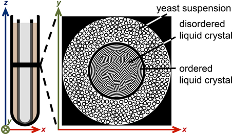
Figure 3. Illustration of the liquid crystal/yeast MRI phantom. A 5 mm NMR tube, containing 40 wt% of the surfactant C₁₀E₃ in water, is inserted into a 10 mm NMR tube with yeast cells in water. The black horizontal line in the left schematic indicates the slice of the 2D MR image. The top view of the phantom is depicted on the right. The anisotropic liquid crystal domains are mostly randomly oriented, while a narrow layer of aligned domains is formed near the tube walls.

Fresh baker's yeast was purchased at a local supermarket. A cell suspension was prepared by shaking equal volumes of the yeast with tap water in a glass tube. The suspension was allowed to sediment overnight at room temperature. The clear supernatant was discarded and 1 ml of the loosely packed cell sediment was transferred to a 10 mm NMR tube using a syringe with a 1 mm diameter needle.

The 5 mm NMR tube with the liquid crystal was inserted into the 10 mm NMR tube with the yeast sediment, creating an MRI phantom with an inner cylindrical compartment with water diffusion anisotropy and an outer cylindrical shell having a broad distribution of isotropic water diffusivities (see Figure 3). Before the MRI measurements, the sample was equilibrated for 2 h at 25°C within the magnet of the microimaging equipment.

Pureed Asparagus Phantom

Fresh asparagus (Asparagus officinalis), obtained from a local supermarket, was prepared in a plastic container that consisted of two cylindrical compartments with a diameter of approximately 8 cm. The first compartment contained water and intact asparagus stems cut to an appropriate length. The second compartment was filled with water and asparagus which was processed in a kitchen blender, resulting in a grainy puree with particle sizes well below one imaging voxel. The pureed asparagus was compressed to the bottom of the container in order to decrease the free water component in the puree. Measurements were performed at room temperature on the whole-body MR scanner.

Microimaging

The liquid crystal/yeast phantom was measured on an 11.7 T Bruker AVII-500 spectrometer equipped with a Bruker MIC-5 microimaging probe having a maximum gradient strength of 3 Tm⁻¹ and a 10 mm saddle coil radio frequency (RF) insert. Images were acquired with a TopSpin 2.1 implementation of the pulse sequence shown in Figure 4 using a single-shot RARE [60] signal read-out with 9 × 9 mm field-of-view, 64 × 32 acquisition matrix (read × phase), 10 mm slice thickness, and 65 ms duration of the echo train. The spin-echo DW block with total duration of 45 ms included two identical gradient waveforms bracketing the 180° RF pulse. Isotropic DW was achieved with the optimized q-MAS gradient modulation scheme [37]. Directional DW employed a gradient waveform giving the same time-dependence of the magnitude of the q-vector as the q-MAS modulation. The q-MAS gradient waveform was executed with duration τ = 20 ms and amplitude G = 0.405 Tm⁻¹, yielding a b-value of 5200 s/mm² according to the equation b = NCγ²G²τ³, where γ = 2.675.10⁸ radT⁻¹s⁻¹ is the ¹H gyromagnetic ratio, C = 0.0278 is a constant specific for the optimized q-MAS modulation [37], and N = 2 is the number of repetitions of the q-MAS modulation. Images were acquired for 16 b-values and 15 non-collinear gradient directions, as well as 15 repetitions of the isotropic DW, giving a total data set of 480 images. The b-values were incremented by linear steps in the gradient amplitude, while the gradient directions were chosen according to the electrostatic repulsion scheme [61, 62]. Each image was recorded as the sum of four transients with phase cycling of the RF pulses and the receiver [63]. A 1 s recycle delay gave a total experiment time of 30 min.

FIGURE 4

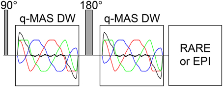
Figure 4. Schematic of the diffusion MRI pulse sequence with isotropic or directional diffusion weighting. The 90 and 180° RF pulses produce a spin echo, which is acquired with a single-shot RARE sequence at the high field spectrometer or EPI sequence at the clinical scanner. Identical DW blocks are inserted on each side of the 180° pulse. Isotropic DW is achieved with a numerically optimized q-MAS gradient modulation scheme [37] as shown with the green (G_x), blue (G_y), and red (G_z) lines. The black line indicates the directional gradient waveform that yields the same magnitude of dephasing [34] as the q-MAS modulation.

Image processing was performed with in-house Matlab code. Before Fourier transformation, the acquired data was zero-filled to 128 × 128 points [64] and multiplied with a 2D Gaussian function giving 0.2 mm × 0.2 mm image smoothing.

Whole-Body Scanner

Experiments on the pureed asparagus phantom were performed on a whole-body Philips Achieva 3 T scanner equipped with an eight-channel head coil. The gradient system delivered a maximum gradient strength of 80 mTm⁻¹ at the maximal slew rate of 100 mTm⁻¹s⁻¹. DW images were recorded with an echo planar read-out [65] using an echo time of 160 ms, half-scan factor of 0.8, SENSE factor of 2, and a slice thickness of 10 mm. The field of view was 288 × 288 mm with an acquisition matrix of 96 × 96, resulting in a spatial resolution of 3 × 3 × 10 mm³. Isotropic and directional DW were achieved during τ = 62.9 ms, before and after the 180° RF pulse, using the same waveform as in the microimagning experiment. Images were acquired for 16 b-values, between 50 and 2800 s/mm². The directional DW was performed in 15 non-collinear gradient directions spread out according to the repulsion scheme [61, 62]. The isotropic encoding was repeated 15 times for each b-value in order to generate an equal amount of acquisitions with the isotropic and directional DW. The repetition time was 2 s, resulting in acquisition times of 8:06 min for both the directional and isotropic data.

One high resolution T₂-weighted volume was acquired to visualize the different components of the phantom, and reconstructed at a spatial resolution of 0.45 × 0.45 × 8.00 mm³.

The standard scanner reconstruction software was used to convert the raw data into two series of 240 images each, which were exported to Matlab for further analysis.

Data Analysis

Maps of the eigenvalues and eigenvectors of the diffusion tensor, as well as the D and FA values were obtained by non-linear least squares fitting of directional DW data using Equation (5) with S₀, λ₁, λ₂, λ₃ and three Euler angles as adjustable parameters.

The images with directional DW (16 b-values and 15 directions) were converted to a powder-averaged series of images (16 b-values) by arithmetic averaging over the gradient directions. The multiple acquisitions of images with isotropic DW (16 b-values and 15 repetitions) were averaged to a single series (16 b-values). Equation (25) was regressed onto the isotropic and powder-averaged DW data, using S₀, D, μ₂, and μ^iso₂ as fit parameters. S₀ and D were constrained to be identical for both datasets, while μ₂ and μ^iso₂ correspond to the powder-averaged and isotropic data, respectively. The values of μ₂ and μ^iso₂ were constrained to be in the physically reasonable range from 0 to D². The standard deviations of the fit parameters were estimated by a Monte Carlo error analysis [66]. Finally, the μFA and OP indexes were calculated with Equations (14) and (21).

Results and Discussion

Phantoms, constructed to exhibit varied degree of microscopic and macroscopic anisotropy, were probed by directional and isotropic DW as well as with DTI. Results are presented and discussed in three sections; the microimaging experiments are followed by the experiments on a whole-body scanner and finally the significance of the novel microstructural measures is discussed. The microimaging section discusses the liquid crystal/yeast phantom and its micro-/macro-structural features, which are compared to the results of the μFA and DTI analysis. The difference between diffusion variance in directional and isotropic DW is thoroughly discussed in relation to the microstructural properties of the phantom. The meaning of the newly introduced parameters μFA and OP is demonstrated and the limitations of the q-MAS DW experiment and its analysis are discussed. The following section presents the results on the asparagus phantom obtained at a whole-body scanner. In the third section, the potential of μFA and OP as novel biomarkers and the key aspects of the q-MAS DW implementation in a clinical setting are considered.

Microimaging

Experimental results for the liquid crystal/yeast phantom are shown in Figure 5 as parametric images and histograms. We recapitulate that the concentric phantom is designed to have an outer compartment with a broad distribution of isotropic diffusivities and an inner compartment with microscopic diffusion anisotropy as well as varying degrees of voxel-scale anisotropy on account of the alignment of the underlying anisotropic objects with respect to the glass wall separating the two compartments (see Figure 3).

FIGURE 5

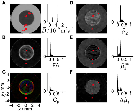
Figure 5. Parameter maps and histograms for the liquid crystal/yeast phantom. The panels show (A) mean diffusivity D, (B) fractional anisotropy FA, (C) planar index C_p, (D) scaled variance $\tilde{\mu }$₂, (E) scaled isotropic variance $\tilde{\mu }$^iso₂, and (F) the difference in scaled variance Δ$\tilde{\mu }$₂. The red crosses, numbered with roman numerals in panel (A), point out pixels for which the acquired signal is shown in detail in Figure 6. The colors in the C_p map indicate the direction of the vector corresponding to the minimum eigenvalue of the diffusion tensor (red: x, green: y, blue: z). Pixels with signal below a threshold value are shown in black in the parameter maps and excluded from the calculation of the histograms.

The map of the mean diffusivity D in Figure 5A shows clear differences between the surfactant/water mixture and the yeast suspension, with values of 0.51 and 1.5 μm²/ms, respectively, at the maxima of the narrow distributions in the histogram. A reference experiment with pure H₂O (data not shown) gives D = 2.3 μm²/ms, in good agreement with the literature value [67]. A wide range of microscopic mechanisms could cause the observed reduction of D from the value for pure H₂O: from confinement of the water in more or less impermeable micrometer-scale pores [68] to the presence of colloidal obstacles at high concentrations [69]. The values of D are by themselves not sufficient to make any detailed inferences on microstructure.

Diffusion tensor

The FA map in Figure 5B shows that the water diffusion is essentially isotropic in the yeast suspension (FA < 0.05). A closer look at the FA histogram reveals that the values for the yeast have an approximately Gaussian distribution with mean value 0.04 and standard deviation 0.02. The positive bias at low values of FA originates from the fact that any deviation from the equality λ₁ = λ₂ = λ₃ gives a positive value of FA according to Equation (6). In the surfactant/water mixture, the values of FA cover the range from 0 to 0.6, with the highest values concentrated in a 0.5 mm wide band along the outer edge of the compartment. Information about the shape and orientation of the diffusion tensor can be obtained from the planar index, C_p, color-coded with the direction of the eigenvector v₃, corresponding to the minimum eigenvalue λ₃. In Figure 5C, values of C_p above 0.7 can be observed at the rim of the interior compartment, indicating an essentially planar diffusion tensor. The radial orientation of v₃ verifies that the lamellar planes have the same orientation as the adjacent glass surface. A perfectly oriented lamellar liquid crystal, with D_|| << D_⊥, would give FA = $\sqrt{1/2}$ ≈ 0.71 and C_p = 1. The values observed experimentally, FA ≈ 0.6 and C_p = 0.7, are smaller than the ideal ones, indicating that there is a distribution of lamellar domain orientations within the voxels and/or that D_|| is not negligible in comparison to D_⊥. The values of FA and C_p are by themselves not sufficient to distinguish between the two cases. The interior of the tube with the surfactant/water mixture contains extensive regions where FA and C_p are close to zero. From the conventional DTI parameters, one could be tempted to draw the conclusion that these regions contain an isotropic phase, e.g., a sponge phase or cubic liquid crystalline phase, rather than the lamellar liquid crystalline phase that is expected from the sample composition and the equilibrium phase diagram [58].

Diffusion variance in directional and isotropic DW

Figure 5D shows the scaled variance of the distribution of apparent diffusivities P(D), $\tilde{\mu }$₂ = μ₂/D², for the powder-averaged data acquired with directional DW. We reiterate that $\tilde{\mu }$₂ is a measure of the width of the P(D) and the curvature of logS(b), and is closely related to the diffusional kurtosis [43]. Non-zero values of $\tilde{\mu }$₂ can result from diffusion anisotropy and/or the presence of more than one microscopic environment for the water. As shown in Figure 2A, diffusion anisotropy can by itself give a maximum $\tilde{\mu }$₂ value of 0.8. Both the liquid crystal and the yeast suspension display $\tilde{\mu }$₂ values being substantially different from zero. The histogram in Figure 5D features two overlapping distributions with maxima at 0.35 and 0.23 for the surfactant/water mixture and the yeast suspension, respectively. Since FA for the yeast is zero within experimental noise, it seems safe to assume that the non-zero values of $\tilde{\mu }$₂ originate from the presence of multiple microenvironments. In the case of a yeast suspension, these microenvironments correspond to the intra- and extracellular spaces [70]. Conversely, comparison between Figures 5B,D shows that, for the surfactant/water mixture, high values of $\tilde{\mu }$₂ occur for regions with both high and low values of FA, thus making the interpretation of $\tilde{\mu }$₂ in terms of either diffusion anisotropy or multiple environments highly ambiguous. The crucial information needed for discriminating between the two cases can be found in Figure 5E, displaying the scaled variance for data acquired with isotropic DW, $\tilde{\mu }$^iso₂ = μ^iso₂/D². This parameter is insensitive to diffusion anisotropy and is non-zero only if there are multiple environments with distinct isotropic diffusivities. While the surfactant/water mixture has values close to zero, the values for the yeast suspension are, within experimental noise, identical in Figures 5D,E, confirming the presence of a distribution of environments with different isotropic diffusivity. On account of the limited spatial resolution, the voxels at the border between the surfactant/water mixture and the yeast suspension contain signal from both compartments, leading to exceptionally high values of $\tilde{\mu }$^iso₂ which can be observed as a thin bright circle in Figure 5E.

As shown in Figure 5F, taking the difference Δ$\tilde{\mu }$₂ = (μ₂ − μ^iso₂)/D² isolates the effect of diffusion anisotropy. Non-zero values of Δ$\tilde{\mu }$₂ are expected when the microscopic structure is anisotropic on the length scale of the molecular displacements during the diffusion time, typically tens of micrometers. If during the diffusion encoding, molecules would have enough time to migrate between anisotropic domains with different orientations, this would affect the diffusion variance in both isotropic and directional DW. In the limit of long diffusion times, the variance observed in a directional DW vanishes [38], while in isotropic DW the variance is expected to increase due to incoherent averaging across microdomains. The dependence of the q-MAS DW on diffusion time can be viewed in analogy to the effects of the MAS in solid-state NMR spectroscopy. The broadening of P(D) in isotropic DW corresponds to the broadening of the sidebands at low frequencies of sample MAS when the rates of spinning and reorientation are similar [71]. The Δ$\tilde{\mu }$₂ values for the yeast suspension are close to zero, consistent with isotropic diffusion. Detailed inspection of the histogram in Figure 5F reveals that the yeast data can be described with an approximately Gaussian distribution with mean 0.03 and standard deviation 0.03, thus spanning both positive and negative values. The data for the surfactant/water mixture is centered at Δ$\tilde{\mu }$₂ = 0.25 and, as for the yeast, has a standard deviation of 0.03. Assuming that the true value is homogeneous in both the liquid crystal and the yeast compartments, the observed standard deviation of 0.03 can be interpreted as the precision in the estimation of Δ$\tilde{\mu }$₂ at the current experimental settings. The observation of Δ$\tilde{\mu }$₂ values well above zero for the surfactant/water mixture is a strong indication that the water resides in an anisotropic microenvironment, in agreement with the presence of a lamellar liquid crystalline phase. In contrast to FA, the values of Δ$\tilde{\mu }$₂ do not depend on the details of the orientation distribution of the anisotropic objects within the voxel, and is consequently better suited for detecting diffusion anisotropy.

Taken together, the parameters shown in Figure 5 give a rather complete description of the nature of the water environments within each voxel. Whereas the yeast suspension contains multiple water environments ($\tilde{\mu }$^iso₂ > 0) that are isotropic (Δ$\tilde{\mu }$₂ = 0), the surfactant/water mixture consists of a single type of environment ($\tilde{\mu }$^iso₂ = 0) with diffusion anisotropy on the microscopic scale (Δ$\tilde{\mu }$₂ > 0) and varying degrees of orientation coherence on the voxel scale, from random orientations (FA = 0) to preferential alignment with the lamellae following the curvature of the glass surface (FA > 0, radial orientation of v₃).

Fractional microscopic anisotropy

The information about microscopic diffusion anisotropy lies in the difference between S(b) data acquired with isotropic or powder-averaged directional DW. We believe that it is good practice to inspect the raw data to make sure that the fitted parameters are consistent with the features that can be observed visually. Figure 2B illustrates that very small deviations from a mono-exponential form of S(b) correspond to relatively large μFA values, potentially leading to erroneous conclusion when noisy data is used to estimate μFA. Data for four representative voxels can be found in Figure 6. Plotting the data as a function of bD rather than b emphasizes the deviation from mono-exponential decay and facilitates the comparison of data from voxels having different values of D [72]. The data for voxels i and ii originate from lamellar liquid crystalline phases that are coherently oriented (FA = 0.54) and randomly oriented (FA = 0.08), respectively. The mono-exponential decay of the isotropic data shows that there is a single type of water environment within the voxel, while the pronounced multi-exponential decay of the powder-averaged data proves that this environment is anisotropic. The similarity of the data for the voxels i and ii verifies that there is no influence from the voxel-scale orientation distribution of the anisotropic objects. Completely different behavior can be observed in the data from the yeast suspension in voxel iii. In this case both the isotropic and the powder-averaged data feature pronounced and identical signal attenuation, consistent with the presence of multiple isotropic water environments. Voxel iv is located at the border between the liquid crystal and yeast suspension compartments and shows signs of both multiple environments (the isotropic data) and diffusion anisotropy (pronounced multi-exponentiality for the powder-averaged data). For now, we refrain from trying to disentangle the contributions from multiple environments with varying degrees of anisotropy, but we conjecture that our approach with isotropic DW could add sufficient information to make such deconvolution feasible in a manner analogous to the separation of isotropic and anisotropic contributions to the chemical shift in solid-state NMR spectroscopy [73].

FIGURE 6

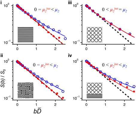
Figure 6. Normalized signal S(b)/S₀ vs. normalized diffusion weighting bD for selected pixels in Figure 5. The roman numerals of the panels correspond to the pixel labels in Figure 5A. Powder-averaged directional and isotropic data is shown with open blue and solid red circles, respectively. The solid lines indicate fits of Equation (25) to the data using S₀, D, μ₂, and μ^iso₂ as adjustable parameters. The dashed lines show the single-exponential decay S/S₀ = exp(–bD). The inserts illustrate the microstructure, with water occupying the white space between the black barriers: (i) single-orientation anisotropic, (ii) randomly oriented anisotropic domains, (iii) water inside and between spherical compartments, and (iv) mixed case with spherical compartments and anisotropic domains. The panels are labeled with the characteristic relations between μ₂ and μ^iso₂.

The parameter Δ$\tilde{\mu }$₂ is in itself an adequate measure of diffusion anisotropy. The values of Δ$\tilde{\mu }$₂ are related to the eigenvalues of the diffusion tensor through Equation (11), covering the range from 0, for isotropic diffusion, to 0.4 when D_|| < < D_⊥ and 0.8 if D_|| >> D_⊥. The FA index has been adopted as the standard measure for voxel-scale diffusion anisotropy, and it is thus desirable to convert Δ$\tilde{\mu }$₂ to a parameter that is directly comparable with FA. As described in the theory section, we define the microscopic fractional anisotropy, μFA, as the value of FA that would be observed if all the anisotropic objects had the same orientation throughout the voxel. The value of μFA can be calculated from Δ$\tilde{\mu }$₂ using Equation (14), which is also shown as a graph in Figure 2A. A comparison of FA and μFA data for the liquid crystal/yeast phantom is shown in Figure 7. Because of the highly non-linear relation between μFA and Δ$\tilde{\mu }$₂, even moderate fit errors in Δ$\tilde{\mu }$₂ get greatly amplified in the conversion to μFA when the values of Δ$\tilde{\mu }$₂ are smaller than approximately 0.1 (see Figures 2C,D). Consequently, we select the pixels for which the conversion can be reliably performed by applying a threshold value of 0.15. With this threshold, only the pixels from the liquid crystal are included in the analysis. The histograms in Figures 7A,B show that FA covers the range from 0 to 0.6 while the values of μFA are centered at 0.76 with a standard deviation of 0.03. No correlation between μFA and FA can be discerned in the scatter plot in Figure 7C, indicating that the observed spread in μFA can be attributed to the precision of the experiment rather than any true inhomogeneity of the liquid crystal sample. Even when taking into account the spread of the data, the experimental values are consistently located above the line μFA = 0.71 which is the theoretical maximum for oblate diffusion tensors. This discrepancy originates from our procedure for estimating the values of μ₂ from the experimental data using Equation (25) as a fitting function. A positive bias of μFA, visible in Figures 2C,D, arises due to the interplay between the functional form of Equation (25) and the rather extended range of b-values used for the fit. When the gamma distribution is used to approximate the diffusion dispersion due to the orientation dispersion in purely anisotropic systems, the attenuation data can be described accurately by the function in Equation (25) only for a limited range of b-values. In the case of anisotropy with axial symmetry, for which the echo attenuation can be calculated analytically (see Equation 35 in [34]) and the exact values for D and μ₂ are given by Eq. (11), the function in Eq (25) increasingly underestimates the signal intensity at bD > 1. Thus, the μ₂ value tends to be overestimated when Equation (25) is regressed onto the dataset with too high b-values resulting in an overestimation of the μFA. The bias could be reduced by limiting the range of b-values, but unfortunately at the expense of a severe loss in precision of the fitted parameters. Finding the optimal fitting function and b-values could be decisive for the success of transferring our approach to in vivo measurements. Still, we choose to postpone further investigations of this subject.

FIGURE 7

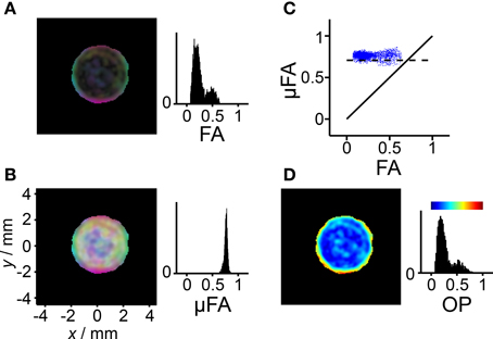
Figure 7. Diffusion anisotropy and orientation dispersion in the liquid crystal. The analysis is performed on the data from Figure 6 fulfilling the conditions D < 1μm²/ms and Δ$\tilde{\mu }$₂ > 0.15, thus excluding pixels dominated by signal from the yeast suspension. (A) Parametric map with brightness given by the fractional anisotropy (FA) and color-coding according to D_xx/λ₁ (red), D_yy/λ₁ (green), and D_zz/λ₁ (blue), where D_xx, D_yy, and D_zz are elements of the laboratory-frame diffusion tensor and λ₁ is its largest eigenvalue. (B) As in panel (A), but with brightness given by the microscopic fractional anisotropy (μFA) calculated from Δ$\tilde{\mu }$₂ in Figure 5F using Equation (14). Bright pixels with weak color saturation are observed when μFA >> FA. (C) Scatter plot showing the correlation between μFA and FA. The solid and dashed lines indicate μFA = FA and μFA = $\sqrt{1/2}$, respectively, the latter being expected for a liquid crystal with ideal lamellar geometry. (D) Parametric map and histogram of the order parameter (OP) calculated with Equation (21). The color-scale is given by the bar above the histogram. Pixels not included in the analysis are shown in black.

In the FA and μFA parameter maps in Figures 7A,B, the RGB levels are based on the three diagonal elements of the diffusion tensor in the laboratory frame of reference. The alignment of the lamellar planes at the glass surface gives rise to an intensely colored band at the outer edge of the liquid crystal compartment in both the FA and μFA maps. In stark contrast to the FA map, the brightness of the μFA map is constant on account of the nearly uniform values of μFA. Weakly colored bright pixels can be found in the interior of the compartment where there is no preferential orientation of the lamellar microcrystallites. The corresponding pixels in the FA map are nearly black because of the absence of voxel-scale anisotropy.

Order parameter

While the μFA parameter contains information about the microscopic diffusion anisotropy, the value of FA additionally includes the effect of voxel-scale alignment of the underlying anisotropic objects. Consequently, it seems logical to use the values of FA and μFA to define a parameter quantifying the orientational order or, alternatively, disorder. In the field of liquid crystals, the orientational ordering is conventionally described with an OP, defined as an ensemble average in Equation (18). In cases of lower than uniaxial symmetry, the scalar OP is generalized to an order matrix. Complete alignment of the anisotropic objects gives OP = 1, while random orientations correspond to OP = 0. Equations (19) and (21) describe how OP can be calculated from the measured diffusion tensor eigenvalues and the variances of the diffusion distribution, respectively. The eigenvalues and variances correspond to the information contained in the FA and μFA parameters, respectively. The resulting OP map for the liquid crystal is shown in Figure 7D. In line with the previous results, a highly ordered region can be found next to the glass surface, while the interior of the liquid crystal displays low order. Since the values of μFA are nearly constant, and there is a monotonous, albeit non-linear, relation between FA and OP, as described by Equations (21) and (22), the corresponding histograms in Figures 7A,D have similar shapes. The benefit of using OP, rather than some more directly calculated measure such as the ratio FA/μFA, is that it has a simple geometrical definition through Equation (18), and that it is a well-established parameter in other fields of science.

Whole-Body Scanner

Measurements of μFA were also successfully implemented on a clinical system. The highly efficient single-shot isotropic DW protocol, based on the optimized q-MAS gradient modulation [37], allows to achieve high DW even at a standard clinical scanner with significant gradient amplitude and energy constrains. It is worth noting that, although the clinical scanner was equipped with gradients capable of 80 mT/m on axis, the maximum b-value of 2800 ms/mm² for a total diffusion encoding time of 125.8 ms was mainly restricted by the power available to the gradient amplifiers. The results for the whole-body scanner imaging experiments are shown in Figure 8 as parametric maps, histograms and signal curves. The measurements were performed on a phantom consisting of one compartment that contained coherent micro domains (intact asparagus stems) and another compartment that contained small domains with high orientation dispersion (pureed asparagus).

FIGURE 8

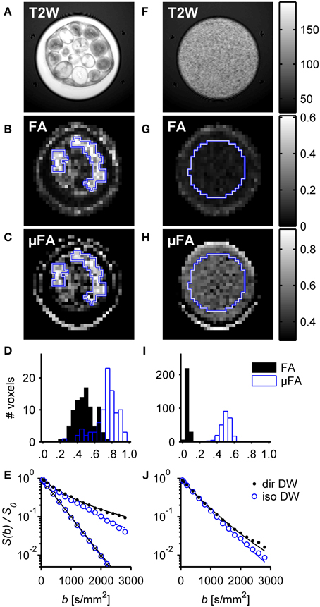
Figure 8. Results of the whole-body scanner experiment on water in intact and pureed asparagus. The left column (A–E) shows the resulting images in the intact asparagus, and the right column (F–J) shows corresponding images for the pureed asparagus. The top row shows high resolution T₂-weighted images. The second and third rows show FA and μFA maps, respectively. A high FA is only observed in the intact asparagus while μFA can be observed in both intact and pureed asparagus. The histograms show the distribution of FA and μFA in the ROIs (blue outline superimposed on FA and μFA maps). The bottom row shows normalized signal intensity vs. diffusion weighting, S(b)/S₀, for representative voxels found in the ROIs (signal from isotropic DW: empty blue circles; powder-averaged directional DW: filled black circles). The bottom left plot (E) includes the signal from a region consisting of unobstructed water measured by directional (crosses) and isotropic DW (circles). The fitted regression lines, according to Equation (25), correspond to μFA values of 0.77 and 0.47 in the intact and pureed asparagus, respectively.

The FA map for the intact asparagus phantom indicates a high degree of voxel scale anisotropy, as seen in Figure 8B. However, when the coherent geometry of the asparagus stem is distorted, as in the pureeing process, the anisotropy on the voxel scale is strongly suppressed (see Figure 8G). By contrast, the microscopic anisotropy is visible in the μFA both before and after the pureeing process, as seen in Figures 8C,H. The effects on FA and μFA were quantified using two ROIs placed in specific regions of the phantom in order to reduce the influence from the free water. The first ROI was placed over several intact asparagus stems and the second included the central parts of the asparagus puree. Notice that several stems of asparagus exhibited hyperintensity in the T₂ map, and were also found to have lower values of FA and μFA, suggesting that the micro-architecture of these stems was compromised, possibly due to mechanical damage or natural degradation. In order to avoid such damaged tissue, these stems were excluded from the ROIs. The mean parameter value in the two ROIs was FA_intact = 0.50 and FA_puree = 0.06, and μFA_intact = 0.75 and μFA_puree = 0.50, respectively. The FA value of intact asparagus is in agreement with other experiments that have employed similar diffusion times [41]. The distributions of parameter values are presented in histograms in Figures 8D,I. The histogram visualizes the high contrast between the FA and the μFA in the pureed tissue, demonstrating how the μFA is still sensitive to the anisotropic diffusion at the scale of each asparagus fragment even if the diffusion is approximately isotropic on the voxel scale. The fact that the μFA is decreased in the pureed tissue can be attributed to the loss of anisotropy in the tissue microstructure and the relatively large water component introduced in the pureeing process.

The fitted lines for the representative voxels, resulting from regression of Equation (25), are shown in Figures 8E,J. The fit parameters in the intact asparagus were D = 1.55 ± 0.05 μm²/ms, μ^iso₂ = 0.60 ± 0.12 μm⁴/ms² (μ^iso₂/D² ≈ 0.25) and μ₂ = 1.24 ± 0.18 μm⁴/ms² (μ₂/D² ≈ 0.52) resulting in a μFA value of 0.77 ± 0.03. The corresponding values in the pureed asparagus were D = 1.96 ± 0.02 μm²/ms, μ^iso₂ = 0.17 ± 0.06 μm⁴/ms² (μ^iso₂/D² ≈ 0.04) and μ₂ = 0.64 ± 0.06 μm⁴/ms² (μ₂/D² ≈ 0.17) result in a μFA value of 0.60 ± 0.02. The standard deviations were estimated by a Monte Carlo error analysis [66]. The high apparent diffusivity in the pureed asparagus tissue further supports the notion that the calculation of μFA in the pureed tissue was affected by a free water component.

Parts of the phantom with intact asparagus consist purely of unobstructed water and thus serve as a reference to validate that in these regions the isotropic and directional DW indeed yield identical signal attenuation. The signal from one such region with unobstructed water (ROI not shown), is depicted by circles and crosses in Figure 8E. The data coincide and show mono-exponential attenuation, thus verifying that the isotropic and directional experiments give the same DW for an isotropic liquid.

Significance and Implementation of Microscopic Anisotropy Biomarkers

Biophysical modeling of WM is a field that has attracted much activity lately [74], and the need to disentangle orientation dispersion from dispersion in compartment size is now obvious [23, 75, 76]. Isotropic q-MAS DW could be an important tool to help disentangle the two phenomena. We suggest that the implementation of the isotropic DW in combination with the standard high b-value directional DW may generate new valuable biomarkers, such as the μFA and OP, that would allow identifying more specific mechanisms in cases where confounders would otherwise lower the specificity of parameters such as FA. This could be particularly helpful in selective WM atrophy in crossing geometries where the removal of one fiber population would cause the FA to increase, creating an opposite effect size as compared to unidirectional geometries [17]. Unlike the FA, the μFA is not restricted to macroscopically anisotropic tissue and it is thus suited for diagnosing also macroscopically isotropic tissue such as GM, where it could detect changes in the anisotropic diffusion, a feature that is useful in the mapping of GM deterioration. The μFA could also assist in the pre-surgical planning of tumor removal by differentiating different types of tissue consistency [77].

The application of the method for in vivo quantification of microscopic anisotropy should be straight forward, but was outside the scope of this paper. Previous studies employing non-conventional diffusion encoding have produced promising results in the human brain despite the long echo times required by the signal preparation [78–80]. For accurate μFA quantification, especially in tissue close to cerebrospinal fluid, such as the cortical GM, the partial volume effect needs to be considered. Ignoring this problem is known to bias the results of conventional DTI and non-conventional diffusion MRI such as filter-exchange imaging [78, 81]. The most straightforward means of mitigating the partial volume effect would be to include an isotropic component with high-diffusivity and zero anisotropy in addition to Equation (25) for the tissue signal. Once a suitable signal model is constructed, the experiment design can be optimized to minimize the influence of noise on parameter estimates [82]. Finally, the noise-induced variance should be compared to the biological variance in μFA, to aid the design of clinical studies [83].

Conclusion

We demonstrated that the microscopic anisotropy can be quantified based on the comparison between isotropic and powder-averaged directional DW data. Proof-of-principle experiments were carried out on selected phantoms at a high-field spectrometer as well as on a standard clinical scanner. The spin-echo implementation of the optimized single-shot q-MAS DW provides efficient diffusion encoding. On the clinical scanner, q-MAS DW using echo-time of 160 ms yields b-values comparable to DKI experiments.

While adding the isotropic DW experiment to the standard DTI requires only minor additional experimental time, it adds valuable information to the powder-averaged directional DW data. In addition to FA, available from the DTI, the experiment with isotropic DW allows disentangling the contributions of microscopic anisotropy and orientation dispersion of micro-domains, which can be quantified by the herein introduced μFA and OP parameters. The μFA is not affected by the orientation dispersion of microscopic structures and it corresponds to the values of FA in the absence of orientation dispersion. Since the μFA is not sensitive to the macroscopic organization of anisotropic structures, like crossing fibers of the WM, the μFA could provide a valuable new biomarker to characterize tissue.

Author and Contributors

All the authors of this manuscript: Samo Lasič, Filip Szczepankiewicz, Stefanie Eriksson, Markus Nilsson, Daniel Topgaard, fulfill the authorship criteria according to Substantial contributions to the conception or design of the work; or the acquisition, analysis, or interpretation of data for the work; Drafting the work or revising it critically for important intellectual content; Final approval of the version to be published; and Agreement to be accountable for all aspects of the work in ensuring that questions related to the accuracy or integrity of any part of the work are appropriately investigated and resolved.

Conflict of Interest Statement

Patent applications in Sweden nr:1250453-6 and 1250452-8, applications in USA nr: 61/642 594, 61/642 589, PCT applications PCT/SE2013/050492 and PCT/SE2013/050493

Acknowledgments

The work was financially supported by the Swedish Research Council (2009–6794, 2011–4334, K2011-52x-21737-01-3), the Swedish Cancer Society (04 0421) and the National Institute of Health (NIH R01MH074794). Fruitful discussions with Carl-Fredrik Westin are gratefully acknowledged.

References

1. Callaghan PT. Translational Dynamics and Magnetic Resonance: Principles of Pulsed Gradient Spin Echo NMR. Oxford: Oxford University Press (2011).

2. Price W. NMR Studies of Translational Motion: Principles and Applications. Cambridge: Cambridge University Press (2009).

3. Hürlimann MD, Helmer KG, Latour LL, Sotak CH. Restricted diffusion in sedimentary rocks. Determination of surface-area-to-volume ratio and surface relaxivity J Magn Reson Ser A (1994) 111:169–78. doi: 10.1006/jmra.1994.1243

CrossRef Full Text

4. Topgaard D, Söderman O. Self-diffusion of nonfreezing water in porous carbohydrate polymer systems studied with nuclear magnetic resonance. Biophys J. (2002) 83:3596–606. doi: 10.1016/S0006-3495(02)75360-5

Pubmed Abstract | Pubmed Full Text | CrossRef Full Text

5. Lasič, S, Åslund I, Topgaard D. Spectral characterization of diffusion with chemical shift resolution: highly concentrated water-in-oil emulsion. J Magn Reson. (2009) 199:166–72. doi: 10.1016/j.jmr.2009.04.014

Pubmed Abstract | Pubmed Full Text | CrossRef Full Text

6. Le Bihan D. Looking into the functional architecture of the brain with diffusion MRI. Nat Rev Neurosci. (2003) 4:469–80. doi: 10.1038/nrn1119

Pubmed Abstract | Pubmed Full Text | CrossRef Full Text

7. Latour LL, Mitra PP, Kleinberg RL, Sotak CH. Time-dependent diffusion coefficient of fluids in porous media as a probe of surface-to-volume ratio. J Magn Reson Ser A (1993) 101:342–6. doi: 10.1006/jmra.1993.1056

CrossRef Full Text

8. Topgaard D, Söderman O. Experimental determination of pore shape and size using q-space NMR microscopy in the long diffusion-time limit. Magn Reson Imaging (2003) 21:69–76. doi: 10.1016/s0730-725x(02)00626-4

Pubmed Abstract | Pubmed Full Text | CrossRef Full Text

9. Latour LL, Kleinberg RL, Mitra PP, Sotak CH. Pore-size distributions and tortuosity in heterogeneous porous media. J Magn Reson Ser A (1995) 112:83–91. doi: 10.1006/jmra.1995.1012

Pubmed Abstract | Pubmed Full Text | CrossRef Full Text

10. Topgaard D, Söderman O. Diffusion of water absorbed in cellulose fibers studied with ¹H-NMR. Langmuir (2001) 17:2694–702. doi: 10.1021/la000982l

CrossRef Full Text

11. Lasič, S, Nilsson M, Lätt J, Ståhlberg F, Topgaard D. Apparent exchange rate mapping with diffusion MRI. Magn Reson Med. (2011) 66:356–65. doi: 10.1002/mrm.22782

Pubmed Abstract | Pubmed Full Text | CrossRef Full Text

12. Basser PJ, Pierpaoli C. Microstructural and physiological features of tissues elucidated by quantitative-diffusion-tensor MRI. J Magn Reson Ser B (1996) 111:209–19. doi: 10.1006/jmrb.1996.0086

Pubmed Abstract | Pubmed Full Text | CrossRef Full Text

13. Basser PJ, Mattiello J, LeBihan D. MR diffusion tensor spectroscopy and imaging. Biophys J. (1994) 66:259–67. doi: 10.1016/S0006-3495(94)80775-1

Pubmed Abstract | Pubmed Full Text | CrossRef Full Text

14. Moseley ME, Kucharczyk J, Asgari HS, Norman D. Anisotropy in diffusion-weighted MRI. Magn Reson Med. (1991) 19:321–6. doi: 10.1002/mrm.1910190222

Pubmed Abstract | Pubmed Full Text | CrossRef Full Text

15. Jeurissen B, Leemans A, Tournier J-D, Jones DK, Sijbers J. Investigating the prevalence of complex fiber configurations in white matter tissue with diffusion magnetic resonance imaging. Hum Brain Mapp. (2013) 34:2747–66. doi: 10.1002/hbm.22099

Pubmed Abstract | Pubmed Full Text | CrossRef Full Text

16. Jones DK, Knösche TR, Turner R. White matter integrity, fiber count, and other fallacies: the do's and don'ts of diffusion MRI. Neuroimage (2013) 73:239–54. doi: 10.1016/j.neuroimage.2012.06.081

Pubmed Abstract | Pubmed Full Text | CrossRef Full Text

17. Douaud G, Jbabdi S, Behrens TEJ, Menke RA, Gass A, Monsch AU, et al. DTI measures in crossing-fibre areas: increased diffusion anisotropy reveals early white matter alteration in MCI and mild Alzheimer's disease. Neuroimage (2011) 55:880–90. doi: 10.1016/j.neuroimage.2010.12.008

Pubmed Abstract | Pubmed Full Text | CrossRef Full Text

18. Sundgren PC, Dong Q, Gómez-Hassan D, Mukherji SK, Maly P, Welsh R. Diffusion tensor imaging of the brain: review of clinical applications. Neuroradiology (2004) 46:339–50. doi: 10.1007/s00234-003-1114-x

Pubmed Abstract | Pubmed Full Text | CrossRef Full Text

19. Assaf Y, Pasternak O. Diffusion tensor imaging (DTI)-based white matter mapping in brain research: a review. J Mol Neurosci. (2008) 34:51–61. doi: 10.1007/s12031-007-0029-0

Pubmed Abstract | Pubmed Full Text | CrossRef Full Text

20. McNab JA, Jbabdi S, Deoni SCL, Douaud G, Behrens TEJ, Miller KL. High resolution diffusion-weighted imaging in fixed human brain using diffusion-weighted steady state free precession. Neuroimage (2009) 46:775–85. doi: 10.1016/j.neuroimage.2009.01.008

Pubmed Abstract | Pubmed Full Text | CrossRef Full Text

21. Beaulieu C. The basis of anisotropic water diffusion in the nervous system—a technical review. NMR Biomed. (2002) 15:435–55. doi: 10.1002/nbm.782

Pubmed Abstract | Pubmed Full Text | CrossRef Full Text

22. Assaf Y, Basser PJ. Composite hindered and restricted model of diffusion (CHARMED) MR imaging of the human brain. Neuroimage (2005) 27:48–58. doi: 10.1016/j.neuroimage.2005.03.042

Pubmed Abstract | Pubmed Full Text | CrossRef Full Text

23. Zhang H, Schneider T, Wheeler-Kingshott CA, Alexander DC. NODDI: practical in vivo neurite orientation dispersion and density imaging of the human brain. Neuroimage (2012) 61:1000–16. doi: 10.1016/j.neuroimage.2012.03.072

Pubmed Abstract | Pubmed Full Text | CrossRef Full Text

24. Callaghan PT, Söderman O. Examination of the lamellar phase of Aerosol OT/water using pulsed field gradient nuclear magnetic resonance. J Phys Chem. (1983) 87:1737–44. doi: 10.1021/j100233a019

CrossRef Full Text

25. Topgaard D, Söderman O. Self-diffusion in two- and three-dimensional powders of anisotropic domains: an NMR study of the diffusion of water in cellulose and starch. J Phys Chem B (2002) 106:11887–92. doi: 10.1021/jp020130p

CrossRef Full Text

26. Mitra P. Multiple wave-vector extensions of the NMR pulsed-field-gradient spin-echo diffusion measurement. Phys Rev B (1995) 51:15074–8. doi: 10.1103/PhysRevB.51.15074

Pubmed Abstract | Pubmed Full Text | CrossRef Full Text

27. Callaghan PT, Komlosh ME. Locally anisotropic motion in a macroscopically isotropic system: displacement correlations measured using double pulsed gradient spin-echo NMR. Magn Reson Chem. (2002) 40:S15–S19. doi: 10.1002/mrc.1122

CrossRef Full Text

28. Komlosh ME, Horkay F, Freidlin RZ, Nevo U, Assaf Y, Basser PJ. Detection of microscopic anisotropy in gray matter and in a novel tissue phantom using double Pulsed Gradient Spin Echo MR. J Magn Reson. (2007) 189:38–45. doi: 10.1016/j.jmr.2007.07.003

Pubmed Abstract | Pubmed Full Text | CrossRef Full Text

29. Komlosh ME, Lizak MJ, Horkay F, Freidlin RZ, Basser PJ. Observation of microscopic diffusion anisotropy in the spinal cord using double-pulsed gradient spin echo MRI. Magn Reson Med. (2008) 59:803–9. doi: 10.1002/mrm.21528

Pubmed Abstract | Pubmed Full Text | CrossRef Full Text

30. Shemesh N, Adiri T, Cohen Y. Probing microscopic architecture of opaque heterogeneous systems using double-pulsed-field-gradient NMR. J Am Chem Soc. (2011) 133:6028–35. doi: 10.1021/ja200303h

Pubmed Abstract | Pubmed Full Text | CrossRef Full Text

31. Shemesh N, Cohen Y. Microscopic and compartment shape anisotropies in gray and white matter revealed by angular bipolar double-PFG MR. Magn Reson Med. (2011) 65:1216–27. doi: 10.1002/mrm.22738

Pubmed Abstract | Pubmed Full Text | CrossRef Full Text

32. Jespersen SN, Lundell H, Sønderby CK, Dyrby TB. Orientationally invariant metrics of apparent compartment eccentricity from double pulsed field gradient diffusion experiments. NMR Biomed. (2013) 26:1647–62. doi: 10.1002/nbm.2999

Pubmed Abstract | Pubmed Full Text | CrossRef Full Text

33. Bernin D, Topgaard D. NMR diffusion and relaxation correlation methods: new insights in heterogeneous materials. Curr Opin Colloid Interface Sci. (2013) 18:166–72. doi: 10.1016/j.cocis.2013.03.007

CrossRef Full Text

34. Eriksson S, Lasič, S, Topgaard D. Isotropic diffusion weighting in PGSE NMR by magic-angle spinning of the q-vector. J Magn Reson. (2013) 226:13–8. doi: 10.1016/j.jmr.2012.10.015

Pubmed Abstract | Pubmed Full Text | CrossRef Full Text

35. Mori S, van Zijl PC. Diffusion weighting by the trace of the diffusion tensor within a single scan. Magn Reson Med. (1995) 33:41–52. doi: 10.1002/mrm.1910330107

Pubmed Abstract | Pubmed Full Text | CrossRef Full Text

36. Wong EC, Cox RW, Song AW. Optimized isotropic diffusion weighting. Magn Reson Med. (1995) 34:139–43. doi: 10.1002/mrm.1910340202

Pubmed Abstract | Pubmed Full Text | CrossRef Full Text

37. Topgaard D. Isotropic diffusion weighting in PGSE NMR: numerical optimization of the q-MAS PGSE sequence. Micropor Mesopor Mat. (2013) 178:60–3. doi: 10.1016/j.micromeso.2013.03.009

CrossRef Full Text

38. Åslund I, Cabaleiro-Lago C, Söderman O, Topgaard D. Diffusion NMR for determining the homogeneous length-scale in lamellar phases. J Phys Chem B (2008) 112:2782–94. doi: 10.1021/jp076174l

Pubmed Abstract | Pubmed Full Text | CrossRef Full Text

39. Hubbard PL, McGrath KM, Callaghan PT. Orientational anisotropy in the polydomain lamellar phase of a lyotropic liquid crystal. Langmuir (2006) 22:3999–4003. doi: 10.1021/la052998n

Pubmed Abstract | Pubmed Full Text | CrossRef Full Text

40. Hubbard PL, McGrath KM, Callaghan PT. Evolution of a lamellar domain structure for an equilibrating lyotropic liquid crystal. J Phys Chem B (2006) 110:20781–8. doi: 10.1021/jp0601872

Pubmed Abstract | Pubmed Full Text | CrossRef Full Text

41. Lätt J, Nilsson M, Rydhög A, Wirestam R, Ståhlberg F, Brockstedt S. Effects of restricted diffusion in a biological phantom: a q-space diffusion MRI study of asparagus stems at a 3T clinical scanner. MAGMA (2007) 20:213–22. doi: 10.1007/s10334-007-0085-z

Pubmed Abstract | Pubmed Full Text | CrossRef Full Text

42. Jansen JFA, Stambuk HE, Koutcher JA, Shukla-Dave A. Non-gaussian analysis of diffusion-weighted MR imaging in head and neck squamous cell carcinoma: a feasibility study. Am J Neuroradiol. (2010) 31:741–8. doi: 10.3174/ajnr.A1919

Pubmed Abstract | Pubmed Full Text | CrossRef Full Text

43. Jensen JH, Helpern JA, Ramani A, Lu H, Kaczynski K. Diffusional kurtosis imaging: the quantification of non-gaussian water diffusion by means of magnetic resonance imaging. Magn Reson Med. (2005) 53:1432–40. doi: 10.1002/mrm.20508

Pubmed Abstract | Pubmed Full Text | CrossRef Full Text

44. Paulsen JL, Cho H, Cho G, Song Y-Q. Acceleration of multi-dimensional propagator measurements with compressed sensing. J Magn Reson. (2011) 213:166–70. doi: 10.1016/j.jmr.2011.08.025

Pubmed Abstract | Pubmed Full Text | CrossRef Full Text

45. Silva MD, Helmer KG, Lee J-H, Han SS, Springer CS, Sotak CH. Deconvolution of compartmental water diffusion coefficients in yeast-cell suspensions using combined T₁ and diffusion measurements. J Magn Reson. (2002) 156:52–63. doi: 10.1006/jmre.2002.2527

Pubmed Abstract | Pubmed Full Text | CrossRef Full Text

46. Åslund I, Topgaard D. Determination of the self-diffusion coefficient of intracellular water using PGSE NMR with variable gradient pulse length. J Magn Reson. (2009) 201:250–4. doi: 10.1016/j.jmr.2009.09.006

Pubmed Abstract | Pubmed Full Text | CrossRef Full Text

47. Åslund I, Nowacka A, Nilsson M, Topgaard D. Filter-exchange PGSE NMR determination of cell membrane permeability. J Magn Reson. (2009) 200:291–5. doi: 10.1016/j.jmr.2009.07.015

Pubmed Abstract | Pubmed Full Text | CrossRef Full Text

48. Zhang H, Hubbard PL, Parker GJM, Alexander DC. Axon diameter mapping in the presence of orientation dispersion with diffusion MRI. Neuroimage (2011) 56:1301–15. doi: 10.1016/j.neuroimage.2011.01.084

Pubmed Abstract | Pubmed Full Text | CrossRef Full Text

49. Sotiropoulos SN, Behrens TEJ, Jbabdi S. Ball and rackets: inferring fiber fanning from diffusion-weighted MRI. Neuroimage (2012) 60:1412–25. doi: 10.1016/j.neuroimage.2012.01.056

Pubmed Abstract | Pubmed Full Text | CrossRef Full Text

50. Emsley JW. (ed.). Nuclear Magnetic Resonance of Liquid Crystals. Dordrecht: D. Reidel Publishing Company (1985).

51. Ronen I, Moeller S, Ugurbil K, Kim D-S. Analysis of the distribution of diffusion coefficients in cat brain at 9.4 T using the inverse Laplace transformation. Magn Reson Imaging (2006) 24:61–8. doi: 10.1016/j.mri.2005.10.023

Pubmed Abstract | Pubmed Full Text | CrossRef Full Text

52. Johnson CS Jr. Diffusion ordered nuclear magnetic resonance spectroscopy: principles and applications. Prog Nucl Magn Reson Spectrosc. (1999) 34:203–56. doi: 10.1016/s0079-6565(99)00003-5

CrossRef Full Text

53. Frisken BJ. Revisiting the method of cumulants for the analysis of dynamic light-scattering data. Appl Opt. (2001) 40:4087. doi: 10.1364/AO.40.004087

Pubmed Abstract | Pubmed Full Text | CrossRef Full Text

54. Westin CF, Maier SE, Mamata H, Nabavi A, Jolesz FA, Kikinis R. Processing and visualization for diffusion tensor MRI. Med Image Anal. (2002) 6:93–108. doi: 10.1016/S1361-8415(02)00053-1

Pubmed Abstract | Pubmed Full Text | CrossRef Full Text

55. VanderHart DL, Gutowsky HS. Rigid-lattice NMR moments and line shapes with chemical-shift anisotropy. J Chem Phys. (1968) 49:261. doi: 10.1063/1.1669820

CrossRef Full Text

56. Bloembergen N, Rowland TJ. On the nuclear magnetic resonance in metals and alloys. Acta Metall. (1953) 1:731–46. doi: 10.1016/0001-6160(53)90033-9

CrossRef Full Text

57. Röding M, Bernin D, Jonasson J, Särkkä, A, Topgaard D, Rudemo M, et al. The gamma distribution model for pulsed-field gradient NMR studies of molecular-weight distributions of polymers. J Magn Reson. (2012) 222:105–11. doi: 10.1016/j.jmr.2012.07.005

Pubmed Abstract | Pubmed Full Text | CrossRef Full Text

58. Le TD, Olsson U, Mortensen K, Zipfel J, Richtering W. Nonionic amphiphilic bilayer structures under shear. Langmuir (2001) 17:999–1008. doi: 10.1021/la001227a

CrossRef Full Text

59. Oliviero C, Coppola L, Gianferri R, Nicotera I, Olsson U. Dynamic phase diagram and onion formation in the system C₁₀E₃/D₂O. Colloids Surface A (2003) 228:85–90. doi: 10.1016/S0927-7757(03)00356-X

CrossRef Full Text

60. Hennig J, Nauerth A, Friedburg H. RARE imaging: a fast imaging method for clinical MR. Magn Reson Med. (1986) 3:823–33. doi: 10.1002/mrm.1910030602

Pubmed Abstract | Pubmed Full Text | CrossRef Full Text

61. Bak M, Nielsen N. REPULSION, a novel approach to efficient powder averaging in solid-state NMR. J Magn Reson. (1997) 125:132–9. doi: 10.1006/jmre.1996.1087

Pubmed Abstract | Pubmed Full Text | CrossRef Full Text

62. Jones DK, Horsfield MA, Simmons A. Optimal strategies for measuring diffusion in anisotropic systems by magnetic resonance imaging. Magn Reson Med. (1999) 42:515–25. doi: 10.1002/(SICI)1522-2594(199909)42:3<515::AID-MRM14>3.0.CO;2-Q

Pubmed Abstract | Pubmed Full Text | CrossRef Full Text

63. Bodenhausen G, Freeman R, Turner DL. Suppression of artifacts in two-dimensional J spectroscopy. J Magn Reson. (1977) 27:511–4. doi: 10.1016/0022-2364(77)90016-6

CrossRef Full Text

64. Zhu X, Tomanek B, Sharp J. A pixel is an artifact: on the necessity of zero-filling in fourier imaging. Concepts Magn Reson Part A (2013) 42:32–44. doi: 10.1002/cmr.a.21256

CrossRef Full Text

65. Mansfield P. Multi-planar image formation using NMR spin echoes. J Phys C Solid State Phys. (1977) 10:L55–L58. doi: 10.1088/0022-3719/10/3/004

CrossRef Full Text

66. Alper JS, Gelb RI. Standard errors and confidence intervals in nonlinear regression: comparison of Monte Carlo and parametric statistics. J Phys Chem. (1990) 94:4747–51. doi: 10.1021/j100374a068

CrossRef Full Text

67. Price WS, Ide H, Arata Y. Self-diffusion of supercooled water to 238 K using PGSE NMR diffusion measurements. J Phys Chem A (1999) 103:448–50. doi: 10.1021/jp9839044

CrossRef Full Text

68. Stejskal EO. Use of spin echoes in a pulsed magnetic-field gradient to study anisotropic, restricted diffusion and flow. J Chem Phys. (1965) 43:3597. doi: 10.1063/1.1696526

CrossRef Full Text

69. Jönsson B, Wennerström H, Nilsson PG, Linse P. Self-diffusion of small molecules in colloidal systems. Colloid Polym Sci. (1986) 264:77–88. doi: 10.1007/BF01410310

CrossRef Full Text

70. Malmborg C, Sjöbeck M, Brockstedt S, Englund E, Söderman O, Topgaard D. Mapping the intracellular fraction of water by varying the gradient pulse length in q-space diffusion MRI. J Magn Reson. (2006) 180:280–5. doi: 10.1016/j.jmr.2006.03.005

Pubmed Abstract | Pubmed Full Text | CrossRef Full Text

71. Suwelack D, Rothwell WP, Waugh JS. Slow molecular motion detected in the NMR spectra of rotating solids. J Chem Phys. (1980) 73:2559. doi: 10.1063/1.440491

CrossRef Full Text

72. Svensson A, Topgaard D, Piculell L, Söderman O. Molecular self-diffusion in micellar and discrete cubic phases of an ionic surfactant with mixed monovalent/polymeric counterions. J Phys Chem B (2003) 107:13241–50. doi: 10.1021/jp0348225

CrossRef Full Text

73. Tycko R, Dabbagh G, Mirau PA. Determination of chemical-shift-anisotropy lineshapes in a two-dimensional magic-angle-spinning NMR experiment. J Magn Reson. (1989) 85:265–74. doi: 10.1016/0022-2364(89)90142-X

Pubmed Abstract | Pubmed Full Text | CrossRef Full Text

74. Nilsson M, van Westen D, Ståhlberg F, Sundgren PC, Lätt J. The role of tissue microstructure and water exchange in biophysical modelling of diffusion in white matter. MAGMA (2013) 26:345–70. doi: 10.1007/s10334-013-0371-x

Pubmed Abstract | Pubmed Full Text | CrossRef Full Text

75. Nilsson M, Lätt J, Ståhlberg F, van Westen D, Hagslätt H. The importance of axonal undulation in diffusion MR measurements: a Monte Carlo simulation study. NMR Biomed. (2012) 25:795–805. doi: 10.1002/nbm.1795

Pubmed Abstract | Pubmed Full Text | CrossRef Full Text

76. Ronen I, Budde M, Ercan E, Annese J, Techawiboonwong A, Webb A. Microstructural organization of axons in the human corpus callosum quantified by diffusion-weighted magnetic resonance spectroscopy of N-acetylaspartate and post-mortem histology. Brain Struct Funct. (2013) 1–13. doi: 10.1007/s00429-013-0600-0

Pubmed Abstract | Pubmed Full Text | CrossRef Full Text

77. Tropine A, Dellani PD, Glaser M, Bohl J, Plöner T, Vucurevic G, et al. Differentiation of fibroblastic meningiomas from other benign subtypes using diffusion tensor imaging. J Magn Reson Imaging (2007) 25:703–8. doi: 10.1002/jmri.20887

Pubmed Abstract | Pubmed Full Text | CrossRef Full Text

78. Nilsson M, Lätt J, van Westen D, Brockstedt S, Lasič, S, Ståhlberg F, et al. Noninvasive mapping of water diffusional exchange in the human brain using filter-exchange imaging. Magn Reson Med. (2013) 69:1572–80. doi: 10.1002/mrm.24395

Pubmed Abstract | Pubmed Full Text | CrossRef Full Text

79. Avram AV, Özarslan E, Sarlls JE, Basser PJ. In vivo detection of microscopic anisotropy using quadruple pulsed-field gradient (qPFG) diffusion MRI on a clinical scanner. Neuroimage (2013) 64:229–39. doi: 10.1016/j.neuroimage.2012.08.048

Pubmed Abstract | Pubmed Full Text | CrossRef Full Text

80. Lawrenz M, Finsterbusch J. Double-wave-vector diffusion-weighted imaging reveals microscopic diffusion anisotropy in the living human brain. Magn Reson Med. (2012) 69:1072–82. doi: 10.1002/mrm.24347

Pubmed Abstract | Pubmed Full Text | CrossRef Full Text

81. Pasternak O, Sochen N, Gur Y, Intrator N, Assaf Y. Free water elimination and mapping from diffusion MRI. Magn Reson Med. (2009) 62:717–30. doi: 10.1002/mrm.22055

Pubmed Abstract | Pubmed Full Text | CrossRef Full Text

82. Alexander DC. A general framework for experiment design in diffusion MRI and its application in measuring direct tissue-microstructure features. Magn Reson Med. (2008) 60:439–48. doi: 10.1002/mrm.21646

Pubmed Abstract | Pubmed Full Text | CrossRef Full Text

83. Szczepankiewicz F, Lätt J, Wirestam R, Leemans A, Sundgren P, van Westen D, et al. Variability in diffusion kurtosis imaging: impact on study design, statistical power and interpretation. Neuroimage (2013) 76:145–54. doi: 10.1016/j.neuroimage.2013.02.078

Pubmed Abstract | Pubmed Full Text | CrossRef Full Text