Ripening and focusing of aggregate size distributions with overall volume growth

1. Introduction

Characterizing the evolution of the number density and the size distribution of an assembly of aggregates in a fluid or solid matrix has intrigued chemists [1–3], physicists [4–7], and applied mathematicians [8–12] since it was first described by Ostwald [13]. Early successes in the theoretical modeling focused on describing the diffusive transport of material to the aggregates [14]. In many applications the volume fraction of the aggregates grows in time — either due to feeding by a chemical reaction, or because temperature or pressure changes lead to a change of the equilibrium volume fraction of the aggregates. Reiss [15] pointed out that the resulting sustained growth of the volume fraction of the aggregates can lead to focusing of the aggregate size distribution [see 16–18, for recent discussions]. Subsequent theoretical work focused on the ripening of the aggregate size distribution under thermodynamic equilibrium conditions, where to a good approximation the aggregate volume fraction is preserved [1, 4]. This dynamics involves aggregate ripening, a delicate balance of the evaporation of small aggregates, and the redistribution of their volume to achieve further growth of large aggregates. Assembly expectation values do not only change due to the evolution of the shape of the size distribution, but also by the change of its normalization, i.e., the number of aggregates. Independently, Lifshitz and Slyozov [4] and Wagner [1] derived scaling laws for the decay of the number of aggregates, and the resulting growth speed of the mean aggregate radius, and they determined the shape of the asymptotic size distribution. Modern expositions derive their results from the point of view of dynamic scaling theory [5, 8, 19].

Here, we revisit the problem of simultaneous growth and coarsening in the presence of overall volume growth. The increase of the aggregate volume fraction can be provided by different mechanisms: (i) a change of ambient temperature or pressure that drives the system deeper into a miscibility gap [20–22], (ii) evaporation of small particles denoted as sacrificial nano-particles, that are continuously added to the system [3], or (iii) a chemical reaction or external flux of material into the system (cf. the review of Sowers et al., [18]). Depending on context the aggregates may be bubbles, droplets or solid aggregates. However, in any case we consider aggregate growth for dilute systems where merging of aggregates and sedimentation play a negligible role.

We idealize aggregate growth and ripening by considering the setting of a sustained constant flux onto the aggregates [23] which gives rise to a linear growth of the aggregate volume fraction. For the phase separation of binary mixtures such a setting has been studied experimentally by Auernhammer et al. [24] and Lapp et al. [25]. The present work establishes that the net volume growth leads to a cross over to behavior that is remarkably different from the behavior assumed in dynamic scaling theory.

We present a new numerical algorithm that allows us to follow the aggregate growth for more than five orders of magnitude in the volume — i.e., we cover a factor of 65 in their average radius, 〈R〉. This large range is needed to settle in the asymptotic scaling regime where the form of the aggregate size distribution, and the exponents of the power-law growth describing the aggregate number density and the average volume can credibly be tested. To gain insight into the impact of the net aggregate growth, we explore the evolution of the size distribution for growth speeds, ξ, of the aggregate volume fraction that cover a range of three orders of magnitude.

Based on our numerical study we set up a theoretical analysis that is based on the evolution of the reduced aggregate radius, ρ = R/〈R〉. In line with Clark et al.'s [17] findings the ratio

$\begin{array}{cc}k=\frac{\langle R\rangle }{R_c}=1+\frac{\xi }{4\pi \sigma Dn}& (1)\end{array}$

of the average aggregate radius 〈R〉 and the critical radius R_c, that separates the size of aggregates that grow from those that shrink, is identified as the relevant control parameter that governs the evolution. For equilibrium systems the overall aggregate volume is preserved such that ξ = 0 and k = 1. When there is a net growth of the overall aggregate volume, the control parameter k is increased by the ratio of the growth rate ξ and the diffusive relaxation rate of supersaturation, 4π σ D n, where n is the number density of aggregates, D is the diffusion coefficient relevant for the transport of material to the aggregates, and σ is a length scale of the order of the interface width [cf. 5, 26, and Section 2.1 for details]. In Figure 1 we provide a central result of the present study, the phase portrait of the flow of ρ at a constant k, which will be derived and discussed in full detail in Section 4. Ripening at a fixed aggregate volume fraction, i.e., for ξ = 0, amounts to the control parameter k = 1. In this case R_c = 〈R〉 as pointed out by Lifshitz and Slyozov [4]. For ξ ≃ 0, ripening arises by the interplay of an unstable fixed point of the evolution for ρ = 1 which enforces evaporation of small aggregates, and the constraint of the overall conservation of volume that limits the growth of the larger aggregates [6, Chapter 7]. Beyond k = 3/2 this behavior changes qualitatively due to an exchange of stability bifurcation where the fixed point ρ = 1 becomes stable. In the following the consequences of this exchange on the asymptotic form and evolution of the aggregate size distribution are explicitly worked out, and compared to the numerical data.

FIGURE 1

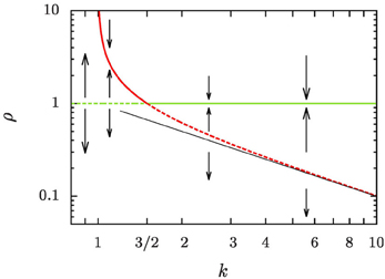
Figure 1. Phase portrait of the evolution of the reduced aggregate radius ρ = R/〈R〉. Dashed lines denote unstable fixed points, and solid lines stable ones. The green lines denotes a fixed point at ρ = 1, and the red lines the position of another fixed point, ρ₊, defined in Equation (16b). A thin straight black line has been added to show that ρ₊ rapidly approaches k⁻¹ for k ≳ 5.

The phase portrait, Figure 1, demonstrates how our discussion provides a fresh view on a number of applications that are under very active research presently: A common feature of recipes for the synthesis of nano-particles with narrow size distributions is that the focusing results from aggregate growth proceeding in the presence of sustained mass flux, that is reflected in an overall growth of the aggregate volume [3, 17, 23, 27]. In the chemical application one exploits transient focusing of the polydispersity of the larger particles in bidisperse distributions [3, 28], and in systems where there is a considerable net flux onto the aggregates [15, 27, 29, 30]. In these recipes the coarsening must be stopped once the chemical precursor reaction that provides the material condensing on the aggregates starts to cease. We argue that this is done when k drops below 3/2. Ripening would otherwise lead to a broadening of the very sharp aggregate size distributions such that eventually they approach the asymptotic Lifshitz and Slyozov [4] distribution [see the review 18].

Systems with a sustained flux onto the aggregates are also commonly encountered in the ripening and growth of bubbles in soda drinks, beer and sparkling wine [31, 32], and in many natural processes. Noticeable examples in the geo-sciences are the ripening and growth of bubbles in the depths of geysers prior to eruption [33–35], and the growth of bubbles [36], and crystallites in cooling magma [37, 38].

The paper is organized as follows: In Section 2 we derive the equations of motion for the aggregate radius, and explain how the equations are integrated numerically. For N aggregates the evolution is provided by a set of N non-linear differential equations for the respective radii. The equations are coupled because they involve moments of the size distribution. A theoretical description of the time evolution of the aggregate size distribution is obtained in three steps: In Section 3 we explore the time evolution of the relevant moments of the aggregate size distribution. This allows us in Section 4 to solve the evolution of the size of individual aggregates constrained to the time evolution of the moments. Hence, we reduce the problem of solving the set of N equations to finding the solutions of a single non-linear differential equation for N different initial conditions, which define the initial aggregate size distribution. At this point we also explore the consequences of the exchange of stability bifurcation on the evaporation of aggregates. Subsequently, in Section 5 we combine the results on the evolution of the moments and on the resulting evolution of the size of individual aggregates to obtain the evolution of the aggregate size distribution. In each step of this analysis we compare the predictions to the numerical data. The implications of our findings on different experimental systems are discussed in Section 6, and the the prime results of our study are summarized in Section 7.

2. The Assembly of Aggregate radii

In principle many different processes contribute to aggregate growth. Here, we consider the case where

• There are sufficiently few aggregates such that they grow by diffusive flux received from a mean-field background supersaturation field — analogously to Lifshitz-Slyozov-Wagner theory [5].

• The feeding rate, ξ, is sufficiently small such that it only affects the mean-field level of supersaturation. It does not interfere with the diffusion that couples the aggregates to the supersaturation [cf. 39, for a discussion of potential changes to the diffusion equation].

2.1. Evolution of the Aggregate radii and Their Volume

The supersaturation in the bulk is relaxed by diffusion onto the aggregates, causing them to grow. Following Bray [5] and Landau and Lifshitz [26], we have

$\begin{array}{cc}\dot{R}=\frac{\sigma D}{R^2}\left[\frac{R}{R_c}-1\right].& (2)\end{array}$

Here, R_c is the critical aggregate radius which depends on the supersaturation in the system, D is the pertinent concentration diffusion coefficient, and σ is a microscopic length scale which accounts for the aggregate-size dependence of the chemical potential drop that is driving the diffusive fluxes. Specifically, σ is proportional to the interfacial tension. Its full parameter dependence and characteristic values for some typical applications are provided in Section 6.

The term in square brackets in Equation (2) accounts for the effect of interfacial tension on aggregate growth. Interfacial tension penalizes small aggregates such that only aggregates with a radius larger than R_c can grow. For instance, in Lifshitz-Slyozov-Wagner theory no supersaturation is provided externally, and R_c is equal to the average radius 〈R〉. Smaller aggregates evaporate, and hence they provide the supersaturation which admits the growth of the larger aggregates.

Let us now consider the evolution of N aggregates of respective radius R_i, i = 1 … N. Their total volume is

$\begin{array}{cc}V=\frac{4\pi }{3}{\displaystyle \sum _{i=1}^N{R}_i^3}.& (3\text{a})\end{array}$

Introducing the average aggregate radius, 〈R〉 = N⁻¹ ∑_i R_i, one finds

$\begin{array}{cc}\begin{array}{l}\dot{V}=4\pi {\displaystyle \sum _i{R}_i^2}{\dot{R}}_i=4\pi \sigma D{\displaystyle \sum _i\left[\frac{R_i}{R_c}-1\right]}\\ =4\pi \sigma DN\left[\frac{\langle R\rangle }{R_c}-1\right]=4\pi \sigma DN(k-1),\end{array}& (3\text{b})\end{array}$

where we have used the definition k = 〈R〉/R_c in the last step [cf. Equation (1)]. Here and in the following the brackets 〈.〉 denote the average over the aggregate assembly,

$\langle f(R)\rangle :=\frac{1}{N}{\displaystyle \sum _{i}f}(R_i).$

In particular, 〈R〉 is the average aggregate radius, and

$\begin{array}{cc}\langle R^3\rangle =\frac{3V}{4\pi N}=3\sigma D(k-1)t.& (4)\end{array}$

There is no constant term in this equation due to an appropriate choice of the initial time t₀ such that the initial volume V₀ amounts to

$V_0=\frac{4\pi }{3}{\displaystyle \sum _i{\left(R_i(t_0)\right)}^3}=4\pi \sigma D{N}_0(k-1)t_0.$

The linear growth rate ξ of the aggregate volume fraction V/ in a system of sample volume amounts to

Together with Equation (3b) this growth implies,

such that we derive here the dependence anticipated in Equation (1).

Altogether, we find the following set of equations for the evolution of the aggregate radii, R_i,

$\begin{array}{cc}{\dot{R}}_i=\frac{\sigma D}{R_i^2}\left[k\frac{R_i}{\langle R\rangle }-1\right],i=1\dots N,& (6)\end{array}$

where k is a function of the growth rate ξ, as stated in Equation (1). The growth of the aggregate radii, R_i, is coupled in a mean-field way via the dependence of the equations on the average aggregate radius 〈R〉, and via k also explicitly on the number, N = n, of aggregates.

2.2. Numerical Implementation

The implementation of the integration scheme is detailed in the flow chart provided in Figure 2. To follow the size evolution of an assembly of aggregates, we integrate the cubes, Q_i := R³_i of their respective radii. This avoids instabilities in the numerics arising when directly integrating Equation (6) for very small aggregates. In each time step we calculate the radii, R_i, and their mean value, 〈R〉, and determine the updates of the Q_i via a predictor-corrector scheme that keeps track of the growth of the overall aggregate volume, Equation (3b). It uses a recursion to identify and remove aggregates that evaporate in a given time step. Prior to calculating 〈R〉 and using Equation (6) to determine the respective volume increments, the volume of evaporating aggregates is transferred to the volume increment to be added to the surviving aggregates.

FIGURE 2

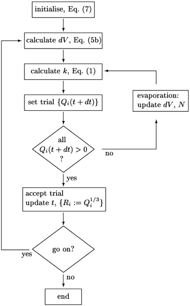
Figure 2. Schematics of the integration scheme for the size distribution {R_i}_{i = 1 … N}. The aggregate number N, the volume increments dV and the parameter k are self-consistently adjusted when small aggregates evaporate.

All numerical data in the present paper refer to an initial assembly of N₀ aggregates with a distribution that is flat in the radius between R = R_min … R_max,

$\begin{array}{cc}{R}_i=R_{\text{min}}+(R_{\text{max}}-R_{\text{min}})\frac{i-1}{N_0-1},i=1\dots N_0& (7\text{a})\end{array}$

$\begin{array}{cc}\text{with}{N}_0=1000,R_{\text{min}}=0.02,R_{\text{max}}=\mathrm{3.00.}& (7\text{b})\end{array}$

We make use of the linear growth of the overall aggregate volume, Equation (5a), to specify the elapsed time in terms of the average aggregate volume, and choose the scale for the aggregate radius such that σ D ≡ 1.

For the bookkeeping of evaporation of aggregates we observe that the increasing order of the aggregate radius with index i is preserved by the evolution. After all, Equation (6) implies that

$\begin{array}{cc}{Q}_i>Q_j\Rightarrow \frac{\text{d}}{\text{d}t}(Q_i-Q_j)=\frac{3\sigma Dk}{\langle R\rangle }(R_i-R_j)>0& (8)\end{array}$

such that the difference of the aggregate volumes grows strictly monotonically. Consequently, the evaporation of aggregates can conveniently be taken into account in our algorithm by appropriately truncating the range of the index i.

The algorithm admits adaptive step size control. After some testing we decided however to rather choose equidistant time steps on a logarithmic time axis because this saves the numerical overhead of the adaptive step size control and is convenient for the data analysis. For all data shown in this paper we took 10⁶ integration steps to increase the aggregate volume by one order of magnitude. This provides an accurate and very fast integration routine, where the simulation can span many orders of magnitude of aggregate growth.

Figure 3 shows the evolution of the cumulative aggregate size distribution (CDF), (R), for four different values of ξ that correspond to initial values of k = 5, 10, 50, and 100. The CDF provides the fraction of aggregates with a radius smaller than R. Hence, for the flat initial distribution, Equation (7), the initial CDF amounts to a function that rises linearly from zero at R_min = 0.02 to one at R_max = 3.00. This initial CDF is shown by the solid black line at the smallest values of R. To the right of this initial condition we show ten quadruples of functions displaying the respective CDFs at later times. Each set allows us to compare the shape of the CDF in a situation where the overall volume of the aggregates matches, i.e., for the same dimensionless time in our simulations. At this point we make four observations that will be further substantiated in the forthcoming discussion:

• At early times the distributions for k = 5 and 10 develop a tail toward the small aggregates, and they feature larger average aggregate sizes at late times. This is a hallmark of the evaporation of aggregates. The tail is due to aggregates that shrink and evaporate when their radius approaches zero. The larger average size is required to achieve a prescribed overall volume with a smaller number of aggregates.

• The CDFs for k = 50 and 100 look almost the same. Indeed, this holds for all k ≳ 50, where no aggregates evaporate.

• From the inspection of the numerical data one verifies that for all k > 1 the growth at late times proceeds at a fixed aggregate number. Subsequently, the difference in shape with respect to the CDFs for larger values of k does not evolve any longer.

• All distributions become more and more monodisperse.

FIGURE 3

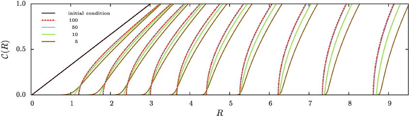
Figure 3. The four sets of curves of different color show stroboscopic snapshots of the time evolution of the cumulative size distribution function, (R), of aggregates for the same initial condition, and k = 5, 10, 50, and 100, respectively. Here and in the following we use dashed lines for the largest value of k displayed in the plot, and solid lines for all other curves. We use the same color for all data referring to a given value of k, and provide the initial conditions, Equation (7b), by a solid black line (the leftmost curve). The time increments between successive curves of the same color correspond to a time lapse resulting in an increase of the total aggregate volume by a factor of 10^1/5. Consequently, the rightmost curves of each color correspond to systems where the total aggregate volume grew by a factor of hundred. In the main text we discuss the similarities and differences between the CDFs in each of the resulting quadruplets. This allows us to pinpoint salient features of the impact of k on the time evolution of the CDFs.

The evolution of the size of individual aggregates and their evaporation is discussed in Section 4.2, and in Section 5 we address the time evolution of the CDFs. These results rest upon a priori insights into the time evolution of the moments of the aggregate size distribution that are supplied in Section 3.

3. Moments of the Aggregate Size Distribution

The set of differential Equations (6) can be decoupled when the time evolution of N and 〈R〉 can be determined a priori, i.e., without explicitly integrating the set of equations Ṙ_i. Our numerics revealed that for all k > 1 the number of aggregates N is constant at late times, and that for sufficiently large k there is no evaporation at all. In this section we therefore establish the time evolution of 〈R〉 for a constant number of aggregates, N.

3.1. Asymptotic Evolution of 〈R〉²$\frac{\text{d}}{\text{d}t}$ 〈R〉

For a constant number of particles the time derivative of the average aggregate radius

$\langle R\rangle =\frac{1}{N}{\displaystyle \sum _i{R}_i},$

based on Equation (6) is given by

$\begin{array}{cc}\frac{\text{d}}{\text{d}t}\langle R\rangle =\frac{1}{N}{\displaystyle \sum _i{\dot{R}}_i}=\frac{1}{N}{\displaystyle \sum _i\frac{\sigma D}{R_i^2}}\left[k\frac{R_i}{\langle R\rangle }-1\right]& (9\text{a})\end{array}$

$\begin{array}{cc}=\frac{\sigma D}{{\langle R\rangle }^2}\left[k\langle R^{-1}\rangle \langle R\rangle -\langle R^{-2}\rangle {\langle R\rangle }^2\right].& (9\text{b})\end{array}$

The products 〈R⁻¹〉 〈R〉 and 〈R⁻²〉 〈R〉² eventually approach one because the size distribution becomes monodisperse in the long-time limit. Hence, in this limit the characteristic aggregate volume, (4π/3) 〈R〉³, follows exactly the same growth law, Equation (4), as the average volume (4π/3) 〈R³〉,

$\begin{array}{cc}{\langle R\rangle }^2\frac{\text{d}}{\text{d}t}\langle R\rangle =\sigma D(k-1)\text{for large }t.& (10)\end{array}$

This is demonstrated in Figure 4 by showing that the ratio 〈R〉²$\frac{\text{d}}{\text{d}t}$ 〈R〉/[σD(k − 1)] settles to one after some initial transient. In order to also understand the transient decay to the growth law, Equation (10), we take a closer look at the difference of the time evolution of 〈R〉³ and 〈R³〉.

FIGURE 4

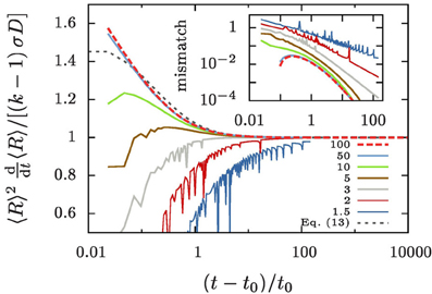
Figure 4. Evolution of 〈R〉²$\frac{\text{d}}{\text{d}t}$〈R〉 for different values of k, as indicated in the legend. The data is obtained by evaluating Equation (9b) for our numerical data. As predicted by Equation (10) it always approaches σD(k − 1) for large t. In the inset we show the mismatch of the numerical data and the improved prediction, Equation (13).

3.2. Deviation of 〈R〉³ from 〈R³〉

Equations (4, 10) state that in the long run the expectation values 〈R〉³ and 〈R³〉 acquire the same slope as functions of time. In order to gain insight into the difference of the two functions, we consider the expectation value 〈R⁴〉.

We use R = 〈R〉 + (R − 〈R〉) and the forth power of this expression to observe that

$\begin{array}{cc}\begin{array}{l}\langle R^4\rangle -{\langle R^2\rangle }^2=-\left(\langle R^2\rangle +{\langle R\rangle }^2\right)\langle {\left(R-\langle R\rangle \right)}^2\rangle \\ +6{\langle R\rangle }^2\langle {\left(R-\langle R\rangle \right)}^2\rangle \\ +4\langle R\rangle \langle {\left(R-\langle R\rangle \right)}^3\rangle +\langle {\left(R-\langle R\rangle \right)}^4\rangle \\ =4{\langle R\rangle }^2\langle {\left(R-\langle R\rangle \right)}^2\rangle [1+\frac{\langle {\left(R-\langle R\rangle \right)}^3\rangle }{\langle R\rangle \langle {\left(R-\langle R\rangle \right)}^2\rangle }\\ +\frac{\langle {\left(R-\langle R\rangle \right)}^4\rangle }{4{\langle R\rangle }^2\langle {\left(R-\langle R\rangle \right)}^2\rangle }-\frac{\langle {\left(R-\langle R\rangle \right)}^2\rangle }{4{\langle R\rangle }^2}].\end{array}& (11)\end{array}$

When approaching a monodisperse distribution the expression in square brackets rapidly approaches one, with corrections of order 〈R〉⁻². This observation provides the following insight into the leading order contributions to the difference 〈R³〉 − 〈R〉³,

$\begin{array}{l}\langle R^3\rangle =\langle {[\langle R\rangle +(R-\langle R\rangle )]}^3\rangle \\ \simeq {\langle R\rangle }^3+3\langle R\rangle \langle {\left(R-\langle R\rangle \right)}^2\rangle \\ \simeq {\langle R\rangle }^3+\frac{3}{4\langle R\rangle }\langle {(R^2-\langle R^2\rangle )}^2\rangle \end{array}$

where we used Equation (11) in the last step. Rearranging the equation yields

$\begin{array}{cc}{\langle R\rangle }^3=\langle R^3\rangle -\frac{3{\Omega }_2}{4\langle R\rangle }& (12\text{a})\end{array}$

$\begin{array}{cc}\text{with}{\Omega }_{\text{2}}\text{= }\langle {({\text{R}}^{\text{2}}-\langle {\text{R}}^{\text{2}}\rangle )}^{\text{2}}\rangle .& (12\text{b})\end{array}$

Numerical data shows that Ω₂ has a much weaker time dependence than 〈R〉⁻¹. Hence, the time derivative of Equation (12a) amounts to

$\begin{array}{cc}\begin{array}{l}{\langle R\rangle }^2\frac{\text{d}}{\text{d}t}\langle R\rangle \simeq \sigma D(k-1)+\frac{{\Omega }_2}{4{\langle R\rangle }^4}{\langle R\rangle }^2\frac{\text{d}}{\text{d}t}\langle R\rangle \\ \iff {\langle R\rangle }^2\frac{\text{d}}{\text{d}t}\langle R\rangle =\sigma D(k-1){\left(1-\frac{{\Omega }_2}{4{\langle R\rangle }^4}\right)}^{-1}.\end{array}& (13\text{a})\end{array}$

The dotted gray line in Figure 4 shows the resulting prediction when one assumes that Ω₂ never noticeably deviates from its initial value

$\begin{array}{cc}{\Omega }_2=\frac{1}{5}\frac{R_{\text{max}}^5-R_{\text{min}}^5}{R_{\text{max}}-R_{\text{min}}}-{\left(\frac{1}{3}\frac{R_{\text{max}}^3-R_{\text{min}}^3}{R_{\text{max}}-R_{\text{min}}}\right)}^2& (13\text{b})\end{array}$

determined for the initial aggregate size distribution, Equation (7b). For the specified values R_max = 3 and R_min = 0.02 it takes the value Ω₂ ≃ 7.19. The inset of Figure 4 shows the difference between this prediction and the numerical data. The strong fluctuation in the data for k ≲ 5 are due to singularities in the evolution arising when an aggregate reaches zero radius. They reflect the evaporation of aggregates, and we will not apply Equation (13) in that case since it was derived based on the assumption of no evaporation. On the other hand, for k ≳ 5 and t − t₀ ≳ t₀, i.e., once the overall aggregate volume has doubled, Equation (13) provides an accurate description of the evolution.

3.3. The Variance of the Distribution

Equations (11, 12b) provide the variance of the aggregate size distribution

$\begin{array}{cc}\langle {\left(R-\langle R\rangle \right)}^2\rangle \simeq \frac{{\Omega }_2}{4{\langle R\rangle }^2}.& (14)\end{array}$

Remarkably, the standard deviation decays like 〈R〉⁻¹. Based on the approximation that the aggregate size distribution amounts to a Gaussian at all times this result has previously been obtained by Clark et al. [17]. However, in contrast to Equation (14) these authors predicted a slightly different decay that scales like 〈R〉^{−2+2/(k−1)}. In Section 5.2 we will show that this discrepancy arises from a very slight time dependence of Ω₂: it increases like 〈R〉^2/(k−1). For large k this correction is negligible such that it is not captured by the present analysis.

The central results of this section are Equations (10, 13a). They express that one can accurately integrate the average radius 〈R〉 without need to refer to the evolution of the individual aggregates: the average 〈R〉 need not be calculated self-consistently as an average over the aggregates, but it has its own evolution equation, Equation (13a). The solution of this equation explicitly solves the global constraint that couples the set of Equations (6). Hence, the N dimensional system of non-linear coupled Equations (6) for the aggregate radii R_i is reduced to N identical one-dimensional differential equations that only differ by their initial conditions. Henceforth, we concentrate on this equation and suppress the index i.

4. The Reduced Aggregate Radius

The evolution of the decoupled set of Equations (6) is most conveniently studied based on the reduced aggregate radius ρ = R/〈R〉 that accounts for the trivial drift of the aggregate size due to the overall volume growth.

4.1. Equation of Motion

Using Equation (6) the time derivative of ρ can be written as

$\begin{array}{cc}\begin{array}{l}\dot{\rho }=\frac{d}{dt}\frac{R}{\langle R\rangle }=\frac{\dot{R}}{\langle R\rangle }-\rho \frac{\frac{\text{d}}{\text{d}t}\langle R\rangle }{\langle R\rangle }\\ =\frac{\sigma D}{\langle R\rangle R^2}\left[k\rho -1\right]-\rho \frac{\frac{\text{d}}{\text{d}t}\langle R\rangle }{\langle R\rangle }\\ =-\frac{\sigma D}{{\langle R\rangle }^3}{\rho }^{-2}\left[\frac{{\langle R\rangle }^2\frac{\text{d}}{\text{d}t}\langle R\rangle }{\sigma D}{\rho }^3-k\rho +1\right].\end{array}& (15)\end{array}$

According to Equation (10) (or Figure 4) the factor 〈R〉²$\frac{\text{d}}{\text{d}t}$〈R〉/(σD) approaches k − 1 after a short initial transient. Consequently,

$\begin{array}{cc}\begin{array}{l}\dot{\rho }\simeq -\frac{\sigma D}{{\langle R\rangle }^3}\frac{(k-1){\rho }^3-k\rho +1}{{\rho }^2}\\ =-\frac{\sigma D(k-1)}{{\langle R\rangle }^3}\frac{\left(\rho -1\right)\left(\rho -{\rho }_{-}\right)\left(\rho -{\rho }_{+}\right)}{{\rho }^2}\end{array}& (16\text{a})\end{array}$

with

$\begin{array}{cc}{\rho }_{\pm }(k)=-\frac{1}{2}\pm \frac{1}{2}\sqrt{\frac{k+3}{k-1}}.& (16\text{b})\end{array}$

The right-hand side of Equation (16a) involves a cubic polynomial in ρ (Figure 5). For all k > 1 it gives rise to three fixed points of the reduced radius: the average aggregate radius ρ = 1, a non-trivial radius ρ₊, and an unphysical fixed point ρ₋ at negative values of ρ. Discussing their positions and stability for different values of k, Figure 1, provides detailed insight into the dynamics.

k = 1: We recover classical Ostwald ripening. The radius ρ₊ diverges, and the constraint on the overall aggregate volume gives rise to an asymptotic aggregate size distribution where the largest aggregates are of radius ρ_max = 3/2.

1 < k < 3/2: Equation (16a) has an unstable fixed point at ρ = 1, i.e., for R = 〈R〉. Aggregates that are smaller than the average radius shrink and they evaporate eventually when they reach the radius ρ = 0. Aggregates larger than ρ₊ shrink, too, until they reach the stable aggregate radius ρ₊. On the other hand, aggregates in the range of 1 < ρ < ρ₊ grow at the expense of the shrinking ones, also striving to reach the aggregate radius ρ₊. When all aggregates are smaller than ρ₊ and ρ₊ ≫ 3/2 we expect a similar dynamic scaling theory to be applicable as the Lifshitz-Slyozov description of Ostwald ripening for k = 1 [see 6, for some pioneering work discussing this situation]. In the following sections we concentrate on the case k > 3/2.

k = 3/2: The fixed points ρ = 1 and ρ₊ cross, and they exchange their stability. Beyond this value aggregate evaporation ceases when all remaining aggregates have a size ρ > ρ₊.

k > 3/2: Equation (16a) has a stable fixed point for ρ = 1, and an unstable fixed point at ρ₊ which rapidly approaches k⁻¹ for k ≳ 5. After a brief initial transient no aggregates evaporate any longer, and the distribution becomes strongly peaked around the average aggregate radius 〈R〉. This is indeed what we have observed in Figure 3.

FIGURE 5

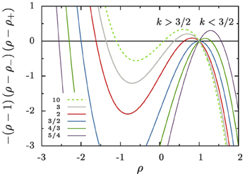
Figure 5. The cubic polynomial in the numerator of Equation (16a). For all k > 1 its three roots give rise to three fixed points of the reduced radius, ρ, that are located at ρ = 1 and ρ = ρ_±. For k = 3/2 there is a bifurcation where the roots ρ = 1 and ρ₊ change stability.

4.2. Evaporation of Aggregates

Aggregates that are smaller than ρ₊ 〈R〉 shrink and evaporate when they reach zero size. For large values of k and reasonably smooth initial aggregate densities this can only be a small fraction of aggregates. Consequently, n does not change much when these aggregates disappear. To support this view we show in Figure 6 that to an excellent approximation the number of aggregates bound to evaporate amounts to the number of aggregates in the initial distribution that lie below ρ₊.

FIGURE 6

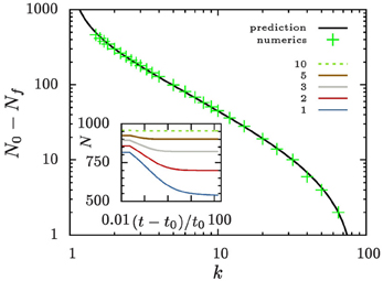
Figure 6. Evolution of the aggregate number. The inset shows the time evolution of the number of aggregates for different values of k. All systems are initialized with N0 = 1000 aggregates with a size distribution as outlined in Equation (7). Eventually, they reach a constant aggregate number, Nf. The main panel compares the number of evaporated aggregates N0 − Nf to the prediction that it should amount to ∫ρ+0 n(𝜚, t = t0) d𝜚.

The fate of a general initial distribution for an initial value of k in the range 1 < k ≤ 3/2 can be discussed based on Figure 1. For 1 < k ≤ 3/2 the aggregates with a radius smaller than average shrink, and eventually they evaporate. While doing so the number density, n, decreases. According to Equation (1) this results in an increase of k. This growth of k continues until all aggregates have a size ρ > ρ₊, i.e., their size lies above the the red line in Figure 1. At that time k takes a value k ≳ 3/2, and in the subsequent long-time limit, k is a constant of motion.

For the initial conditions specified by Equation (7) no aggregates should evaporate for R_min/〈R〉 > ρ₊ (k_c) ≃ k⁻¹_c, i.e., for k_c > 75. In practice, the numerical simulations show that k_c is slightly smaller. Systems where k > 64, i.e., ξ ≳ 250 πσ D n, evolve at a constant number density, n, of aggregates, and hence at a constant value of k. When dealing with numerical data we always indicate the initial value of k, and self-consistently take into account its change in the plots. Our focus of attention will be the asymptotics of the shape of the aggregate size distribution.

4.3. Evolution of the Reduced Aggregate Radius

For all k ≳ 3/2 and sufficiently late times the evolution of the reduced aggregate radius, ρ, can be determined explicitly by integrating Equation (15). Introducing the function

$\begin{array}{cc}a={\langle R\rangle }^3/\left[3\sigma D(k-1)\right]& (17)\end{array}$

and focusing on values ρ ≃ 1 we write

$\begin{array}{cc}\begin{array}{l}3(k-1)a{\rho }^2\dot{\rho }=-(k-1)\dot{a}{\rho }^3+(k-1)\rho +(\rho -1)\\ \simeq -(k-1)\rho \left[\dot{a}{\rho }^2-1\right]\end{array}& (18\text{a})\end{array}$

$\begin{array}{cc}\iff \frac{2}{3}{a}^{-1/3}=\frac{\text{d}}{\text{d}t}\left(a^{2/3}{\rho }^2\right).& (18\text{b})\end{array}$

This equation allows us to evaluate the derivative

$\begin{array}{cc}\begin{array}{l}\frac{\text{d}}{\text{d}t}{R}^2={\left[3\sigma D(k-1)\right]}^{2/3}\frac{\text{d}}{\text{d}t}\left(a^{2/3}{\rho }^2\right)\\ =\frac{2\sigma D(k-1)}{\langle R\rangle }\end{array}& (19\text{a})\end{array}$

which agrees with the time derivative of 〈R²〉 up to a tiny correction

$\begin{array}{cc}\begin{array}{l}\frac{\text{d}}{\text{d}t}\langle R^2\rangle =\langle 2R\dot{R}\rangle \\ =\frac{2\sigma D(k-1)}{\langle R\rangle }\left[1+\frac{1-\langle R\rangle \langle R^{-1}\rangle }{k-1}\right].\end{array}& (19\text{b})\end{array}$

Altogether, Equations (19a,b) imply that

$\begin{array}{cc}\frac{\text{d}}{\text{d}t}\left(R^2-\langle R^2\rangle \right)=0.& (20)\end{array}$

After all, there can be no merely time-dependent function appearing on the right-hand side of this equation because the expectation value 〈R² − 〈R²〉〉 must vanish at any time.

The result, Equation (20), states that at late times aggregates always grow in such a way that the difference, R² − 〈R〉², is preserved. This has immediate implications on the aggregate size distribution which will be discussed in the next section.

5. Evolution of the Aggregate Size Distribution

According to Equation (8) the order of the aggregate radii is preserved by the dynamics: when aggregate i is smaller than aggregate j initially, this holds also at all later times. Based on this observation and the explicit integration of the evolution equation of the aggregate radius, Equation (20), one can derive the aggregate size distribution. This is most easily done based on the cumulative aggregate size distribution function (CDF).

5.1. Initial Distribution, and its Evolution Based on Equation (20)

For convenience of the discussion of the asymptotic shape of the CDF, we immediately remove the aggregates from the initial distribution that will evaporate. According to the arguments underpinned by Figure 6 this amounts to the aggregates smaller than R_c = 〈R₀〉 ρ₊ (k), where 〈R₀〉 = (R_max + R_min)/2 = 1.51 is the average radius with respect to the initial aggregate size distribution (7b). When no aggregates evaporate we set R_c = R_min. With this adoption, the CDF characterizing the initial distribution, (R₀), takes the form

To avoid the involved notation required to explicitly distinguish the different branches of the function, we henceforth only specify its non-trivial branch, and keep in mind that the function should be set to zero when the expression drops below zero, and set to one when it rises beyond one.

In order to apply Equation (20) it is convenient to rewrite Equation (21) as a function of

$\begin{array}{cc}x=R^2-\langle R^2\rangle \stackrel{!}{=}{R}_0^2-\langle R_0^2\rangle .& (22)\end{array}$

In that case the non-trivial branch of the CDF takes the form of a square-root dependence

The initial condition (x) of the CDF, provided as a function of x, is shown by solid black lines in Figure 7(inset). To determine the time dependence of the CDF we note that according to Equation (22) the value of x is preserved during the evolution. Consequently, the CDF should not change in time when it is plotted as a function of x. To test this assertion the insets of Figure 7 show the initial conditions together with the CDF at later times, that are shown in colors matching those used in Figure 3. Except for the change of the variable, x rather than R, the CDFs shown in Figures 3, 7 (inset) differ only by a different choice of the time increments. A larger factor of overall volume growth has been chosen in Figure 7 in order to display distributions where the average radius grows to 〈R〉 ≃ 100 rather than only till 9.

FIGURE 7

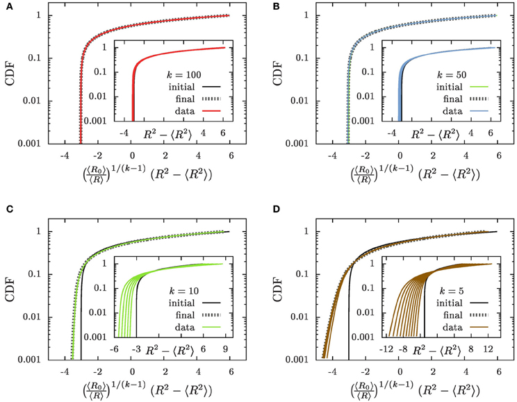
Figure 7. The CDFs (A) k = 100, (B) k = 50, (C) k = 10, and (D) k = 5. The insets show the CDFs as a function of x = R² − 〈R²〉 as suggested in Equations (22, 23), and the main panels the dependence on $\tilde{x}$ which has been defined in Equation (30). The initial conditions are provided by solid black lines labeled by the tag “initial,” and thin lines with colors matching those in Figure 3 (“data”) show the numerical results for a progression of time on a logarithmic scale. We provide here data where 〈R〉 grows to a size 〈R〉 ≃ 100. As function of x the CDFs are slowly broadening in time (insets). As function of $\tilde{x}$ they approach an asymptotic distribution (“final”) that is provided by dotted gray lines in the main panels.

The prediction that the CDF remains invariant, Equation (23), when plotted as a function of x properly captures main features of the time evolution: the CDFs fall on top of each other and they tend to preserve their form when plotted as a function of x = R² − 〈R²〉. For all k ≳ 50 this provides an accurate description of the numerical data. On the other hand, for decreasing k the tails of the distributions toward the smaller aggregate sizes tend to become less steep, and in addition there is a noticeable broadening of the distributions in the course of time. These deviations arise from the fact that we systematically underestimate the slope of $\dot{\rho }$ due to suppressing the term (ρ − 1) on the right hand side of Equation (18a).

5.2. Accounting for Broadening and Shape Changes

For late times, where Equation (10) applies, we can gain insight into the broadening of the distribution by integrating Equation (16) rather than Equation (18).

We use Equation (17) to write Equation (16a) in the form

$\begin{array}{cc}\dot{\rho }=-\frac{1}{3a}\frac{\left(\rho -1\right)\left(\rho -{\rho }_{-}\right)\left(\rho -{\rho }_{+}\right)}{{\rho }^2}& (24)\end{array}$

and introduce a function g(ρ) that obeys the differential equation

$\begin{array}{cc}\frac{\text{d}g}{\text{d}\rho }=\frac{{\rho }^{2}g}{\left(\rho -1\right)\left(\rho -{\rho }_{-}\right)\left(\rho -{\rho }_{+}\right)}.& (25)\end{array}$

Combining Equations (24, 25) allows us to rephrase the evolution of ρ in the form

$\begin{array}{cc}\frac{\dot{g}}{g}=g^{-1}\frac{\text{d}g}{\text{d}\rho }\dot{\rho }=\frac{-1}{3a}=-\frac{\dot{a}}{3a},& \left(26\right)\end{array}$

where we used in the last step that ȧ = 1 in the long-time asymptotics considered here. Equation (26) implies that

$\begin{array}{cc}\frac{\text{d}}{\text{d}t}\left(g{a}^{1/3}\right)=0.& \left(27\right)\end{array}$

In order to interpret this finding we have to find the function g. The differential Equation (25) has solutions of the form

$\begin{array}{cc}g=C{(\rho -1)}^{{\alpha }_1}{(\rho -{\rho }_{-})}^{{\alpha }_{-}}{(\rho -{\rho }_{+})}^{{\alpha }_{+}},& \left(28\text{a}\right)\end{array}$

where the constant number C represents the integration constant. Inserting Equation (28a) into Equation (25) provides a linear set of equations for the exponents (α₁, α₋, α₊) that is solved by

$\begin{array}{cc}{\alpha }_1=\frac{1}{(2+{\rho }_{+})(2+{\rho }_{-})}=\frac{k-1}{2k-3},& \left(28\text{b}\right)\end{array}$

$\begin{array}{cc}{\alpha }_{-}=\frac{{\rho }_{-}^2}{(2+{\rho }_{+})(1+2{\rho }_{+})}\simeq \frac{1}{2}-\frac{1}{4k}+\frac{5}{8k^2}-\dots ,& \left(28\text{c}\right)\end{array}$

$\begin{array}{cc}{\alpha }_{+}=\frac{{\rho }_{+}^2}{(2+{\rho }_{-})(1+2{\rho }_{-})}\simeq -\frac{1}{k^2}+\dots .& \left(28\text{d}\right)\end{array}$

Equation (27) together with the definition of a, Equation (17), entails that the cumulative distribution function is a function of 〈R〉 g. Moreover, the insets of Figure 7 show that in leading order of the long-time asymptotics, where 〈R²〉 = 〈R〉² [cf. Equation (14)], the cumulative distribution function must depend on R² − 〈R〉² = 〈R〉² (ρ² − 1). This dependence can be faithfully recovered from (〈R〉 g)^1/α₁ by observing that α⁻¹₁ = 2 − (k − 1)⁻¹. Moreover, making use of α₁ + α₊ + α₋ = 1 one easily shows that α₋/α₁ = 1 − (k − 1)⁻¹ − α₊/α₁. Together with ρ₊ + ρ₋ = − 1, cf. Equation (16b), these relations provide

$\begin{array}{cc}\begin{array}{l}{\left(\langle R\rangle g\right)}^{{\alpha }_1^{-1}}={\langle R\rangle }^{2-{(k-1)}^{-1}}{\left(\rho +1+{\rho }_{+}\right)}^{-{(k-1)}^{-1}}\\ \left(1+\frac{{\rho }_{+}}{\rho +1}\right){\left(\frac{\rho -{\rho }_{+}}{\rho +1+{\rho }_{+}}\right)}^{{\alpha }_{+}/{\alpha }_1}\end{array}& \left(29\text{a}\right)\end{array}$

$\simeq {\langle R\rangle }^{-{(k-1)}^{-1}}\left(R^2-{\langle R\rangle }^2\right)$

The factor 〈R〉^−1/(k−1) in Equation (29b) entails that (R² − 〈R²〉) features a sustained broadening, as observed for the CDFs shown in the insets of Figure 7. In line with the k dependence of this factor the broadening is increasingly more pronounced for smaller values of k. In contrast the CDFs should remain invariant when accounting of the broadening by plotting as a function of

$\begin{array}{cc}\tilde{x}={\left(\frac{\langle R_0\rangle }{\langle R\rangle }\right)}^{{(k-1)}^{-1}}\left(R^2-\langle R^2\rangle \right).& \left(30\right)\end{array}$

This variable accounts for the sustained broadening of the CDF via the factor 〈R〉^−1/(k−1), and at early times it appropriately fixes the mean position of the CDF, as observed in Equation (22).

The data collapse of the CDFs shown in the main panels of Figures 7A,B demonstrates that for k ≳ 50 the CDFs are invariant when plotted as a function of $\tilde{x}$. For smaller values of k the variable $\tilde{x}$ faithfully accounts for the broadening of the distribution that was severely underestimated previously. However, the higher-order corrections specified by the last three factors in Equation (29a) affect the relation between R² − 〈R²〉 and its initial value R²₀ − 〈R²₀〉 such that the shape of the distribution is no longer preserved Figures 7C,D. The dotted gray lines show the shape of the distribution that results when these factors are accounted for. Taking into account these terms provides a parameter free prediction of the asymptotic form of the CDF that is accurate for all considered values of k.

5.3. Scaling of the Centered Moments of the Size Distribution

The observation that the aggregate size distribution is invariant when plotted as a function of $\tilde{x}$ has immediate consequences for the centered moments of the size distribution function. The data collapse implies that 〈$\tilde{x}$ⁿ〉 is invariant in time such that

$\begin{array}{cc}{\Omega }_n:=\langle {\left(R^2-\langle R^2\rangle \right)}^n\rangle ~{\left(\frac{\langle R\rangle }{\langle R_0\rangle }\right)}^{n/(k-1)}.& \left(31\right)\end{array}$

For small k the factor 〈R〉^2/(k−1) provides a small, but noticeable growth of Ω₂ that is reflected in the broadening of the distributions shown in the insets of Figure 7.

In order to calculate the centered moments we note that

Consequently,

$\langle {\left(R-\langle R\rangle \right)}^n\rangle \simeq \langle {\left(\frac{R^2-\langle R^2\rangle }{2\langle R\rangle }\right)}^n\rangle =\frac{{\Omega }_n}{{\left(2\langle R\rangle \right)}^n}.$

In view of the asymptotic scaling, Equation (31), of Ω_n this implies

$\begin{array}{cc}\langle {\left(R-\langle R\rangle \right)}^n\rangle ~{\langle R\rangle }^{-n+n/(k-1)}.& \left(32\right)\end{array}$

In particular, we hence obtain the result anticipated in Section 3.3: the standard deviation of the aggregate size distribution decays like

$\begin{array}{cc}\sqrt{\langle R^2\rangle -{\langle R\rangle }^2}=\frac{{\Omega }_2{}^{1/2}}{2\langle R\rangle }~{\langle R\rangle }^{-1+{(k-1)}^{-1}}.& \left(33\right)\end{array}$

6. Discussion

The data collapse achieved in Figure 7 and the resulting scaling, Equation (33), of the standard deviation of the size distribution underpin the assertion of Section 3 that the aggregate size distribution tends to become monodisperse when aggregates grow in an environment that leads to a sustained growth in their net volume. For all k ≳ 5 we have provided a scaling form of the asymptotic shape of the size distribution, and for k ≳ 50 the initial condition is described so faithfully by this scaling form that we have obtained a parameter-free prediction for all times. In order to digest the relevance of these findings it is important to estimate the order of magnitude of k for different processes.

6.1. Optical and Calorimetric Measurements on the Phase Separation of Binary Mixtures

In a recent study Lapp et al. [25] determined the evolution of the number density, n, of droplets in the phase separation of water/iso-butoxyethanol mixtures subjected to temperature protocols that lead to a constant growth of the droplet volume fraction. The ramp rates ξ of the increase of droplet volume fraction ranged from ξ = 10⁻⁵ to 10⁻⁴ s⁻¹. Based on the temperature dependence of the pertinent material parameters [40] we show in Figure 8 that in those studies k took values in the range of 10⁴ … 10⁷. The wide range of k values results from exploring a range of ramp rates ξ that covers one order of magnitude, and from the temperature dependence of the material parameters.

FIGURE 8

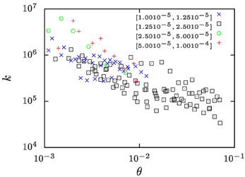
Figure 8. The k-values for the water-rich phase of water/iso-butoxyethanol mixtures as a function of the reduced temperature θ = (T − T_c)/T_c where T_c = 25.5°C is the critical temperature of the mixture. Different symbols refer to measurements where the volume-fraction growth rates, ξ, take values in the intervals indicated in the legend of the plot. The values of k have been calculated based on number densities n reported by Lapp et al. [25], and the other material parameter are extrapolations of the respective literature data which have been collected by Lapp [40].

Studies on other binary mixtures have addressed phase separation during a slow temperature ramp in differential scanning micro-calorimetry [24, 41] or by optical measurements [24, 42]. These experiments typically involve gradual changes of the temperature T by about 1 K/h, which amounts to ξ in the range also explored by Lapp et al. [25]. Hence, we expect that they involve similarly large values of k.

6.2. Growth of Cloud Droplets

Rain emerges when the air masses in a cloud rise due to topographic constraints, or by encountering a cold front [43, 44]. The drop of pressure in response to the rising of height H leads to adiabatic cooling of the air. This in turn changes the solubility of water in the air. Similarly to the phase separation discussed in Section 6.1 this induces a continuous growth of cloud droplets until they reach a size where collisions due to gravity and inertia speed up their growth and trigger rain formation [45]. Clement [46] discussed the micro-physics of the droplet growth, emphasizing the importance of the heat of condensation and the impact of solutes in the droplets.

Here we augment his study by an estimate of the possible impact of the continuous growth of the droplet volume fraction. We note that ξ amounts to the product of three factors,

$\xi =\frac{\text{d}\Phi }{\text{d}t}=\frac{\text{d}\Phi }{\text{d}T}\frac{\text{d}T}{\text{d}H}\frac{\text{d}H}{\text{d}t},$

where Φ = V/ is the volume fraction of droplets. The three factors on the right hand side of the equation amount to the slope of the phase boundary,¹ dΦ/dT ≲ 5· 10⁻⁴ K⁻¹ [47, p. 132], the adiabatic lapse rate dT/dH ≃ 1 K/100 m ([47, p. 148] or [44, p. 29]), and the average upwind speeds, dH/dt = 1 … 10 m/s, respectively. This gives rise to values of ξ between 5· 10⁻⁶s⁻¹ and 5· 10⁻⁵s⁻¹.

The number density of droplets in a cloud has been determined by Ditas et al. [48] in recent measurement campaigns, n = 4.7· 10⁸m⁻³, and the diffusion constant and the Kelvin length are well-known material constants. The latter is obtained by inserting the values of the interfacial tension of the water-air interface, γ, the molar volume of liquid water, V_m = 18 · 10⁻⁶ m³/mol, [43, p. 614], the equilibrium volume faction of water vapor in air, Φ, the molar gas constant, R = 8.3 J/mol K, and the temperature T into the definition of the Kelvin length [26]

$\begin{array}{cc}\sigma =\frac{2\gamma V_m\Phi }{RT}.& \left(34\right)\end{array}$

In Table 1 we provide some representative data and the resulting values for ξ and k. For average vertical wind speeds of 1 m/s the values of k lie in the range of 5 … 8, and for larger wind speeds higher values are obtained.

TABLE 1

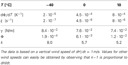
Table 1. Material constants for mixtures of water and air, and the resulting values for ξ and k.

We stress that the values provided in Table 1 provide only a rough, first order estimate of the parameters governing the evolution of the droplet size distribution in clouds. Nevertheless, this estimate suggests that the droplet volume growth due to the average rising of a cloud can give rise to values of k in the range k ≳ 5 where the present results promise the arising of interesting new physics. This calls for a careful revisiting of the pertinent droplet growth laws.

6.3. Synthesis of Monodisperse Colloids and Nano-Particles

Fundamental work on the synthesis of monodisperse colloids goes back to LaMer and Dinegar [14] and Reiss [15]. The theoretical understanding of the mechanisms that lead to highly monodisperse colloids and nano-crystals is still a topic of active research [17, 49, 50].

For the synthesis of monodisperse silver particles (used for photographic films) the material flux is well defined, and all material constants required to determine the k-values have been documented. For the synthesis of Ag Br and Ag Cl particles Sugimoto and coworkers [51, 52] provided material constants and aggregate numbers that allow us to calculate k based on the increase of the total volume of the aggregates, ξ, the diffusion coefficient D, and the Kelvin length σ,

$\begin{array}{cc}k=1+\frac{\xi }{4\pi D\sigma n}=1+\frac{Q_0{V}_m}{4\pi D\sigma N},& \left(35\text{a}\right)\end{array}$

where N is the number of aggregates in the sample volume , and

is provided in terms of the molar volume, V_m, and the mass supply rate, Q₀. Finally, the specific surface energy γ, the buffer temperature T, the mean-field monomer concentration C_∞, and the molar gas constant R = 8.314 J/(mol K) provide the Kelvin length as

$\begin{array}{cc}\sigma =\frac{2\gamma V_m^2{C}_{\infty }}{RT}.& \left(35\text{c}\right)\end{array}$

Table 2 provides the resulting k-values for different representative sets of (T, D, C_∞, N) used for the synthesis of Ag Br particles, and Table 3 provides the k values for the synthesis of Ag Cl particles. Also in the latter case the k values are obtained from Equations (35), except that Sugimoto et al. [52] provided the molar injection rate q₀ = Q₀/ and the number density of particles, n = N/.

TABLE 2

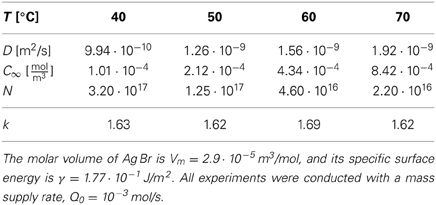
Table 2. Representative material parameters for the synthesis of monodisperse Ag Br particles [adapted from 51] and the corresponding k values as calculated via Equations (35).

TABLE 3

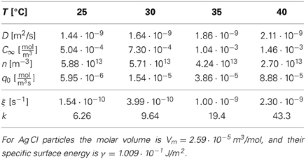
Table 3. Material parameters for the synthesis of monodisperse Ag Cl particles [adapted from 52, Table 3], and the resulting k-values as calculated via Equations (35).

The data show that the k values selected for the synthesis of monodisperse silver particles lie at k≃ 1.6 for Ag Br-particles and in a range between 6 and 43 for Ag Cl. Moreover, for the initial stages of the synthesis of Cd Se nano-crystals Clark et al. [17] estimated k to lie in the range of k ≃ 3 … 5 (see their Figure 4). These choices have been obtained by tuning the temperature and the rates Q₀ or q₀ for optimal monodispersity of the product. In all cases this resulted in k values larger than 3/2 such that one can profit from the size focusing arising for k > 3/2. In principle, the values of k should be chosen as large as possible to achieve the smallest standard deviation, Equation (33), and minimize the time required for the synthesis, Equation (4). In practice, it becomes harder to realize stable and reproducible experimental conditions for large values of k, and the heat released in the growth might severely alter the present theory for large growth rates. Follow-up work will have to explore these effects.

7. Conclusion

In Equations (1) we have identified the dimensionless factor k as control parameter determining the features of the evolution of an aggregate distribution evolving with overall volume growth. For k = 1 (i.e., no growth) the dynamics recovers the Lifshitz-Slyozov-Wagner scenario of Ostwald ripening [5, 8]. For 1 < k < 3/2 we expect Ostwald-like behavior as described by Slezov [6, Chapter 7]. In the present paper we focused on the case k > 3/2. On the one hand, we established a new numerical algorithm, that is outlined in Figure 2. It allows us to accurately follow the evolution of the aggregate size distribution over very long times because it admits equidistant time stepping on a logarithmic time axis. On the other hand, we have provided a complete analytical solution for the evolution of the aggregate size distribution. Our prediction has no adjustable parameters and agrees perfectly with the numerical data.

This excellent agreement establishes that for k > 3/2 the CDF does not approach a scaling form. Rather it is most conveniently written as a function of the difference, R² − 〈R²〉, of the square of the considered radius, R, and its average, 〈R²〉. We demonstrated in Figure 7 that to a very good approximation the shape of the distribution function remains invariant when this dependence is augmented by a gradual broadening by a factor 〈R〉^1/(k−1). Sub-dominant contributions to the evolution can arise from small aggregates that grow slightly slower than those of average size. They lead to noticeable changes in the small-size tail of the distribution for k ≲ 10. The resulting change of the shape of the distribution can be accounted for by considering the higher order correction in Equation (29a) and by self-consistently tracking the influence of the evaporation of aggregates. The resulting parameter-free prediction provides an excellent description of the asymptotic shape of the distribution (dotted gray lines in Figure 7). Consequently, the shape of the aggregate size distribution is fully determined by its initial condition, rather than by features of the dynamics.

In conclusion we have established that a weak thermal drift, or any other mechanism that leads to slow aggregate growth, can have dramatic effects on the aggregate size distribution. Even for very small effective driving it has a noticeable impact on various features of the aggregate size distribution.

The aggregate number density is constant at late times (see Figure 6). In contrast to this finding for k > 1, the ripening in isothermal systems (i.e., for k = 1) can only evolve by evaporation of small aggregates. This leads to a t⁻¹ decay of the number of aggregates.

The mean aggregate radius grows like 〈R〉 ~ t^1/3. In contrast to Ostwald ripening, this growth is not connected to the evaporation of aggregates, but reflects the growth due to a constant volume flux onto the aggregates at a fixed number of aggregates.

The standard deviation of the aggregate radius decays with the non-trivial power (t^1/3)^{−1+1/(k−1)} [cf. Equation (33)]. Consequently, the relative width of the distribution, which amounts to the ratio of the standard deviation and the average radius, 〈R〉, decays like (t^1/3)^{−2+1/(k−1)}. The aggregate size distribution tends to become more and more monodisperse.

The shape of the distribution is governed by initial conditions, rather than being universal. When plotted as a function of $\tilde{x}$ specified by Equation (30) the cumulative distribution function remains invariant except for small k where there is a slight change of the tails. This change has been accounted for in the theoretical prediction shown by the dotted gray lines in Figure 7.

The latter two findings are in striking contrast to those of the Lifshitz-Slyozov-Wagner theory of Ostwald ripening, which predicts that the distribution approaches a universal distribution with a fixed relative width.

For a range of different applications we have demonstrated in Section 6 that values of k > 3/2, where these differences prominently apply, may be regarded as common rather than as an exception. Consequently, the theory for the aggregate size distributions, that we have established in Section 5, opens new opportunities in the characterization and synthesis of aggregate growth. On the one hand, one can use the growth as a microscope to infer the initial size distribution at nucleation from a measurement at a later time when the aggregates have grown to a larger size. On the other hand, the distinct dependence of the size distribution on the initial conditions can be exploited to generate assemblies of aggregates with tailored size distributions. Moreover, in situations where k shows a non-trivial evolution in time the present theory provides a more natural starting point for an analysis of the aggregate growth than the Lifshitz-Slyozov-Wagner theory, because according to Equation (1) the point k = 1 is unstable with respect to growth of k when n decreases due to the evaporation of aggregates.

Conflict of Interest Statement

The authors declare that the research was conducted in the absence of any commercial or financial relationships that could be construed as a potential conflict of interest.

Acknowledgments

We acknowledge feedback by Karl-Henning Rehren upon developing the present theory, and inspiring discussions with Markus Abel, Bernhard Altaner, Nicolas Rimbert, Artur Wachtel, and Michael Wilkinson. Lucas Goehring, Stephan Herminghaus, and Artur Wachtel provided feedback on the manuscript.

Footnotes

1. ^It has been demonstrated by Lapp et al. [25] that dΦ/dT amounts to the slope of the binodal line of the phase diagram.

References

1. Wagner C. Theorie der Alterung von Niederschlägen durch Umlösen (Ostwald-Reifung). Z Elektrochemie (1961) 65:581–591.

2. Kahlweit M. On the kinetics of precipitation. Faraday Disc. (1976) 61:48–52. doi: 10.1039/dc9766100048

CrossRef Full Text

3. Johnson NJ, Korinek A, Dong C, Veggel FC. Self-focusing by Ostwald ripening: a strategy for layer-by-layer epitaxial growth on upconverting nanocrystals. J Am Chem Soc. (2012) 134:11068–71. doi: 10.1021/ja302717u

Pubmed Abstract | Pubmed Full Text | CrossRef Full Text

4. Lifshitz IM, Slyozov VV. The kinetics of precipitation from supersaturated solid solutions. J Phys Chem Solids (1961) 19:35–50. doi: 10.1016/0022-3697(61)90054-3

CrossRef Full Text

5. Bray AJ. Theory of phase-ordering kinetics. Adv Phys. (1994) 43:357–459. doi: 10.1080/00018739400101505

CrossRef Full Text

6. Slezov VV. Kinetics of First-Order Phase Transitions. Weinheim: Wiley-VCH (2009). doi: 10.1002/9783527627769

CrossRef Full Text

7. Shneidman VA. Early stages of Ostwald ripening. Phys Rev E (2013) 88:010401. doi: 10.1103/PhysRevE.88.010401

Pubmed Abstract | Pubmed Full Text | CrossRef Full Text

8. Voorhees PW. The theory of Ostwald ripening. J Stat Phys. (1985) 38:231–52. doi: 10.1007/BF01017860

CrossRef Full Text

9. Penrose O. The Becker-Döring equations at large times and their connection with the LSW theory of coarsening. J Stat Phys. (1997) 89:305–20. doi: 10.1007/BF02770767

CrossRef Full Text

10. Niethammer B, Pego RL. Non-self-similar behavior in the LSW theory of Ostwald ripening. J Stat Phys. (1999) 95:867–902. doi: 10.1023/A:1004546215920

CrossRef Full Text

11. Smereka P. Long time behavior of a modified Becker-Döring system. J Stat Phys. (2008) 132:519–33. doi: 10.1007/s10955-008-9552-9

CrossRef Full Text

12. Goudon T, Lagoutiére F, Tine LM. The Lifschitz-Slyozov equation with space-diffusion of monomers. Kinet Relat Models (2012) 5:325–55. doi: 10.3934/krm.2012.5.325

CrossRef Full Text

13. Ostwald W. Über die vermeintliche Isomerie des roten und gelben Quecksilberoxyds und die Oberflächenspannung fester Körper. Z Phys Chem. (1900) 34:495–503.

14. LaMer VK, Dinegar RH. Theory, production and mechanism of formation of monodispersed hydrosols. J Am Chem Soc. (1950) 72:4847–54. doi: 10.1021/ja01167a001

CrossRef Full Text

15. Reiss H. The growth of uniform colloidal dispersions. J Chem Phys. (1951) 19:482–87. doi: 10.1063/1.1748251

CrossRef Full Text

16. Kwon SG, Hyeon T. Formation mechanisms of uniform nanocrystals via hot-injection and heat-up methods. Small (2011) 7:2685–702. doi: 10.1002/smll.201002022

Pubmed Abstract | Pubmed Full Text | CrossRef Full Text

17. Clark MD, Kumar SK, Owen JS, Chan EM. Focusing nanocrystal size distributions via production control. Nano Lett. (2011) 11:1976–80. doi: 10.1021/nl200286j

Pubmed Abstract | Pubmed Full Text | CrossRef Full Text

18. Sowers KL, Swartz B, Krauss TD. Chemical mechanisms of semiconductor nanocrystal synthesis. Chem Mater. (2013) 25:1351–62. doi: 10.1021/cm400005c

CrossRef Full Text

19. Barenblatt GI. Scaling, Cambridge Texts in Applied Mathematics. Cambridge, NY: Cambridge UP (2003).

20. Vollmer J, Vollmer D, Strey R. Oscillating phase separation in microemulsions II: description by a bending free energy. J Chem Phys. (1997) 107:3627–33. doi: 10.1063/1.474720

CrossRef Full Text

21. Cates ME, Vollmer J, Wagner A, Vollmer D. Phase separation in binary fluid mixtures with continuously ramped temperature. Philos Trans R Soc Lond A (2003) 361:793–807. doi: 10.1098/rsta.2002.1165

Pubmed Abstract | Pubmed Full Text | CrossRef Full Text

22. Vollmer J, Auernhammer GK, Vollmer D. Minimal model for phase separation under slow cooling. Phys Rev Lett. (2007) 98:115701. doi: 10.1103/PhysRevLett.98.115701

Pubmed Abstract | Pubmed Full Text | CrossRef Full Text

23. Nozawa K, Delville M, Ushiki H, Panizza P, Delville J. Growth of monodisperse mesoscopic metal-oxide colloids under constant monomer supply. Phys Rev E (2005) 72:011404. doi: 10.1103/PhysRevE.72.011404

Pubmed Abstract | Pubmed Full Text | CrossRef Full Text

24. Auernhammer GK, Vollmer D, Vollmer J. Oscillatory instabilities in phase separation of binary mixtures: fixing the thermodynamic driving. J Chem Phys. (2005) 123:134511. doi: 10.1063/1.2046608

Pubmed Abstract | Pubmed Full Text | CrossRef Full Text

25. Lapp T, Rohloff M, Vollmer J, Hof B. Particle tracking for polydisperse sedimenting droplets in phase separation. Exp Fluids (2012) 52:1187–200. doi: 10.1007/s00348-011-1243-7

CrossRef Full Text

26. Landau LD, Lifshitz EM. Lehrbuch der Theoretischen Physik, Vol. 10. Physikalische Kinetik. Berlin: Akademie (1983).

27. Jana S, Srivastava BB, Pradhan N. A controlled growth process to design relatively larger size semiconductor nanocrystals. J Phys Chem C (2013) 117:1183–8. doi: 10.1021/jp310783a

CrossRef Full Text

28. Ludwig F-P, Schmelzer J. Cluster formation and growth in segregation processes with constant rates of supply of monomers. Z Phys Chem. (1995) 192:155–67. doi: 10.1524/zpch.1995.192.Part-2.155

CrossRef Full Text

29. Sugimoto T. Preparation of monodispersed colloidal particles. J Coll Inter Sci. (1987) 28:65–108. doi: 10.1016/0001-8686(87)80009-X

CrossRef Full Text

30. Peng X, Wickham J, Alivisatos AP. Kinetics of II-VI and III-V colloidal semiconductor nanocrystal growth: “focusing” of size distributions. J Am Chem Soc. (1998) 120:5343. doi: 10.1021/ja9805425

CrossRef Full Text

31. Soltzberg LJ, Bowers PG, Hofstetter C. A computer model for soda bottle oscillations: “the bottelator.” J Chem Educ. (1997) 74:711–4. doi: 10.1021/ed074p711

CrossRef Full Text

32. Zhang Y, Xu Z. “Fizzics” of bubble growth in beer and champagne. Elements (2008) 4:47–9. doi: 10.2113/GSELEMENTS.4.1.47

CrossRef Full Text

33. Ingebritsen SE, Rojstaczer SA. Controls on geyser periodicity. Science (1993) 262:889–92. doi: 10.1126/science.262.5135.889

Pubmed Abstract | Pubmed Full Text | CrossRef Full Text

34. Toramaru A, Maeda K. Mass and style of eruptions in experimental geysers. J Volcanol Geother Res. (2013) 257:227–39. doi: 10.1016/j.jvolgeores.2013.03.018

CrossRef Full Text

35. Han WS, Lu M, McPherson BJ, Keating EH, Moore J, Park E, et al. Characteristics of CO₂ -driven cold-water geyser, crystal geyser in Utah: experimental observation and mechanism analyses. Geofluids (2013) 13:283–97. doi: 10.1111/gfl.12018

CrossRef Full Text

36. Manga M. Waves of bubbles in basaltic magmas and lavas. J Geophys Res. (1996) 101:17457–65. doi: 10.1029/96JB01504

CrossRef Full Text

37. Sparks RS, Huppert HE. The origin of granites. Nature (1987) 330:207–8. doi: 10.1038/330207a0

CrossRef Full Text

38. Martin D, Nokes R. Crystal settling in a vigorously converting magma chamber. Nature (1988) 332:534–6. doi: 10.1038/332534a0

CrossRef Full Text

39. Vollmer J. Phase separation under ultra-slow cooling: onset of nucleation. J Chem Phys. (2008) 129:164502. doi: 10.1063/1.2989797

Pubmed Abstract | Pubmed Full Text | CrossRef Full Text

40. Lapp T. Evolution of Droplet Distributions in Hydrodynamic Systems, Ph.D. Thesis. Georg August University Göttingen and – Göttingen Graduate School for Neurosciences, Biophysics, and Molecular Biosciences Göttingen (2011). Available online at: http://hdl.handle.net/l1858/00-1735-0000-0006-B54l-8

41. Heimburg T, Mirzaev SZ, Kaatze U. Heat capacity behavior in the critical region of the ionic binary mixture ethylammonium nitrate–n-octanol. Phys Rev E (2000) 62:4963–7. doi: 10.1103/PhysRevE.62.4963

Pubmed Abstract | Pubmed Full Text | CrossRef Full Text

42. Rullmann M, Alig I. Scaling behavior of nonisothermal phase separation. J Chem Phys. (2004) 120:7801–10. doi: 10.1063/1.1687320

Pubmed Abstract | Pubmed Full Text | CrossRef Full Text

43. Mason BJ. The Physics of Clouds. 2nd Edn, Oxford Monographs on Meterology. New York, NY: Oxford University Press (1971).

44. Rogers RR, Yau MK. A Short Course in Cloud Physics, 3rd Edn. International Series in Natural Philosophy. Vol. 113 Oxford: Pergamon Press (1989).

45. Bodenschatz E, Malinowski SP, Shaw RA, Stratmann F. Can we understand clouds without turbulence? Science (2010) 327:970–1. doi: 10.1126/science.1185138

Pubmed Abstract | Pubmed Full Text | CrossRef Full Text

46. Clement CF. Mass transfer to aerosols. In: Colbeck I, ed. Environmental Chemistry of Aerosols. Oxford: Blackwell Publishing Ltd (2009). p. 49–89.

47. Moran JH, Morgan MD. Meteorolgy: The Atmosphere and the Science of Weather, 5th Edn. Upper Saddle River, NJ: Prentice-Hall (1997).

48. Ditas F, Shaw RA, Siebert H, Simmel M, Wehner B, Wiedensohler A. Aerosols-cloud microphysics-thermodynamics-turbulence: evaluating supersaturation in a marine stratocumulus cloud. Atm Chem Phys. (2012) 12:2459–68. doi: 10.5194/acp-12-2459-2012

CrossRef Full Text

49. Rempel JY, Bawendi MG, Jensen KF. Insights into the kinetics of semiconductor nanocrystal nucleation and growth. J Am Chem Soc. (2009) 131:4479-89. doi: 10.1021/ja809156t

Pubmed Abstract | Pubmed Full Text | CrossRef Full Text

50. Singh A, Puri S, Dasgupta C. Growth kinetics of nanoclusters in solution. J Phys Chem B (2012) 116:4519–23. doi: 10.1021/jp211380j

Pubmed Abstract | Pubmed Full Text | CrossRef Full Text

51. Sugimoto T. The theory of the nucleation of monodisperse particles in open systems and its application to AgBr systems. J Coll Inter. Sci. (1992) 150:208–25. doi: 10.1016/0021-9797(92)90282-Q

CrossRef Full Text

52. Sugimoto T, Shiba F, Sekiguchi T, Itoh H. Spontaneous nucleation of monodisperse silver halide particles from homogeneous gelatin solution I: silver chloride. Coll Surf A Physchem Eng Aspects (2000) 164:183–203. doi: 10.1016/S0927-7757(99)00366-0

CrossRef Full Text