Efficient event-driven simulations shed new light on microtubule organization in the plant cortical array

1. Introduction

A key distinguishing feature between animal and plant cells is the cellulosic cell wall that encases the latter. This extracellular structure confers on plant cells the mechanical strength to withstand their significant internal osmotic pressure. The presence of the semi-rigid cell wall also imposes a much more defined shape on plant cells in comparison to animal cells. This in turn poses a special challenge to a plant cell, namely how to grow without losing mechanical integrity and how to control the cell geometry during growth. Strikingly, thinking about how these requirements could be met led Paul Green to deduce, as early as 1962 [1], that cells must possess filamentous structures with the ability to form parallel-organized arrays, effectively “predicting” the existence of microtubules a year before they were first positively identified. Indeed, we now know that in growing plants cells microtubules are a key regulator of cell expansion. They do so by forming the so-called transverse cortical array.

This array consists of microtubules that are physically associated to the cytoplasmic side of the plasma membrane and statistically aligned in a preferential orientation transverse to the growth axis of the cell (3; see Figure 1). The current understanding is that this array determines the insertion [4] and the subsequent direction of motion of cellulose synthase complexes that deposit cellulose microfibrils into the cell wall [5]. Cellulose microfibrils are the load-bearing elements of the cell wall and their organized deposition confers the required anisotropic mechanical properties to the wall that enable its controlled expansion. Live cell imaging revealed that cortical microtubules can collide [6, 7]. The outcome of these collisions is partly stochastic and depends on the angle between the incoming growing microtubule and the obstructing microtubule (7; see Figure 2). At small collision angles the most likely outcome is zippering, where the incoming microtubule bends to continue growing along the obstructing microtubule. At increasingly perpendicular collision angles a so-called induced catastrophe becomes more prevalent, in which the incoming microtubule switches to the shrinking state. The remaining possibility is that the incoming microtubule slips over the obstructing microtubule in what is called a cross-over.

FIGURE 1

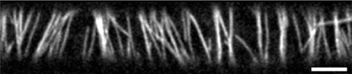
Figure 1. Cortical microtubule array in 3 day old dark grown epidermal hypocotyl cell. Microtubules are labeled by mCherry-TUA5. For information about plant material and microscopy settings see Lindeboom et al. [2]. Scale bar is 5 μm.

FIGURE 2

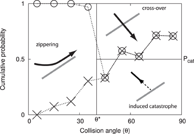
Figure 2. Angle dependent outcomes of microtubule collisions. Graphical depiction of the microtubule interaction model, expressed as cumulative probabilities as a function of the interaction angle θ. The experimental data by Dixit and Cyr [7] are indicated using dashed lines and symbols: induced catastrophes below the crosses, cross-overs above the circles and zippering in between.

The first full-fledged attempt to simulate cortical array ordering is due to Baulin et al. [8], who considered a minimal model for collision-induced ordering of 2D dynamical filaments, which abstracted from the full complexity of stochastic microtubule dynamics, and replaced the actual interactions by collision-induced pausing of otherwise deterministically growing microtubules. More recently, three groups almost simultaneously published computational approaches toward understanding cortical array organization, including realistic microtubule dynamics. Allard et al. [9] presented results on simulations with microtubule dynamical parameters taken from observations on wild-type and MOR1-mutant Arabidopsis thaliana cells and a simplified collision scheme with 100% zippering below a critical incidence angle θ* and fixed ratio of induced catastrophes versus cross-overs above this angle. The simulations were carried out on a two dimensional surface with either periodic or catastrophe-inducing boundary conditions, using an event-driven algorithm for individual microtubule dynamics and a fixed time-step algorithm for the detection of collisions. Eren et al. [10] presented simulations on cylindrical surfaces in 3-dimensions, using an event-driven simulation method. Because of the restrictive cylindrical system without end caps, these were effectively 2-dimensional simulations with periodic boundary conditions in one direction, and either catastrophe inducing or a type of reflective boundary conditions in the other direction. The collision dynamics and microtubule dynamical parameters were similar to that of Allard et al. Finally, in our own work [11] we employed an event-driven simulation technique to study two-dimensional systems with periodic boundary conditions, including comparisons with the theoretical model presented in Hawkins et al. [12].

Here we present the first detailed description of our simulation method as well as some novel applications. Our method has three important features: First of all, it employs a highly efficient event-driven algorithm making it possible to perform fast and, in principle, exact simulations, outperforming finite time step simulations by a wide margin. Next, it leverages the results of our previous theoretical analysis by employing a single control parameter G_c to select distinct states of the system, dramatically reducing the number of independent parameters to consider. Finally, it provides an integrated framework for simulating and analyzing cortical microtubule dynamics on closed and curved surfaces, including a number of key biological processes which have been identified to influence this behavior.

We then address several key conceptual issues in modeling and understanding interacting cortical microtubules. We start by presenting a cross-validation of the simulations with our previously presented theoretical analysis based on mean-field assumptions. Next, we address how a finite pool of tubulin can stabilize systems whose dynamical parameters suggest that the microtubules are in the so-called unbounded growth regime, which appears to be the case for a number of experimental data sets that have been discussed in the literature. The question of whether induced catastrophes alone are a sufficient cause of ordering, or whether zippering is necessary or even sufficient by itself appears as an open debate in the current literature [e.g., compare 13, 14]. Here, we present an extensive analysis of the complex interplay between induced catastrophes, zippering and microtubule minus-end treadmilling, which shows, among others, that zippering is neither necessary nor sufficient to induce an ordering transition. Finally, we consider the influence of cell geometry and of local disturbances in microtubule dynamics on the alignment and the orientation of the cortical array.

2. Model for Microtubule Dynamics and Interactions

At the microscopic level, the formation of the cortical array is driven by the intrinsic dynamics of microtubules and by microtubule interactions. Here we describe how these are incorporated into our simulation model.

2.1. Intrinsic Dynamics

We assume that microtubules are nucleated with a random position and orientation according to a nucleation rate r_n. Once nucleated, the intrinsic dynamics of the plus end are governed by the two-state model introduced in Dogterom and Leibler [15]. In the growing (+) state, the microtubule extends at its plus end with speed v⁺ and in the shrinking (−) state it retreats with speed v⁻. Microtubules spontaneously switch from the growth to the shrinkage state (a so-called “catastrophe”) with a rate r_c (per microtubule), and the reverse process (a “rescue”) occurs with a rate r_r. On the opposite end of the microtubule, the minus end optionally retreats with a treadmilling speed v^tm [6].

In addition to these microtubule-intrinsic factors we also include microtubule severing. In plants the microtubule severing enzyme katanin is responsible for detaching microtubules from their nucleation complex [16] and for severing at microtubule crossovers [2]. Here we limit ourselves to delocalized severing, which we model through a constant severing rate r_s per unit length. Severing is taken to be instantaneous and results in the formation of two new microtubule ends—plus and minus—at the severing location. The newly created plus-end immediately undergoes a catastrophe, which places it in the shrinking state.

The default parameters used for the simulations in this work are identical to those used in Deinum et al. [17] and are listed in Table 1. As in that paper, we modulate the catastrophe rate to achieve different values of the control parameter G_c (see section 4.1). Although microtubule severing is included in the simulation model and accompanying tools, the effect of severing is not illustrated in this paper, hence r_s = 0 for all simulations.

TABLE 1

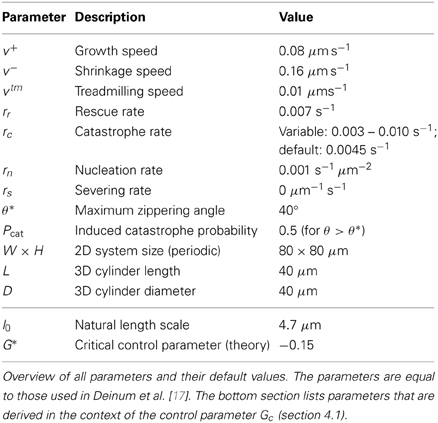
Table 1. Simulation parameters.

2.2. Microtubule Interactions

When a growing microtubule plus end collides with another microtubule, the outcome is a function of the collision angle θ ∈ (0, 90°]. We follow the simplified interaction model first introduced in Allard et al. [9], and also used by Eren et al. [10]; see Figure 2. When the collision angle θ ≤ θ* = 40°, the collision results in zippering, causing the plus end to reorient alongside the encountered microtubule. For θ > θ*, the outcome is stochastic with equal odds for an induced catastrophe and a cross-over (i.e., no effect).

The zippering process (and occasionally the severing process) results in the formation of microtubule bundles. In the simulation model we assume that microtubules in a bundle coalesce and that a collision of an incoming growing microtubule tip with bundle is no different than a collision with a single microtubule. Similarly, a microtubule that is part of a bundle is not affected by the presence of other microtubules within that bundle when it collides with another microtubule. An exception is made in section 5.2, where we consider convergence to mean-field theoretical results in the weak interaction limit. In this limit, the interaction probabilities must be taken proportional to the number of microtubules in a bundle. Finally, we note that other bundle interaction models are conceivable, and some of these have been explored in Tindemans [18].

2.3. Finite Tubulin Pool

The microtubule dynamic model defined above assumes that the dynamic parameters are constant in time. Particularly, the use of a constant growth speed implies that the supply of tubulin dimers that can be used to elongate microtubules is effectively infinite. Cells do not have such an infinite supply of tubulin, and it is worthwhile to consider the effects of a limited pool of tubulin. The depletion of free tubulin (i.e., not currently incorporated in microtubules) will primarily affect the rate at which tubulin dimers polymerize on growing microtubule tips. This effect is linear to a first approximation [19], and we therefore include the finite tubulin pool in our model using a length-dependent growth rate

$\begin{array}{cc}{v}^{+}(t)=v_0^{+}\left(1-\frac{L(t)}{L_{\text{max}}}\right),& \left(1\right)\end{array}$

where L(t) is the total length of the microtubules in the system, and L_max is the length-equivalent of the total amount of tubulin in the system. This way, the total microtubule length is bounded by L_max. In practice, the size of the tubulin pool is best specified via a mean length-equivalent tubulin concentration ρ_tub so that L_max = ρ_tubA, where A is the total surface area of the cell. Note that a more complete implementation would also consider the effects of the available tubulin concentration on nucleation, which we keep constant.

The varying plus end growth speed has implications for the computation of event times in our event-driven simulation scheme. This will be discussed in section 3.2 and is further elaborated in the Supplementary Materials. The effect of a limited tubulin pool on the simulation results is discussed in section 5.3.

2.4. The Inclusion of a Pause State

In the present work we have only considered the classical two-state model of microtubule plus-end dynamical instability. In reality microtubule plus-ends also display pause states, and both Allard et al. [9] and Eren et al. [10] have chosen to explicitly take these into account in their simulations. A legitimate question is thus whether and, if so, to what extent this difference is important for understanding the behavior of these systems. Here we argue that this is not the case. This can be understood on a heuristic level by considering that the presence of paused states only influences the dynamics in between the significant events (nucleation, collisions, leaving a bundle by shrinking, or shrinking to zero length) that determine the ultimate state of the system, but has no direct impact on these events. This means that microtubule pausing may affect the kinetics of the model, by affecting the mean waiting time between events, but not the steady state behavior.

In the Supplementary Material section 1 we formally construct an exact mapping between the three-state microtubule instability model and a corresponding two-state model with exactly the same predictions for the mean length and mean lifetime of a single isolated microtubule. This same mapping moreover induces an exact correspondence between a three-state mean-field theory and the two-state theory developed in Hawkins et al. [12], implying that the predicted phase behavior of both theories will be identical.

The resulting correspondence is as follows. In the three-state model the microtubules can either grow (+) with speed v⁺, shrink (−) with speed v⁻ or pause (p). Microtubules can either switch directly from the growing to the shrinking state or vice-versa with rates f₊₋ and f₋₊, respectively, or switch from these states into the paused state with rates f_+p and f_−p, and exit from the latter state with rates f_p+ and f_p−. We can now define the effective growth and shrinkage speeds

$\begin{array}{cc}{\tilde{v}}^{-}=\frac{\left(f_{p+}+f_{p-}\right)}{\left(f_{-p}+f_{p+}+f_{p-}\right)}{v}^{-}& \left(2\right)\end{array}$

$\begin{array}{cc}{\tilde{v}}^{+}=\frac{\left(f_{p+}+f_{p-}\right)}{\left(f_{+p}+f_{p+}+f_{p-}\right)}{v}^{+}& \left(3\right)\end{array}$

and catastrophe and rescue rates

$\begin{array}{cc}{\tilde{r}}_c=\frac{\left(f_{+p}{f}_{p-}+f_{+-}{f}_{p+}+f_{+-}{f}_{p-}\right)}{\left(f_{+p}+f_{p+}+f_{p-}\right)}& \left(4\right)\end{array}$

$\begin{array}{cc}{\tilde{r}}_r=\frac{\left(f_{p+}{f}_{-+}+f_{p+}{f}_{-p}+f_{p-}{f}_{-+}\right)}{\left(f_{-p}+f_{p+}+f_{p-}\right)}& \left(5\right)\end{array}$

which define the corresponding two-state model.

In view of these observations we conclude that the explicit inclusion of paused microtubule states in the simulations is not a crucial ingredient, and results for the phase behavior from the two approaches are readily compared by employing the above mentioned mapping to determine the equivalent dynamical parameter set.

2.5. Microtubule Trajectories on Curved Surfaces

What is the path that a cortical microtubule follows along a curved membrane? Depending on the specific constraints there are two types of solutions to this problem. When the microtubule is only confined by the cell membrane, but still free to move laterally, the solution is given by a global minimization of the curvature along the microtubule. This solution has been determined for an infinite cylinder—and, by extension, for spherocylinders—in Lagomarsino et al. [20] and is shown in Figure 4. As the filament becomes longer, its free end will tend to align more with the axis of the cylinder. However, the cortical microtubules in plant cells are linked to the cell membrane and are therefore restricted in their lateral movement [6, 21, 22]. This means that a microtubule cannot make use of lateral relaxation to decrease its bending energy as it extends. Instead, the polymerizing microtubule end can only locally minimize the bending energy before the curvature is “frozen in” by binding to membrane linkers. In this strongly bound limit the trajectory of growing microtubules is therefore given by a (locally) minimal curvature path on the cell membrane, starting from a given initial position and direction. It deserves mention that cortical microtubules are not actually attached to the cell membrane at all points along their length, but rather at intervals of a finite size [23–25], so there is some room for non-local curvature minimization. However, as long as the attachment interval is much smaller than the radius of the cylinder, the minimal curvature path is a good approximation.

The curvature κ of any regular curve on a surface can be decomposed into two components, the normal curvature κ_n in the normal plane (pointing out of the membrane) and the lateral curvature κ_l in the tangent plane (see Figure 3). These curvatures are related by

$\begin{array}{cc}{\kappa }^2={\kappa }_n^2+{\kappa }_l^2.& \left(6\right)\end{array}$

FIGURE 3

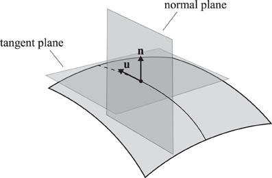
Figure 3. A trajectory on a two-dimensional curved surface. Indicated are the tangent vector u and the surface normal n. The normal plane contains both vectors and the tangent plane contains only the tangent vector and is perpendicular to the normal vector.

The Meusnier theorem states that for a given surface S, all possible curves through a certain point with a given tangent vector have the same normal curvature [26], so that any differences in curvature must be attributed to the lateral curvature κ_l. It follows from Eq. (6) that the total curvature is always minimized by setting κ_l = 0. This uniquely defines the continuation of a minimum curvature trajectory.

In this paper we will use flat-capped cylinders to represent the cell surface in three dimensions. The minimum curvature solutions on the surface of a cylindrical body are helices defined by their starting position and angle, which justifies the use of a wrapped periodic domain to represent a cylindrical surface. In Figure 4, the local and global curvature minimization solutions on the body of a cylinder are compared.

FIGURE 4

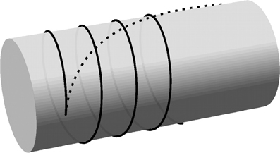
Figure 4. Curvature-minimizing trajectories on a cylinder. Trajectories resulting from local curvature minimization (solid line) and global curvature minimization (dashed line) are initiated from a single nucleation point with an initial opening angle of 5.7° from the transverse direction. The curve for the global energy minimization has a total length of 4.5 times the cylinder radius. (The length is not relevant for the helical solution resulting from local curvature minimization).

The minimal local curvature model for microtubule propagation is extended to the rim of the cylindrical cell as follows. The sharp transition from the cylinder body to the flat end caps is treated as the limiting case of a smooth edge with a vanishing radius of curvature. Locally, the rim of the cylindrical cell is approximately straight so that the smooth edge may be approximated by a (quarter section of) a cylinder with a vanishing radius. Mimimal curvature paths that traverse the edge are locally helical, which means they conserve the angle between the microtubule path and the edge of the cylindrical cell. The latter property is used in the simulations: when a microtubule reaches an edge of the cylindrical cell it continues on the neighboring face in the direction that preserves the angle between the microtubule and the edge.

3. Event-Driven Simulations

Implementing the cortical array model defined in the previous section in a computer simulation is not trivial, because the simulation method must accurately span a range of length scales (0.1–100 μm) and time scales (seconds −10 s of hours). In addition, because of the stochastic nature of the model, a large ensemble of simulations is required to assess the statistical properties of the outcomes for even a single initial condition.

A straightforward implementation with a fixed time step Δt would require very small time steps to deal with the micrometer and second scales, leading to unacceptably slow execution times. An event-driven simulation method is used instead to simulate the cortical array model in a way that does not introduce intrinsic uncertainties in the time domain and is thus both accurate and fast. The cortical array model exhibits two distinct types of dynamics: periods of continuous evolution (microtubule growth, shrinkage) interrupted by events (collisions, nucleations, etc.) that may trigger a discontinuous change in the system state. At any time, we can determine the time t_e at which the next event will take place. We then fast-forward the system state to t_e, update the microtubule lengths to reflect that time and process the event in question. This cycle is repeated until a predetermined end time is reached. This process is illustrated in Figure 5.

FIGURE 5

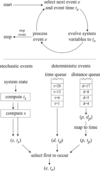
Figure 5. The event-driven simulation process. The top panel illustrates the event-driven simulation cycle. The bottom panel indicates how the first upcoming event is selected.

For computing the next event to take place we make a distinction between deterministic and stochastic events. Deterministic events are those events for which the event time is fully determined by the state of the system (collisions, disappearance, boundary conditions, simulation control), whereas stochastic events are the result of a random process (nucleations, spontaneous catastrophes, rescues, severing). The times corresponding to the next deterministic and stochastic events are computed using the methods outlined below and the event with the nearest time is executed.

3.1. Stochastic Events

Because all stochastic events are independent and described by simple rates (memoryless dynamics), we use a kinetic Monte Carlo algorithm [27] to determine the next stochastic event time, albeit with a potentially time-dependent event rate. Because of the memoryless property, we may recalculate Δt_stoch whenever it is (potentially) invalidated, such as after the execution of any deterministic event.

Each stochastic event type is associated with an event rate r_e(t). Most event rates are constant between events, with the exception of the severing rate, which is dependent on the total length of growing and shrinking microtubules. In particular,

$\begin{array}{cc}\begin{array}{l}R(t)=r_{\text{nucleation}}+r_{\text{spont}.\text{catastrophes}}+r_{\text{rescues}}\\ +r_{\text{severing}}\end{array}& \left(7\right)\end{array}$

$\begin{array}{cc}=r_{n}A+r_c{N}^{+}+r_r{N}^{-}+r_{s}L(t),& \left(8\right)\end{array}$

where A is the cell's surface area, N⁺ and N⁻ are the number of growing and shrinking microtubules, respectively, and L(t) is the total length of microtubules in the system. For a given rate, the time interval Δt_stoch to the next stochastic event follows from the expression

$\begin{array}{cc}{\displaystyle {\int }_t^{t+\Delta t_{\text{stoch}}}R}(t^{\prime })d{t}^{\prime }=-\log u,& \left(9\right)\end{array}$

where u is a uniform random variate on the interval (0, 1). The specific type of stochastic event that will take place may then be determined by selecting an event e at random in proportion to the corresponding rates r_e(t + Δt_stoch).

The simulations in section 5 were performed with r_s = 0, in which case R(t) is constant between events so that equation (9) produces

$\begin{array}{cc}\Delta t_{\text{stoch}}=-\frac{\log u}{R}.& \left(10\right)\end{array}$

The more general case for r_s ≠ 0 is addressed in Supplementary Material section 2.

3.2. Deterministic Events

The class of deterministic events includes collisions of microtubule plus ends with other microtubules or cell edges and the disappearance of microtubule segments because of retreating plus ends or treadmilling minus ends. Furthermore, the simulation makes use of deterministic “control” events to take measurements or snapshots at fixed time intervals, to update simulation parameters and to stop the simulation.

The efficiency of our simulations is greatly enhanced by the concepts of regions and trajectories. Where possible we partition the system geometry into regions with a span that is comparable to the natural length scale l₀ (see Eq. 12). Trajectories serve as “tracks” for microtubules. When a microtubule nucleates, a trajectory is created that spans the region as a minimum-curvature path tangential to the nucleation position and orientation. When a growing microtubule reaches the end of a trajectory at the region boundary, a new trajectory is computed as a continuation of the previous trajectory. If such a continuation already exists, that trajectory is used instead of creating a new one. Similarly, after a zippering event, the growing plus end switches trajectories to grow alongside the existing microtubule. The implication is that microtubules in a bundle always share a trajectory, which makes it easy to establish the number of microtubules in a bundle at a given location.

When a new trajectory is established its intersections with other trajectories in the same region are computed. These intersections are stored as an ordered list according to their distance along the trajectory. Because collisions between microtubules can only occur when their trajectories intersect, we may safely treat microtubules independently between trajectory crossings. The crossing events are therefore used as deterministic events in the simulation, and an actual collision only occurs if a microtubule is present on the trajectory that is being crossed. A further speedup is obtained by only updating a microtubule's position when it is involved in an event (such as a crossing of its trajectory) or when the system state is being analyzed for output (e.g., for a snapshot or order parameter calculation).

In this paper we consider only simulations on flat or cylindrical surfaces. In both cases the trajectories are straight lines in the appropriate representation, and the computation of their intersections is straightforward. However, the process outlined above is readily adapted to more general geometries. When a new trajectory is created, a minimum curvature path is created from the relevant starting orientation, using either analytical or numerical means appropriate to the geometry. Then the intersections with pre-existing trajectories in the same region are computed. Depending on the geometry this procedure may be involved, but it is robust against numerical errors because the intersections are only computed once. There is no scope for inconsistencies due to differences between subsequent evaluations.

For a given state of the system, deterministic events occur at a known time t_d in the future. This allows us to pre-compute the times at which deterministic events will take place and store them in a queue. At any given time, the front of the queue indicates the time interval Δt_det to the first deterministic event. In general, the occurrence of an event (both deterministic and stochastic types) will change the state of the system, causing new deterministic events to be added to the queue, or obsolete events to be invalidated.

A slight complication occurs with the inclusion of a finite tubulin pool cf. Eq. (1). In this case the speed of a growing plus end depends on the collective length of all microtubules in the system, which varies in unpredictable ways, making it impossible to precompute collision or boundary traversal times. For these plus-end associated events we create a second deterministic event queue. This queue does not store (and sort) events by their time of occurrence, but rather by the distance that a growing plus end must travel to arrive at the collision position. Because all plus ends are affected equally by the limited tubulin pool, their relative positions in the queue are conserved by the dynamics of the system. At any specific time t, the plus-end distance d_p corresponding to the first event can be meaningfully converted to an event time t_p. This can be compared to the event time from the other deterministic queue and the stochastic event time in order to determine the event that will occur first. This process is depicted in Figure 5, and the relevant equations are derived in Supplementary Material section 3.

4. Quantitative Analysis

Stochastic simulations of the cortical array make use of a large set of input parameters to generate a stochastic sequence of events representing the microtubule dynamics in the system. Formally, the simulation model represents a stochastic mapping from many input parameters to a dynamic pattern of interacting microtubules. Without additional structure the characterization of such a mapping to extract relevant knowledge is cumbersome.

However, on theoretical grounds we are able to condense the input and output to a small number of real-valued parameters. The microtubule dynamical parameters (see Table 1) are reduced to a single-valued control parameter G_c. On the output side, the microtubule patterns can be characterized in terms of the alignment order parameters R₂ (S₂ for planar systems) and the orientation angle Θ₂. The existence of these control and order parameters provides a convenient framework for analysis: measure the effect of G_c—and the few remaining input parameters not contained in G_c—on R₂ and Θ₂.

4.1. Control Parameter G_c

The theoretical work described in Tindemans et al. [11] and Hawkins et al. [12] has identified a control parameter G that can assist in the understanding of the simulation results, and clarify their dependence on the system parameters. In Deinum et al. [17] its definition was extended to include treadmilling microtubules, resulting in the control parameter

$\begin{array}{cc}\begin{array}{l}{G}_c={\left(\frac{2{(v^{+}-v^{tm})}^2(v^{-}+v^{tm})}{r_n{v}^{+}\left(v^{+}+v^{-}\right)}\right)}^{\frac{1}{3}}\times \\ \left(\frac{r_r}{v^{-}+v^{tm}}-\frac{r_c}{v^{+}-v^{tm}}\right)\end{array}& \left(11\right)\end{array}$

$\begin{array}{cc}\equiv l_0\times (-1/\overline{l}).(\text{for finite }\overline{l})& \left(12\right)\end{array}$

The control parameter can be expressed as the (negative) ratio of a natural length scale l₀ and the mean length l of microtubules in the absence of interactions. For the applications in section 5 we modulate G_c through the intrinsic catastrophe rate r_c. For the parameters in Table 1 we have

$\begin{array}{cc}{G}_c\approx -63.2\text{s} r_c+\mathrm{0.182.}& \left(13\right)\end{array}$

As noted in Deinum et al. [17], the G_c order parameter has a theoretical basis for the cases with either non-zero zippering or treadmilling (v^tm ≠ 0). Although a similar foundation is absent for the case with both zippering and treadmilling we extend the use of the control parameter G_c to include this case.

The value of G_c should be compared to the theoretical bifurcation value G*, which is fully determined by the angular probability P_cat(θ) to induce a catastrophe after a collision at angle θ.

$\begin{array}{cc}{G}^{*}={(-2{\widehat{c}}_2)}^{1/3}\left(\frac{{\widehat{c}}_0}{-2{\widehat{c}}_2}-1\right),& \left(14\right)\end{array}$

where ${\widehat{c}}_n$ is defined as

$\begin{array}{cc}{\widehat{c}}_n=\frac{4}{\pi }{\displaystyle {\int }_0^{\pi /2}\sin (\theta )\cos (n\theta )P_{\text{cat}}(\theta )}d\theta .& \left(15\right)\end{array}$

For the induced catastrophe probability used in this work (P_cat = 0.5 for angles larger than 40°), we have G* ≈ −0.15. The mean-field theory developed in Hawkins et al. [12] predicts that the system will remain in a disordered (isotropic) state if G_c ≤ G*, whereas it will align if G_c > G*. In biologically relevant cases, we have G* < 0. If in addition G_c > 0, the microtubules will align (as G_c > G*), but their density will continue increasing without bounds (unless tubulin depletion ultimately forces a sufficient decrease in G_c).

4.2. Order Parameters

4.2.1. Planar order parameter S₂

To measure the degree of alignment of the microtubules in a planar system, we use the microscopic (i.e., derived from the individual particles) order parameter S₂ from Deinum et al. [17]:

$\begin{array}{cc}\begin{array}{l}{S}_2=\left|{\langle {\text{e}}^{\text{i2}\theta }\rangle }_l\right|\text{=}\frac{|{\displaystyle {\sum }_n{l}_n}{\text{e}}^{\text{i2}{\theta }_{\text{n}}}\text{|}}{{\displaystyle {\sum }_n{l}_n}}\\ =\frac{\sqrt{{\left({\displaystyle {\sum }_n{l}_n}\cos 2{\theta }_n\right)}^2+{\left({\displaystyle {\sum }_n{l}_n}\sin 2{\theta }_n\right)}^2}}{{\displaystyle {\sum }_n{l}_n}},\end{array}& \left(16\right)\end{array}$

where the index n runs over the microtubule segments in the system, with length l_n and orientation angle θ_n. The S₂ order parameter has a value of 0 for an isotropic system and a value of 1 for a system in which the microtubules are all perfectly aligned. Note that this order parameter is insensitive to the polarity of the segments. This definition is identical to the order parameter S from Allard et al. [9], but does not require the intermediate determination of a dominant angle. In the limit of a system with very many microtubules, it is also equal to the mean-field definition used in Hawkins et al. [12].

4.2.2. Alignment on curved surfaces

The cell cortex is a curved surface embedded in three dimensions. The S₂ order parameter is defined only for planar systems, and when we attempt to apply it to curved surfaces we encounter two problems. First, it can only be used on systems such as the cylinder without end caps, where the surface can be “unrolled” to a simple 2D plane. The second issue is that even in that case it does not give valuable information about the orientation of the resulting pattern: for example, transverse and helical arrays can have the exact same value of S₂, even though they are qualitatively different.

To resolve these issues we have constructed a pair of 3D order parameters: R₂ and Θ₂. These parameters are rooted in the hypothesis that the formation of the cortical array is thought to serve the purpose of aligning the cellulose microfibrils in the cell wall, which in turn allows the cell wall to expand in the direction perpendicular to the microfibrils [28]. This sets two requirements on the cortical array: a sufficient degree of alignment and an orientation of the array perpendicular to the main expansion axis. The primary order parameter R₂ is an analog of S₂, and reduces to the same definition for a planar system. It has a value between 0 and 1, and measures the extent to which one can identify a common direction in 3D space that is perpendicular to the cortical microtubules. The secondary order parameter Θ₂ is specific to the cylindrical geometry and reports the angle between the preferential expansion axis and the main cylinder axis.

4.2.3. The tensorial order parameter

To measure the degree of order of the collective set of microtubules in the cell cortex, we recall the definition of the 3D nematic order parameter Q that is commonly used for liquid crystals [see e.g., 29]. It is a second order tensor (equivalent to a square matrix) that can be defined as

$\begin{array}{cc}Q=<u\otimes u>-\frac{1}{3}{I}^{(3)},& \left(17\right)\end{array}$

where ⊗ denotes the outer product of two vectors. In the case of discrete particles, u is the director of the individual particles in the system and the angled brackets denote an averaging over all particles. In the case of orientational density fields, u is the orientation and the brackets indicate a density-weighted average over all angles and space. The definition of Q is easily adjusted for a two-dimensional system, by reducing the dimensionality and replacing the fractions by 1/2. However, it is important to realize that in both of these cases the particles are free to position and orient themselves freely in the relevant space.

This is clearly not the case in the cortical array, where we have particles that are constrained by a two-dimensional surface S that is embedded in ℝ³, restricting the admissible orientations to the tangent plane at each location. This means that the surface geometry has a large, possibly non-isotropic, influence on the possible realizations of Q. This results in the problematic outcome that a homogeneous and locally isotropic configuration can give rise to non-zero elements in Q. To rectify this, we note that for the unconstrained 3D system, it is the identity matrix in (17) that ensures Q = 0 for any isotropic configuration. We generalize (17) by replacing the correction term $\frac{1}{3}{I}^{(3)}$ with a geometry-dependent correction term.

The following definitions will be given in terms of an orientational density field ρ(r, θ), where r ∈ S and θ is a coordinate indicating the orientation in the local tangent plane. The translation to a particle-based definition is straightforward, and will be given below. In terms of the orientational density field ρ, we define

$\begin{array}{cc}Q=<u\otimes u{>}_{\rho (r,\theta )}-<u\otimes u{>}_{\text{iso},\text{homo}}& \left(18\right)\end{array}$

$\begin{array}{cc}=<u\otimes u{>}_{\rho (r,\theta )}-T_{\text{geom}}.& \left(19\right)\end{array}$

Here, the first term is an average that is weighted by the actual orientation density field and the second is the isotropic correction term, where the averaging is done with respect to an isotropic and homogenous distribution. This correction is represented by the geometry-dependent tensor T_geom.

The isotropic homogeneous distribution tensor T_geom is defined as the result of two subsequent averaging procedures: first a local averaging over all directions in the tangent plane (isotropy) and then an averaging over r ∈ S (homogeneity). Defining a local orthogonal frame by the surface normal n and two orthogonal unit vectors v and w, the local averaging yields

$\begin{array}{cc}<u\otimes u{>}_{\text{iso}}=\frac{1}{2}\left[v\otimes v+w\otimes w\right]& \left(20\right)\end{array}$

$\begin{array}{cc}=\frac{1}{2}\left[I^{(3)}-n\otimes n\right].& \left(21\right)\end{array}$

The tensor T_geom can now be computed as

$\begin{array}{cc}{T}_{\text{geom}}=\frac{1}{2A}{\displaystyle {\int }_S\left(I^{(3)}-n\otimes n\right)}d{A}^{\prime },& \left(22\right)\end{array}$

where A is the total area of the surface S. Its values for a few common shapes are

$\begin{array}{cc}{T}_{\text{plane}(\text{x},\text{y})}=\left(\begin{array}{ccc}\frac{1}{2}& 0& 0\\ 0& \frac{1}{2}& 0\\ 0& 0& 0\end{array}\right)& \left(23\right)\end{array}$

and

$\begin{array}{cc}{T}_{\text{sphere}}=T_{\text{cube}}=\left(\begin{array}{ccc}\frac{1}{3}& 0& 0\\ 0& \frac{1}{3}& 0\\ 0& 0& \frac{1}{3}\end{array}\right).& \left(24\right)\end{array}$

We note that the generalized definition (19) reduces to the regular definition (17) on isotropic surfaces such as the sphere, and to its two-dimensional equivalent on a plane.

4.2.4. A scalar order parameter

The order parameter Q as defined in (19) is a second order tensor (i.e., a matrix). In this section we extract from Q a single scalar order parameter R₂ that indicates the extent to which a particular direction is avoided by the microtubules. We note that Q is a symmetric real matrix and as such it has an orthogonal basis of eigenvectors. By choosing a reference frame that coincides with the eigenvectors, it is easily seen that the larger eigenvalues correspond to preferred directions of the microtubules. The direction that is avoided by the microtubules (and thus the preferred direction of cell expansion) is indicated by the eigenvector corresponding to the lowest eigenvalue λ_min(Q).

Furthermore, since Q is traceless, the sum of all three eigenvalues equals zero, implying that λ_min(Q) is negative. We can determine a lower bound for λ_min(Q) by evaluating the terms in equation (19). Suppose we have a director v_min corresponding to the lowest eigenvalue. In every point on S, it is possible to choose the particle/field director u perpendicular to this vector, so that the first term of (19) does not contribute to the eigenvalue. The second term is −T_geom, which in itself is a symmetric matrix with eigenvalues in the range [0,1/2]. The maximum (negative) contribution it can give in the direction of v_min is equal to its maximum eigenvalue λ_max(T_geom). Using this information we define the order parameter R₂ ∈ [0, 1] that measures the expansion asymmetry in plant cells as

$\begin{array}{cc}{R}_2=-\frac{{\lambda }_{\text{min}}(Q)}{{\lambda }_{\text{max}}(T_{\text{geom}})}.& \left(25\right)\end{array}$

For the special case of a distribution of microtubules on a 2D plane it can be shown that R₂ is identical to the 2D order parameter S₂.

4.2.5. Microtubules on cylindrical geometries

For the purpose of illustrating the simulation method presented in this paper we make use of a simple approximation of the cell cortex as a flat-capped cylinder. In this section we will specialise the order parameters for the special case of elongated microtubules on a closed cylindrical surface, resulting in the order parameter pair (R₂, Θ₂). We define the 3 × 3 matrix Q with the elements

$\begin{array}{cc}{Q}_{\alpha \beta }=\frac{{\displaystyle {\sum }_i{\displaystyle {\int }_0^{l_i}{u}_{\alpha }^{(i)}(l^{\prime })u_{\beta }^{(i)}(l^{\prime })d{l}^{\prime }}}}{{\displaystyle {\sum }_i{l}_i}}-T_{\alpha \beta },& \left(26\right)\end{array}$

where l_i is the length of the i-th microtubule segment and u⁽ⁱ⁾(l′) is the 3D tangent vector at position l′ along the segment i. We refer the interested reader to the Supplementary Material section 4 for the expression in terms of cylindrical coordinates and microtubule lengths. In the case of a cylinder of length L and diameter D that is oriented along the x-axis, the isotropic correction matrix T_cyl is given by the matrix

$\begin{array}{cc}{T}_{\text{cyl}}=\frac{1}{2L+D}\left(\begin{array}{ccc}L& 0& 0\\ 0& \frac{1}{2}(L+D)& 0\\ 0& 0& \frac{1}{2}(L+D)\end{array}\right)& \left(27\right)\end{array}$

The order parameter R₂ that describes the magnitude of the order can be computed from Q and T_cyl using Eq. (25). Furthermore, the lowest eigenvalue λ_min(Q) of Q is associated with an eigenvector v_min that indicates the preferential direction of cell expansion. Rather than using this vector directly, we remove the redundancy caused by the rotational symmetry of the cylinder and reduce it to the angle Θ₂ between v_min and the cylinder axis (e_x).

$\begin{array}{cc}{\Theta }_2=\arccos \left|v_{\text{min}}·e_x\right|& \left(28\right)\end{array}$

Summarizing, the value of R₂ ∈ [0, 1] measures the degree in which there is a preferred expansion direction and Θ₂ indicates its deviation from the transverse orientation. Note that the highest attainable value of R₂ depends on the orientation of v_min. For the case of a cylinder with L ≥ D, the range of possible values for R₂ decreases from [0, 1] when Θ₂ = 0 to [0, $\frac{1}{2}(1+D/L)$] for Θ₂ = π/2.

5. Applications

5.1. Generic Behavior

We first illustrate the generic behavior of the interacting microtubule system in the simplest possible geometry, a two-dimensional square “cell” with periodic boundary conditions, using the default parameter set of Table 1. The simulations track the evolution over time starting from an initial condition in which there are no microtubules present, equivalent to the immediate post cell division state of a plant cell, in which cortical microtubules have not yet re-appeared [30]. The snapshots in Figure 6 show how initially (t = 30 min) the system, while already building up its density, remains in an isotropic state, characterized by relatively short microtubules. Once ordering sets in (t = 2 h), ordered domains of relatively longer microtubules are apparent. Finally, at longer times (t = 8 h) a global direction is fully established. Tracking the evolution of the density over time shows (Figure 7) a relatively gradual build-up over time. For comparison with biological data we also show the so-called optical density, which, by counting multiple collinear microtubules within the same bundle only once, mimics the limited spatial resolution of confocal microscopy images. Note that the optical density saturates much earlier than the true density, showing that the long-time behavior is dominated by the slow incorporation of more microtubules into the longer-lived bundles.

FIGURE 6

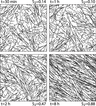
Figure 6. 2D snapshots. Snapshots of configurations of a 2D system evolving over time from an initially empty state. Default parameters.

FIGURE 7

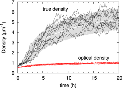
Figure 7. Time evolution of microtubule density. The gray zone indicates the actual microtubule density over time of the 10–90% interval of n = 1000 independent runs, with the average density indicated in white. Black traces show the densities recorded in 10 individual runs. Below, in red, are the optical densities of the same ten runs (a similar band in pink indicates the group statistics, but the band is so narrow that it is hardly visible). Default parameters.

Looking at the time evolution of the degree of alignment as measured by the scalar order parameter S₂ (Figure 8), we see that it saturates long before the density reaches it stationary value. The time-scale of the build-up of the alignment, over the first few hours, is slightly slower than the experimental measurements in Lindeboom et al. [30]. There we showed that microtubule bound nucleation can account for the final factor ≈2 speedup needed to match the biological data. Note, also, that the run-to-run fluctuations in the degree of order are significantly smaller than those of the density. In the following sections we will consider the state at t = 20 h to be representative of the system's steady state alignment.

FIGURE 8

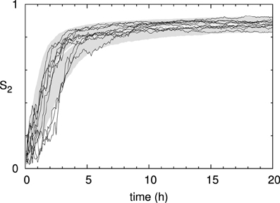
Figure 8. Time evolution of microtubule alignment. S₂ order parameter of the same 1000 runs as in Figure 7. The black curves show the results for 10 individual runs.

5.2. Cross-Validation of Theory and Simulations in the Weak-Interaction Limit

The theory of Hawkins et al. [12] that led to the identification of the control parameter G and the predictions for the bifurcation point G* is based on a mean-field assumption that couples the rates of interaction with densities of microtubules, which specifically neglects both spatial and temporal correlations between subsequent collision events. To validate the correspondence between the theory and simulations, we should therefore choose our interaction parameters such that we are in the limit of a very low frequency of interactions, which effectively decouples subsequent events involving the same microtubule. To probe the low interaction frequency limit we employ the scaling parameter α ≤ 1 introduced in Hawkins et al. [12], which uniformly scales the probabilities of zippering and induced catastrophes from the nominal values shown in Figure 2 and thereby increases the probability of cross-overs.

Moreover, the concept of microtubule bundles is also at odds with the mean-field approximation, because bundles consist of strongly correlated microtubules by definition. In the weak interaction limit we adopt a modified bundle collision model which treats a collision with a bundle of N microtubules as the collision with a single microtubule with an N-times larger probability of zippering or induced catastrophe (maximized at 1). One can show that this is the correct low collision frequency limit of a scheme in which an incoming microtubule can repeatedly collide with all N microtubules separately [18].

As explained in Hawkins et al. [12], the critical control parameter behaves as G*(α) = α^1/3G*(1) under this scaling. In Figure 9 we therefore show the value of the S₂ order parameter as a function of G_c/α^1/3. The results for four values of α show that indeed as α ↓ 0 the onset of the ordering transition appears to converge to the theoretically predicted value G*(1) ≈ −0.15. Previously, we have shown that in the absence of zippering as a source of orientational correlations, the theory can quantitatively describe the simulation data as is [11]. Taken together, these results provide a solid cross-validation of the theory and the simulations in this limit.

FIGURE 9

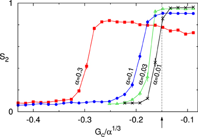
Figure 9. Cross validation of theory and simulations. Order parameter S₂ as a function of the scaled control parameter G_c/α^1/3 for decreasing values of the interaction strength parameter α : 0.3, 0.1, 0.03, 0.01. The arrow and dashed line denote the location of the predicted critical value of the control parameter G*/α^1/3 ≈ −0.15. All data points are averages of n independent runs, and standard errors of the mean are indicated. For α = 0.3, 0.1 we used n = 100 and S₂ was computed at t = 20 h. For α = 0.03, 0.01 a larger equilibration time of t = 100 h was used, and n = 42. Default parameters were used, except for disabling of treadmilling.

5.3. Tubulin Pool

We now consider a system for which the value of the spontaneous catastrophe rate is r_c = 0.0025 s⁻¹. For this low value we find G⁽⁰⁾_c ≈ 0.024, indicating that the microtubules are in the unbounded growth regime (G_c > 0). However, at the same time we limit the available tubulin pool by setting the available tubulin-length density to ρ_tub = 10μm/μm². As Figure 10 shows, the system over time “eats up” the available tubulin, causing the growth speed to decrease in accordance with Eq. (1), and hence also decreasing the effective value of G_c. This process continues until it robustly reaches a steady state for an effective value G^(∞)_c < 0, and the corresponding S₂ value lies on the universal steady state S₂–G_c curve for the default interaction parameters.

FIGURE 10

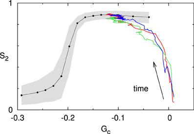
Figure 10. Finite tubulin pool. The colored traces show three independent runs initiated in the unbounded growth regime (G_c > 0; with r_c = 0.0025s⁻¹). Note that all three runs converge to the steady state G_c–S₂ curve computed for these interaction parameters (black line). The gray area denotes the 10–90% range for a set of n = 500 simulations at t = 20h.

5.4. The Importance of Induced Catastrophes, Zippering, and Treadmilling

In this section we empirically probe the effects of three features that intuitively have the potential to influence microtubule alignment. Zippering causes the growing plus ends of microtubules to align with existing microtubules; induced catastrophes punish microtubules that are misaligned with a dominant orientation; treadmilling (especially in combination with zippering) allows dangling minus ends to be removed without the need for the entire microtubule to disappear.

For each permutation of these three features we have performed a series of simulations, spanning a range of values of the G_c parameter. The results are summarized in four panels in Figure 11: the column indicates the presence of induced catastrophes (left: without; right: with) and the row the presence of zippering (top: without; bottom: with). Furthermore, each panel contains curves for systems with and without minus end treadmilling.

FIGURE 11

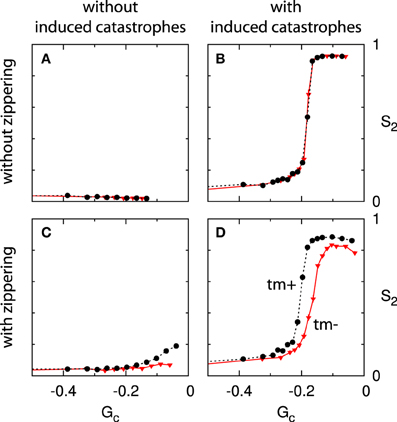
Figure 11. Effect of zippering, induced catastrophes and treadmilling on alignment. Each panels (A–D) shows two G_c−S₂ curves, comparing systems with (tm+; dashed black line) and without (tm-; solid red line) minus end treadmilling. Comparisons between adjacent panels illustrate the effect of induced catastrophes (columns) and zippering (rows). The simulations for non-interacting microtubules (A) were not performed for values of G_c very close to 0 due to diverging numbers of microtubule trajectories. Because alignment cannot occur in the absence of interactions this limitation is not significant. All points are the average of n = 50 independent runs, evaluated at t = 20 h. Standard errors of the mean are shown, but smaller than the data markers for most cases.

These results show that induced catastrophes that suppress discordant microtubules are the main driver of alignment. Zippering alone, on the other hand, is not sufficient to cause significant global alignment, even for high values of G_c (long microtubules). These qualitative results are in agreement with the mean field theory developed in Hawkins et al. [12].

The case of zippering without induced catastrophes (panel C) warrants further discussion. A closer inspection of very dense systems for these parameters reveals that these systems are not aligned (as measured by S₂), but not disordered either. These systems consist of overlapping sets of dense microtubule bundles with dominant angles that differ by more than 40°. This can be understood as follows: microtubules with similar orientations form bundles through zippering interactions. However, in the absence of induced catastrophes, microtubules with orientations that differ by more than 40° can cross each other without impediment, and are free to form bundles with other microtubules having a similar orientation. The result is a system in which independent populations of parallel bundles can coexist. For a zippering angle of 40°, up to four such populations may be present, as 4 × 40° < 180°. The lack of interactions between populations means there is no mechanism for a single orientation to prevail, and this is borne out by simulations with very long run times (see Supplementary Material section 5 for a snapshot of a system at t = 1000 h).

The absence of alignment in Figure 11C is at odds with the results reported in Allard et al. [9] and Eren et al. [10]. In the case of Eren et al. [10], we note that non-isotropic boundary conditions were present for all cases considered. In a sufficiently small system these are able to create net alignment even in the absence of microtubule interactions. In addition, the entropy metric used in that work to quantify the degree of alignment is also sensitive to patterns other than simple alignment, such as the cross-hatch pattern described above. In the work of Allard et al. [9] the interactions between microtubules were detected using a fixed time step, during which a growing plus end traverses approximately 1% of the system size. It is not mentioned how collisions with bundles or multiple collisions within a single time step are processed, which complicates a direct comparison. Furthermore, the small system size of 10 × 10μm enhances any finite-size effects.

Finally, we consider the effect of treadmilling by comparing the curves within each panel of Figure 11. In the absence of zippering (top row), we find that the effect of treadmilling is fully accounted for by the definition of G_c (see also Deinum et al. [17]). In the presence of zippering (bottom row) the additional presence of treadmilling leads to a slight increase in alignment for a given value of G_c. This is consistent with the interpretation that treadmilling removes the discordant dangling ends that remain after zippering. The relative positioning of the curves in panels B and D is dependent on the shape of the angle-dependent interaction function (see Figure 2), but we have consistently observed the relative effect of treadmilling across different interaction functions (data not shown).

Summarizing, we conclude that induced catastrophes are a necessary ingredient for alignment, and zippering alone is not sufficient to establish a dominant orientation. Furthermore, in the presence of zippering and induced catastrophes, treadmilling further enhances alignment (for a given value of G_c).

5.5. Effect of Cell Geometry and Local Changes in Microtubule Dynamics on Array Orientation

The previous sections have focused on the ability of microtubules to form an array, as measured by the alignment order parameter S₂ or its generalization R₂. In this section we consider the orientation of the array as measured by the order parameter Θ₂. Cells within a single type of tissue often show a similar degree of alignment and orientation of their cortical array [31], which indicates that the process of array formation is robust and repeatable. On the other hand, external triggers such as light [2], hormones [32], and mechanical cues [33, 34] are able to modify the array orientation, illustrating that the process is susceptible to orientational cues, which may in turn be subject to cellular control. In this section we investigate factors that affect the orientation of the cortical array. See Figure 12 for an illustration of a longitudinal and a transverse pattern and the associated (R₂, Θ₂) pairs.

FIGURE 12

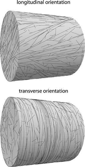
Figure 12. Examples of oriented alignment on cylindrical domains. Top: longitudinal orientation (R₂ = 0.63; Θ₂ = 70°), default parameters at t = 20h. Bottom: transverse orientation (R₂ = 0.88; Θ₂ = 7°). Simulation parameters as on top, except spontaneous catastrophe rate on cylinder caps that have been increased by a factor 2, resulting in reliable transverse ordering.

We consider cylindrical cells with default length L = 40μm and diameter D = 40μm. This cell geometry and size resembles young tobacco BY-2 cells, a commonly used cell line in the investigation of cortical microtubule dynamics. We established a baseline for alignment and orientation by performing 500 runs on this geometry with our default parameter set. The distribution of the resulting order parameters in Figure 13A shows that the systems were generally aligned and favored transverse and longitudinal over intermediate orientations. The geometry does not strongly impose a single orientation, which may be considered a desirable property as it leaves room for regulation by the cell.

FIGURE 13

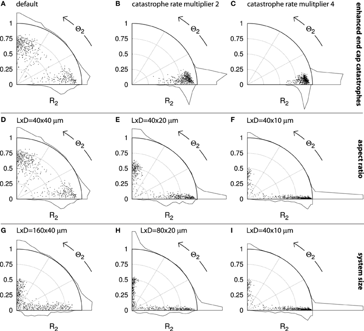
Figure 13. Alignment and orientation in capped cylinder geometries. Each panel contains points that indicate the alignment (S₂) and orientation (Θ₂) of n = 500 independent runs. Histograms for each axis indicate the aggregate distributions. A dot on the horizontal axis represents a perfectly transverse array orientation and a dot on the vertical axis represents a perfectly longitudinal orientation. The further the dot is away from the origin, the stronger the degree of alignment. For cylinders with aspect ratios other than 1 : 1, the maximum attainable R₂ value is angle-dependent (see section 4.2.5). The default cylinder has length L = 40μm and diameter D = 40μm. Simulations were performed using default parameters and the results were analyzed at t = 20h. (A–C): Sequence with increasing multipliers for the spontaneous catastrophe rates on the cylinder end caps: 1 ((A); default), 2 (B), and 4 (C). D–F: Sequence of different aspect ratios, obtained by decreasing the cylinder diameter: D = 40, 20, 10μm, respectively. G–I: Sequence of decreasing absolute system sizes: (L, D) = (160, 40); (80, 20); (40, 10)μm, respectively.

5.5.1. Local changes in microtubule dynamics

One mechanism for cellular control was proposed by Ambrose et al. [35]: a combination of differential crossing probabilities for the different cell edges, resulting from differences in the edges' curvature and the differential presence of (CLASP) proteins that could facilitate edge crossing. The authors performed proof-of-principle simulations for this mechanism and the statistical reliability of this mechanism was further investigated in Deinum [36].

Alternatively, whole regions of the cell could be more or less favorable to microtubule propagation and alignment. Such a cell face-based mechanism has recently been proposed by Vineyard et al. [32] to explain drug-induced array reorientation in A. thaliana hypocotyl cells. We therefore investigated how locally changing the microtubule dynamic instability parameters affects array orientation. We chose to increase the spontaneous catastrophe rate r_c on the end caps, thus effectively making it harder for microtubules to grow longer and interact on these cell faces. Raising the spontaneous catastrophe rate by a factor 2 was sufficient to cause each of the 500 independent simulations in Figure 13B to end with a transverse orientation. Further increasing r_c on the end caps to four times the value on the cylinder body continued this trend and further increased the average degree of alignment (R₂) (Figure 13C).

We note that with the parameters used in Figure 13B the local value of the control parameter G_c on the cylinder caps drops below that of the bulk ordering transition, which occurs for values of r_c between 0.00575 s⁻¹ and 0.0065 s⁻¹. We hypothesize that the local crossing of the ordering transition is the main driving force behind the strong orienting effect of this mechanism. Using r_c = 0.003 s⁻¹ instead of r_c = 0.0045 s⁻¹ (default) on the cylinder wall the end caps remain within the ordered regime, which caused some runs to end with a longitudinal or oblique orientation. Nevertheless, also in that case the vast majority of the runs ended with a transverse orientation (> 80% with Θ₂ < 27°; data not shown). These results demonstrate that subtle orientational cues can be sufficient to establish a strong bias in the cortical array orientation.

5.5.2. Geometric effects

We proceed to dicuss in more detail the role of the cell geometry in determining the cortical array orientation. Increasing the cell's L:D aspect ratio by decreasing the cell's diameter (Figures 13D–F) also caused a shift toward predominantly transversely oriented arrays. In Figure 13F, 84% of all runs have Θ₂ < 27° and 78% have Θ₂ < 4.5°. In this case the intrinsic microtubule dynamics were the same everywhere on the cell's surface and any bias in the preferred orientation must have been a direct effect of the geometry itself. The bias appears to have resulted from finite-size effects.

In support of this interpretation, we found that increasing the absolute size of the elongated cells, whilst keeping the aspect ratio fixed (Figures 13I–G) resulted in a loss of this transverse bias. This result shows that the effects of cell geometry must be considered in relation to the intrinsic length scales l₀ and l of the system (see section 4.1). It is intuitively clear that in an infinitely large system one would encounter locally aligned domains that compete for global dominance. These domains would have certain typical dimensions that would depend on the length scales l₀ and l and possibly on the equilibration time t. Shrinking this hypothetical cell back to more natural proportions, there will be some size at which a single aligned domain is able to “wrap around” the whole cell, thus enabling coordinated alignment over the whole cell surface. This could explain the larger fraction of runs with relatively low R₂ values seen in Figure 13G as compared to Figure 13I and, to a lesser extent, Figure 13H. Natural BY-2 cells and our simulated equivalents in Figure 12 are in this “small cell” regime. Depending on their parameters and geometry, some plant cells may (occasionally) be in the “large cell” regime, as distinct orientational domains within a single cell face have indeed been observed experimentally [37]. We have repeatedly observed the formation of such local domains in our simulations (Deinum [36] and unpublished results), including in systems of realistic sizes.

We repeated the simulations shown in Figure 13 with r_c = 0.0030 s⁻¹ and r_c = 0.0055 s⁻¹ on the cylinder wall (data not shown). As a general trend, we observed that systems that are less entrenched in the ordered parameter regime (i.e., with larger r_c) tended to be more sensitive to subtle orienting effects of the geometry. This is consistent with the idea that close to critical points, where correlations lengths diverge, systems generically become more sensitive to boundary conditions [see e.g., Privman 38].

6. Discussion

We have provided the reader with an overview of the techniques we have developed to study the dynamics and organization of the plant cortical array. As modeling is becoming increasingly central to (cell)biological research (see e.g., [39]), it is only fitting that more attention is devoted to the necessary methodologies. Biological systems are in general highly complex, involving many interacting components giving rise to structures and processes on a wide range of length- and time scales. We believe that the type of event-driven approach presented here is a highly effective tool in enabling the simulation of such systems in a reasonable time frame, as has also been recognized elsewhere [40]. At the same time, we emphasize the utility of complementary analyses using more analytical theoretical approaches. The latter can provide valuable controls on simulations in the form of explicit predictions on limiting cases and expected trends. Moreover, as our use of the control parameter G_c illustrates, results from theory can help to guide parameter choices and thereby significantly reduce the number of simulations required.

In addition to the core biological features described in section 2 and analyzed in section 5, there are further mechanisms that are—out of necessity—beyond the scope of this paper. The two most important of these, both included in our software, are as follows. First, although only briefly mentioned in the text and described in somewhat more detail in the Supplementary Material (sections 2 and 3), our simulation approach can readily incorporate the effects of microtubule severing by the enzyme katanin. A spate of recent articles [2, 41, 42] has underscored the fact that, in concert with adaptor proteins such as SPIRAL2, katanin induced severing is major factor in shaping the ability of the cortical array to change its orientation [2, 34]. We therefore expect this ability to play an important role in future work in this area. Second is the fact that microtubule nucleations are most often initiated from protein complexes bound to pre-existing microtubules and display distinct orientational patterns with respect to the parent microtubule. We have addressed the basic effects of this fact in a previous publication [17]. Work of Lindeboom et al. [2], moreover, shows that the regulation of this mode of nucleation can also play a key role in reorientation processes within the cortical array. We expect that a comprehensive and quantitative approach to modeling, made possible by computational tools such as the one described here, will play a major role in providing a mechanistic understanding of these phenomena.

Data Sharing

The C++ code for the simulations described is available from the authors upon request.

Funding

Simon H. Tindemans was supported by the Computational Life Science programme of NWO. Eva E. Deinum was funded by the Netherlands Consortium for Systems Biology (NCSB). This work is part of the research program of the “Stichting voor Fundamenteel Onderzoek der Materie (FOM),” which is financially supported by the “Nederlandse Organisatie voor Wetenschappelijk Onderzoek (NWO).”

Conflict of Interest Statement

The authors declare that the research was conducted in the absence of any commercial or financial relationships that could be construed as a potential conflict of interest.

Acknowledgments

During the course of this work we have benefitted from discussions with David Ehrhardt, Rhoda Hawkins, Kostya Shundyak, Jan Vos, and Anne Mie Emons. We acknowledge the reviewers for their constructive comments.

Supplementary Material

The Supplementary Material for this article can be found online at: http://www.frontiersin.org/journal/10.3389/fphy.2014.00019/abstract

References

1. Green PB. Mechanism for plant cellular morphogenesis. Science (1962) 138:1404–5. doi: 10.1126/science.138.3548.1404

Pubmed Abstract | Pubmed Full Text | CrossRef Full Text

2. Lindeboom JJ, Nakamura M, Hibbel A, Shundyak K, Gutierrez R, Ketelaar T, et al. A mechanism for reorientation of cortical microtubule arrays driven by microtubule severing. Science (2013) 342:1245533. doi: 10.1126/science.1245533

Pubmed Abstract | Pubmed Full Text | CrossRef Full Text

3. Baskin TI. On the alignment of cellulose microfibrils by cortical microtubules: a review and a model. Protoplasma (2001) 215:150–71. doi: 10.1007/BF01280311

Pubmed Abstract | Pubmed Full Text | CrossRef Full Text

4. Gutierrez R, Lindeboom JJ, Paredez AR, Emons AMC, Ehrhardt DW. Arabidopsis cortical microtubules position cellulose synthase delivery to the plasma membrane and interact with cellulose synthase trafficking compartments. Nat Cell Biol (2009) 11:797–806. doi: 10.1038/ncb1886

Pubmed Abstract | Pubmed Full Text | CrossRef Full Text

5. Paredez AR, Somerville CR, Ehrhardt DW. Visualization of cellulose synthase demonstrates functional association with microtubules. Science (2006) 312:1491–5. doi: 10.1126/science.1126551

Pubmed Abstract | Pubmed Full Text | CrossRef Full Text

6. Shaw SL, Kamyar R, Ehrhardt DW. Sustained microtubule treadmilling in arabidopsis cortical arrays. Science (2003) 300:1715–8. doi: 10.1126/science.1083529

Pubmed Abstract | Pubmed Full Text | CrossRef Full Text

7. Dixit R, Cyr R. Encounters between dynamic cortical microtubules promote ordering of the cortical array through angle-dependent modifications of microtubule behavior. Plant Cell (2004) 16:3274–84. doi: 10.1105/tpc.104.026930

Pubmed Abstract | Pubmed Full Text | CrossRef Full Text

8. Baulin VA, Marques CM, Thalmann F. Collision induced spatial organization of microtubules. Biophys Chem (2007) 128:231–44. doi: 10.1016/j.bpc.2007.04.009

Pubmed Abstract | Pubmed Full Text | CrossRef Full Text

9. Allard JF, Wasteneys GO, Cytrynbaum EN. Mechanisms of self-organization of cortical microtubules in plants revealed by computational simulations. Mol Biol Cell (2010) 21:278–86. doi: 10.1091/mbc.E09-07-0579

Pubmed Abstract | Pubmed Full Text | CrossRef Full Text

10. Eren EC, Dixit R, Gautam N. A three-dimensional computer simulation model reveals the mechanisms for self-organization of plant cortical microtubules into oblique arrays. Mol Biol cell (2010) 21:2674–84. doi: 10.1091/mbc.E10-02-0136

Pubmed Abstract | Pubmed Full Text | CrossRef Full Text

11. Tindemans SH, Hawkins RJ, Mulder BM. Survival of the aligned: ordering of the plant cortical microtubule array. Phys Rev Lett (2010) 104:058103. doi: 10.1103/PhysRevLett.104.058103

Pubmed Abstract | Pubmed Full Text | CrossRef Full Text

12. Hawkins R, Tindemans S, Mulder B. Model for the orientational ordering of the plant microtubule cortical array. Phys Rev E (2010) 82:011911. doi: 10.1103/PhysRevE.82.011911

Pubmed Abstract | Pubmed Full Text | CrossRef Full Text

13. Eren EC, Gautam N, Dixit R. Computer simulation and mathematical models of the noncentrosomal plant cortical microtubule cytoskeleton. Cytoskeleton (2012) 69:144–54. doi: 10.1002/cm.21009

Pubmed Abstract | Pubmed Full Text | CrossRef Full Text

14. Deinum EE, Mulder BM. Modelling the role of microtubules in plant cell morphology. Curr Opin Plant Biol (2013) 16:688–92. doi: 10.1016/j.pbi.2013.10.001

Pubmed Abstract | Pubmed Full Text | CrossRef Full Text

15. Dogterom M, Leibler S. Physical aspects of the growth and regulation of microtubule structures. Phys Rev Lett (1993) 70:1347–50. doi: 10.1103/PhysRevLett.70.1347

Pubmed Abstract | Pubmed Full Text | CrossRef Full Text

16. Nakamura M, Ehrhardt DW, Hashimoto T. Microtubule and katanin-dependent dynamics of microtubule nucleation complexes in the acentrosomal Arabidopsis cortical array. Nat Cell Biol (2010) 12:1064–70. doi: 10.1038/ncb2110

Pubmed Abstract | Pubmed Full Text | CrossRef Full Text

17. Deinum EE, Tindemans SH, Mulder BM. Taking directions: the role of microtubule-bound nucleation in the self-organization of the plant cortical array. Phys Biol (2011) 8:056002. doi: 10.1088/1478-3975/8/5/056002

Pubmed Abstract | Pubmed Full Text | CrossRef Full Text

18. Tindemans SH. Biomolecular Design Elements : Cortical Microtubules and DNA-Coated Colloids. Wageningen, NL: Wageningen University (2009)

19. Mitchison T, Kirschner M. Dynamic instability of microtubule growth. Nature (1984) 312:237–42. doi: 10.1038/312237a0

Pubmed Abstract | Pubmed Full Text | CrossRef Full Text

20. Lagomarsino MC, Tanase C, Vos JW, Emons AMC, Mulder BM, Dogterom M. Microtubule organization in three-dimensional confined geometries: evaluating the role of elasticity through a combined in vitro and modeling approach. Biophys J (2007) 92:1046–57. doi: 10.1529/biophysj.105.076893

Pubmed Abstract | Pubmed Full Text | CrossRef Full Text

21. Vos JW, Dogterom M, Emons AMC. Microtubules become more dynamic but not shorter during preprophase band formation: a possible “search-and-capture” mechanism for microtubule translocation. Cell Motil Cytoskeleton (2004) 57:246–58. doi: 10.1002/cm.10169

Pubmed Abstract | Pubmed Full Text | CrossRef Full Text

22. Sainsbury F, Collings DA, Mackun K, Gardiner J, Harper JDI, Marc J. Developmental reorientation of transverse cortical microtubules to longitudinal directions: a role for actomyosin-based streaming and partial microtubule-membrane detachment. Plant J (2008) 56:116–31. doi: 10.1111/j.1365-313X.2008.03574.x

Pubmed Abstract | Pubmed Full Text | CrossRef Full Text

23. Gardiner JC, Harper JD, Weerakoon ND, Collings DA, Ritchie S, Gilroy S, et al. A 90-kD phospholipase D from tobacco binds to microtubules and the plasma membrane. Plant Cell (2001) 13:2143–58. doi: 10.2307/3871433

Pubmed Abstract | Pubmed Full Text | CrossRef Full Text

24. Kirik V, Herrmann U, Parupalli C, Sedbrook JC, Ehrhardt DW, Hülskamp M. CLASP localizes in two discrete patterns on cortical microtubules and is required for cell morphogenesis and cell division in Arabidopsis. J Cell Sci (2007) 120:4416–25. doi: 10.1242/jcs.024950

Pubmed Abstract | Pubmed Full Text | CrossRef Full Text

25. Barton DA, Vantard M, Overall RL. Analysis of cortical arrays from Tradescantia virginiana at high resolution reveals discrete microtubule subpopulations and demonstrates that confocal images of arrays can be misleading. Plant Cell (2008) 20:982–94. doi: 10.1105/tpc.108.058503

Pubmed Abstract | Pubmed Full Text | CrossRef Full Text

26. Do Carmo MP. Differential Geometry of Curves and Surfaces. Englewood Cliffs, NJ: Prentice-Hall (1976).

27. Fichthorn KA, Weinberg WH. Theoretical foundations of dynamical Monte Carlo simulations. J Chem Phys (1991) 95:1090. doi: 10.1063/1.461138

CrossRef Full Text

28. Lucas J, Shaw SL. Cortical microtubule arrays in the Arabidopsis seedling. Curr Opin Plant Biol (2008) 11:94–8. doi: 10.1016/j.pbi.2007.12.001

Pubmed Abstract | Pubmed Full Text | CrossRef Full Text

29. Gramsbergen E, Longa L, De Jeu WH. Landau theory of the nematic-isotropic phase transition. Phys Rep (1986) 135:195–257. doi: 10.1016/0370-1573(86)90007-4

CrossRef Full Text

30. Lindeboom JJ, Lioutas A, Deinum EE, Tindemans SH, Ehrhardt DW, Emons AMC, et al. Cortical microtubule arrays are initiated from a nonrandom prepattern driven by atypical microtubule initiation. Plant Physiol (2013) 161:1189–201. doi: 10.1104/pp.112.204057

Pubmed Abstract | Pubmed Full Text | CrossRef Full Text

31. Lloyd CW. Plant Microtubules: Their Role in Growth and Development. New York, NY: John Wiley & Sons, Ltd (2001). doi: 10.1002/9780470015902.a0001685.p

CrossRef Full Text

32. Vineyard L, Elliott A, Dhingra S, Lucas JR, Shaw SL. Progressive transverse microtubule array organization in hormone-induced Arabidopsis hypocotyl cells. Plant Cell (2013) 25:662–76. doi: 10.1105/tpc.112.107326

Pubmed Abstract | Pubmed Full Text | CrossRef Full Text

33. Hamant O, Heisler MG, Jönsson H, Krupinski P, Uyttewaal M, Bokov P, et al. Developmental patterning by mechanical signals in Arabidopsis. Science (2008) 322:1650–5. doi: 10.1126/science.1165594

Pubmed Abstract | Pubmed Full Text | CrossRef Full Text

34. Uyttewaal M, Burian A, Alim K, Landrein B, Borowska-Wykręt D, Dedieu A, et al. Mechanical stress acts via katanin to amplify differences in growth rate between adjacent cells in Arabidopsis. Cell (2012) 149:439–51. doi: 10.1016/j.cell.2012.02.048

Pubmed Abstract | Pubmed Full Text | CrossRef Full Text

35. Ambrose C, Allard JF, Cytrynbaum EN, Wasteneys GO. A CLASP-modulated cell edge barrier mechanism drives cell-wide cortical microtubule organization in Arabidopsis. Nat Commun (2011) 2:430. doi: 10.1038/ncomms1444

Pubmed Abstract | Pubmed Full Text | CrossRef Full Text

36. Deinum EE. Simple Models for Complex Questions on Plant Development. Wageningen: Wageningen University (2013).

37. Chan J, Calder G, Fox S, Lloyd C. Cortical microtubule arrays undergo rotary movements in Arabidopsis hypocotyl epidermal cells. Nat Cell Biol (2007) 9:171–5. doi: 10.1038/ncb1533

Pubmed Abstract | Pubmed Full Text | CrossRef Full Text

38. Privman V. Finite Size Scaling and Numerical Simulation of Statistical Systems. Singapore: World Scientific Pub Co Inc (1990).

39. Mogilner A, Allard J, Wollman R. Cell polarity: quantitative modeling as a tool in cell biology. Science (2012) 336:175–79. doi: 10.1126/science.1216380

Pubmed Abstract | Pubmed Full Text | CrossRef Full Text

40. van Zon JS, ten Wolde PR. Green's-function reaction dynamics: a particle-based approach for simulating biochemical networks in time and space. J Chem Phys (2005) 123:234910. doi: 10.1063/1.2137716

Pubmed Abstract | Pubmed Full Text | CrossRef Full Text

41. Wightman R, Chomicki G, Kumar M, Carr P, Turner SR. SPIRAL2 determines plant microtubule organization by modulating microtubule severing. Curr Biol (2013) 23:1902–7. doi: 10.1016/j.cub.2013.07.061

Pubmed Abstract | Pubmed Full Text | CrossRef Full Text

42. Zhang Q, Fishel E, Bertroche T, Dixit R. Microtubule severing at crossover sites by Katanin generates ordered cortical microtubule arrays in arabidopsis. Curr Biol (2013) 23:2191–5. doi: 10.1016/j.cub.2013.09.018

Pubmed Abstract | Pubmed Full Text | CrossRef Full Text