Statistical analysis of protein ensembles

1. Introduction

The comparison of proteins and other chemicals in general is a relevant topic in many scientific fields. Perhaps one of the most important applications is drug design [1]. Its importance is also signaled by the many existing approaches and similarity measures elaborated in the last decades (see the review of Nikolova and Jaworska 2).

The literature of the comparison methods is vast and we do not intend to list and overview all the techniques that have been developed to tackle these problems. However, we would like to enumerate a few approaches in order to motivate the present work.

First of all, the comparison methods can be divided into two broad classes: superposition and descriptor methods [3]. The former aim to calculate the best alignment of the molecules and quantify the similarities as some measure of the overlap while methods in the latter category describe the molecules with certain feature vectors and assess similarities by comparing the features, thus being independent from molecular orientation. Most methods in both categories treat molecules as rigid objects, however, in the last decade plenty of methods emerged which address flexibility, too.

Aligners first choose a scoring function which indicates the overlap of the compared molecules. Once the choice is made, the correspondence among molecules has to be found, which is an optimization problem. Thus, the crucial step here is the choice of the scoring function. Although there are few empirically parameterized models, the methods are based on “ad hoc” scoring functions [4]. Flexibility is usually treated in the mechanical sense, aligners define rigid substructures but allow movements at the joints of these [4].

Descriptor based methods seek to build a rotation and translation invariant signature to represent a molecule and use the signature to compare these molecules [5]. However, similarly to the scoring functions of the aligners, these signatures are mostly based on heuristic algorithms and they seldom have a rigorous mathematical motivation. Perhaps the methods with the most theoretical foundations are the ones based on graph theory [6]. Additionally, descriptors come short to deal with flexible molecules as addressing this issue in terms of signatures is still challenging [5].

Although, as noted above, many approaches exist, it is evident that they often lack mathematical rigor, especially when treating flexible molecules, despite the fact that a solid mathematical basis is required in order to ensure reliability. While methods, such as the ones relying on geometric comparison of molecules, may fail when handling flexible structures, these approaches possess a proper theoretical foundation. Geometric comparison methods, for instance, are usually based on volume overlaps, i.e., set intersections in a mathematical terminology, and they perform extremely well on rigid bodies. To achieve a similar performance for flexible structures, it is indispensable to base the approaches on mathematics specifically developed for studying flexible manifolds, namely mathematical topology. Proper mathematical handling should be, of course, only the basis on which methods should build the knowledge from chemistry, physics and biology. This is especially the case since in recent years flexibility turned out to be a very important feature of many proteins [7] as it may influence binding affinity [8] and functionality [9]. We believe, it is crucial to minimize possible flaws and place methods addressing the comparison of flexible molecules in a proper mathematical context.

We approach the problem of comparing flexible structures from this perspective. We introduce a framework, relying mainly on elements of computational topology and graph theory. The framework is intended to support a basic comparison method relying on the calculation of certain topological properties of the molecules, in terms of topological invariants, on different geometric scales. A given configuration of a protein is a representation of a topological space which is homeomorphic with all the possible foldings of the chemical structure. Based on this, we elaborate a method, enabling a comparison which takes into account the possibly flexible nature of certain molecules. We do this without considering chemical information.

We emphasize that we do not intend to provide yet another ready-to-use method for classifying/scoring proteins which would outperform the existing ones. In turn, we would like to introduce a framework which allows the elaboration of new, possibly different comparison methods. The proposed approach is not an aligner, therefore comparing it to existing protein aligners is not reasonable. On the other hand, while the framework can be perceived as a descriptor, it is much more generic, for instance, it allows the calculation of other properties (e.g., compressibility 10). While descriptors highlight different features of proteins, the here introduced approach is very versatile and the used topological representation may encode different descriptors in different ways.

Of course, we understand that the field needs approaches which, based on recorded crystallographic configurations, are able to infer different properties of proteins. We strongly believe that the ideas presented in this paper may open the path to fruitful approaches through the application of computational topology.

One of the huge benefits of the framework is its modularity: topological representations may be altered to suit specific needs; different methods may be used to compare topological invariants (see for instance 8, 11); the clustering method used to sort the different proteins based on the calculated measures may also be changed. All these modifications can be carried out independently from each other. Possibilities are numerous and surveying all of them is out of the scope of this paper. In addition, knowledge as chemical information can constitute an “extra dimension” of the analysis and can be taken into account in different ways.

We demonstrate that the framework is viable by finding the correspondence between different foldings of the same proteins. In this sense, the presented application is not a classical protein classification, but rather a simple proof of principle.

2. Methods

2.1. Topological Invariants

Our method relies on the calculation of the persistence intervals of the Betti numbers [12] for the investigated structures. Betti numbers [13] are the counts of different topological features like connected components (0th Betti number), holes (1st Betti number), voids (second Betti number) and their higher-dimensional generalizations. Of course, since real world structures are three-dimensional ones, we do not have to deal with these generalizations. The persistence intervals of these features denote the geometric scales on which the given features do not change. To have a better understanding of the concept, let us consider the following scenario. Let S = {(x,y,z)| x, y, z ∈ R} be a point-set sample of an unknown O object embedded in the three-dimensional space, where R is the set of real numbers. Note that O could consist of multiple pieces (components). In order to calculate the Betti numbers, that is, count the components, the holes and the voids present in O based on the S sample, we have to reconstruct O from S. One could conceive different ways of reconstructing the object. Perhaps the most straightforward method is to connect each point with its nearest neighbors. We can define the nearest neighbors of the points by calculating the Delaunay triangulation [14] of S and discard the edges which are larger than an l_c cutoff length. This cutoff length can be defined as some fraction of the maximal edge-length in the triangulation, for instance. The remaining triangles are considered face elements and the tetrahedrons are treated as solid volume.

Components are relatively easy to count. Any two points from S which have a path between them along the edges of the triangulation (that is, they are connected) are in the same component. Two points connected by no path are in different components. Components thus can be counted by counting the subsets of S which are not connected to each other through the edges of the triangulation.

Counting holes and voids is a bit more difficult. In order to illustrate the problem, imagine a ball. It has a single component (everything is connected), no holes (otherwise the air would escape) and a single void (the space enclosed by the shell of the ball). A single perforation on the surface of the ball is not considered a hole. The reasoning behind this is the following: in theory, we could hold the ball membrane from the boundaries of the perforation and stretch it out until the membrane flattens out completely. Thus a ball with an opening on a membrane is homeomorphic to a plane without holes. If we puncture the shell again, we will have an object homeomorphic with a plane with a hole on it. Thus only the second hole on the surface of the ball is counted as a hole. Note also that as soon as we created the first perforation, the void disappears because of the homeomorphism with the plane. When counting holes and voids, one has to take into account these effects. For instance, only the triangle-faced polyhedrons with more then four faces create voids.

Considering these criteria, we can proceed with the calculation of the Betti numbers for the object obtained through the reconstruction process based on S. If S is a good sample and is dense enough, that is, the distance between nearest neighbors in S is roughly uniform and is much smaller than the diameter of O, then S captures well the topology of O and the Betti numbers measured on S will be good descriptors of the topology of O.

However, if S is a sparse sample of O, the reconstruction procedure may yield an incorrect representation of O. To render the method more robust, instead of considering only one geometric scale defined by the fixed cutoff-length of the triangle edges, we consider more geometric scales by varying l_c from zero to infinity. We calculate the Betti numbers for each value of l_c and register it. Calculating the Betti numbers infinitely many times is not feasible of course, however, in practice, it is enough to consider the length of the longest edge in the triangulation as the upper bound for l_c. Figure 1 illustrates the process of reconstructing a particular object for different l_c cutoff values.

FIGURE 1

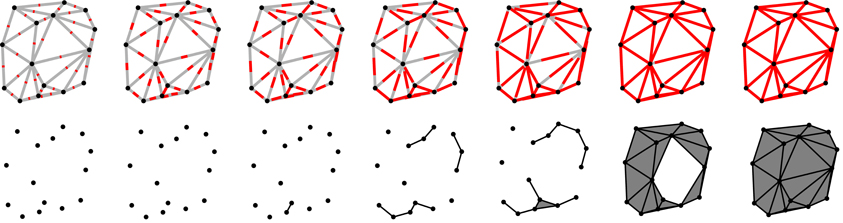
Figure 1. The figure illustrates how a particular point-set is scanned on different scales. The length scale (the cutoff l_c) is indicated by the length of the red lines in the upper row. In the same row, gray lines indicate the edges in the Delaunay triangulation. When the length of the red segments is equal (or larger) to that of a particular edge, it means that the endpoints of that edge are separated by a distance correspondent to the value of the l_c cutoff (or they are closer) and they are connected at this stage. The process of connecting the points is indicated in the lower row. Distances are of course measured from one point to another and not from the middle of the segments, the red lines serve only as a visual indication of the value of the cutoff l_c. Note that when all three edges of a triangle are formed, the triangle itself is also added to the object (these triangles are shaded by a darker gray color in the lower row). In the first two scales (from the left) the cutoff l_c is smaller than any distance between the points, thus no points are connected yet and there are 15 connected component (each point is a separate connected component), and no holes (voids cannot form as the example is in two dimensions). At the third scale (third column from the left), the cutoff exceeds the distance between two of the points and they are connected, thus there will be 14 connected components, the freshly connected pair forming a single connected component. At the fifth scale (fifth column from the left), the first triangle is formed and added to the object. At this stage there are four connected components but still no holes. At the next cutoff level (sixth column from the left), most of the triangles had formed and they enclose a hole (the white unshaded region). In this case we have a single connected component (all the points are connected) and a hole. Note that holes need not be surrounded by formed triangles. Edges also can form holes. In the last column, the cutoff has reached a value larger or equal to that of the longest edge in the triangulation and all the edges and triangles are added to the object, thus the hole observed in the previous column is filled in. In this case the object has a single connected component and no hole.

In principle we could use any triangulation or any (even non-planar) graph defined on the S set. The Delaunay triangulation, however, is a good compromise between calculation complexity and memory efficiency when calculating the Betti numbers. Considering the complete graph on S is, in computational topology terms, equivalent to the construction of the Rips-complex [15], while the Delaunay construction is analogous to the calculation of the α-complex [16].

Given that a hole exists at a particular cutoff l_c, there is a largest cutoff l′_c ≤ l_c, for which the hole is not yet present in the reconstructed object and there is a smallest one l″_c ≥ l_c for which the hole is filled in. The interval (l′_c, l″_c) is the persistence interval of the mentioned hole. The wider the interval, the more important (persistent) the corresponding topological feature is. Although the triangulation may alter even for small coordinate changes, important/persistent features are usually not influenced by such effects if the sampling is good enough. These features are altered only when the structure of the whole point-set is changed.

Betti numbers are topological invariants as their value is invariant under continuous deformation of the objects such as stretching or bending, for instance (tearing and gluing are not continuous deformations). Continuous deformations do not change the topology of the objects, thus Betti numbers are handy invariants when comparing different topologies.

Calculating Betti numbers is generally a relatively abstract and complex task and requires a deeper understanding of algebraic and computational topology. A very sketchy pseudo-code is presented in Algorithm 1. The reader is referred to Edelsbrunner and Harer [13] for details. However, plenty of open source software packages were developed in recent years which enable the calculation of these topological invariants [17–19].

ALGORITHM 1

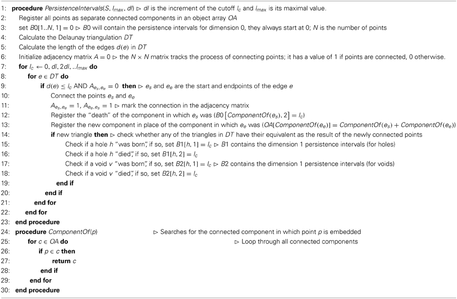
Algorithm 1. Calculating the persistence intervals.

2.2. A Graphical Representation of the Topology

There is a convenient way to represent the information gained through the scanning of S described above. Instead of simply counting the components, holes and voids, we construct a diagram for each of the Betti numbers. The horizontal axis of the diagram will correspond to the l_c cutoff. We represent each instance of components, holes and voids on the corresponding diagram with a horizontal bar. The starting-point of the bar corresponds to the cutoff value at which the instance was created while the end-point of the bar is the cutoff value at which the instance ceased to exist. The vertical ordering of the bars is arbitrary. This representation was developed by Carlsson and his collaborators (see, for instance, Carlsson 12. For a short review see Ghrist 20). In Figure 2 we present such a plot for a particular point-set.

FIGURE 2

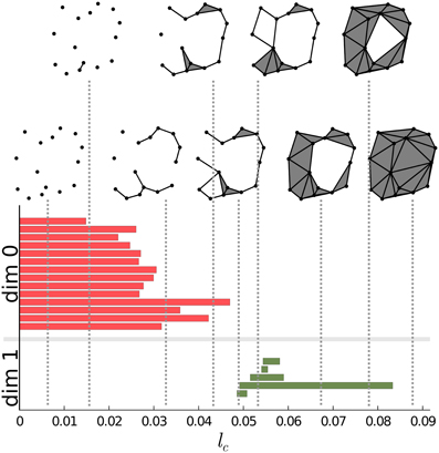
Figure 2. Persistence intervals for a particular set of points. Red bars represent the dimension 0 intervals, green bars represent dimension 1 intervals. Note that for connected components there is an interval which closes at ∞. Since this bar is present for any non-empty point-set, it carries no information, therefore it can be removed from the representation. The process of connecting the points is also presented on the upper side of the figure for certain values of the l_c cutoff.

Carlsson's diagrams can be viewed as a fingerprint, a barcode of the structure. It encodes all the information regarding the Betti numbers on different scales. Betti numbers can be extracted by drawing a vertical line at any cutoff value and counting the numbers of the intersections with the bars of the diagram. Barcodes for components, holes and voids are also called dimension zero, dimension one and dimension two intervals/barcodes, respectively. These barcodes constitute the topological basis of our approach.

Dimension zero intervals are somewhat special. Since all the points exist for l_c = 0, and none of them are connected at this cutoff value, all the points are in different components. There will be as many zero dimension intervals as many points there are and all these intervals will have a starting point of zero. As we increase the l_c cutoff, points will start to be connected. Whenever two points from two different components are connected the components will be unified and the number of components is decreased, thus one of the intervals representing the just connected components is closed. Note that for any nonempty point-set there is always at least one component. Therefore, one of the intervals will always range from zero to infinity. Being always the same, it carries no information, thus it can be removed from the set of intervals.

2.3. The Distribution of Topological Features

Objects, in general, can be characterized by the size of their components, the way these are joined together and the size of the holes and voids that form during the building process. On the other hand, the end-points of the dimension zero bars have values statistically proportional to the spacing between sub-components of the system, while their number carry information regarding the size of the represented structure. The end-points of the dimension one bars have values statistically proportional to the diameters of the holes in the system. Similarly, end-points of the dimension two bars have values statistically proportional to the diameters of the voids. The dimension zero intervals always start at zero, thus it is only the end-point which matters in this case. The starting points of the dimension one and two intervals would mostly depend on the density of the points. In this sense, it is enough to describe the objects with the end-points of the intervals. Even more, we can replace the set of the end-points by the distribution of these, that is, by the normalized sum of Dirac delta functions centered at the end-points of the intervals, thus representing an object with a probability distribution. Then we can measure the similarity/dissimilarity between two objects as the similarity/dissimilarity between the representing distributions.

2.4. The Wasserstein Distance

There are a number of ways to compare two distributions. One can calculate any of the suitable f-divergence measures [21], for instance, the Kullback–Leibler divergence [22]. However, these measures are not necessary proper distances, in particular, they may not be symmetric or transitive. Another approach is to calculate the Wasserstein (or Vasershtein in the original spelling) distance (for a comprehensive review see Villani 23 between the probability densities). The Wasserstein distance is a proper metric and can informally be introduced with a simple analogy: the distance is proportional to the physical work needed to transform a pile of earth shaped like one of the density functions to a pile shaped like the other density function. Based on this analogy, the Wasserstein distance is sometimes referred to as the earth movers distance (EMD). In fact, the Wasserstein distance is a class of distances parameterized with a p ≥ 1 parameter in which the EMD corresponds to the 1st (p = 1) Wasserstein distance. As in the present work we only use the 1st Wasserstein distance, we may drop the notation regarding the parameterization or we will simply refer to it as EMD.

Given two probability density functions f_X and g_Y, a more mathematical definition of the EMD can be given as

$\begin{array}{cc}{d}_{EMD}(f_X,g_Y)=\underset{{\gamma }_{XY}}{\inf }E\left[d(x,y)\right]\text{,}& \left(1\right)\end{array}$

where the infimum is taken over the joint distribution γ_XY of x and y with marginals f_X and g_Y. d(X,Y) is a distance function and in the simplest case is the absolute difference of the arguments, that is, d(X,Y) = |X − Y|.

3. Application and Results

We measure dissimilarity between two chemical structures as indicated in the previous sections. We treat a molecule as a point-set defined by the coordinates of its atoms. We calculate the persistence intervals and compute the distribution of the upper boundaries of the intervals. We proceed in this manner for each molecule we want to classify. Finally we calculate the Wasserstein distance among each pair of distributions, constructing thus a fully connected weighted graph of the molecule ensembles with the weights corresponding to the Wasserstein distances.

In order to classify the molecules, we simply need to cluster the obtained graph. For this purpose we apply the k-means algorithm [24]. This algorithm simply divides the sample into k groups so that the formed groups are as compact as possible.

We used different software to conduct our studies. We calculated the persistence intervals using the Dionysus software [17], we computed the Wasserstein distances with a code provided by the authors of Ref. [25], available for free online on their website. We carried out the clustering step with the built-in k-means algorithm of the MatLab's statistical toolbox, but, of course, any implementation of k-means is suitable. A source code to reproduce the results is available online (http://wwwcp.tphys.uni-heidelberg.de/plos/calculate_clustering.zip).

3.1. The Ensemble Protein Database

For testing and demonstrative purposes, we apply our approach to a set of structures obtained from the Ensemble Protein Database (EPDB) [26]. We analyze five approximate ensembles constructed for the following proteins: Barstar (1A19), Calmodulin (1CFD), Ferredoxin-2 (1FXD), Alpha-Amylase inhibitor (1HOE), and Human CDC25B Catalytic Domain (1QB0). There are 191 configurations for Barstar, 196 for Calmodulin, 141 for Ferrodexin-2, 129 for the Alpha–Amylase inhibitor and 495 for the Human CDC25B Catalytic Domain.

Feeding the configurations to our method, without including any information about the origin of the conformations, we expect that the approach is able to distinguish between the different proteins. We will compare each protein configuration with every other configuration and calculate the Wasserstein distance for all of the pairs. It is convenient to display the results of the comparison in a color-coded matrix where each row and column corresponds to a protein. The ordering of the proteins in the rows and the columns are the same. Throughout the rest of the paper we apply the same ordering of the proteins in each figure, where the first 191 rows/columns represent the Barstar protein, the next 196 represent the Calmodulin, the next 141 contain results for the Ferrodexin-2, the following 129 represent the Alpha–Amylase inhibitor, while the last 495 rows/columns display results for the Human CDC25B Catalytic Domain.

Figure 3 presents the calculated Wasserstein distances for the dimension zero intervals. Looking at the figure, we see that the Wasserstein distances within certain groups are smaller than the inter-group distances and we actually can separate five groupings. In order to give an explicit grouping of the configurations by applying the k-means algorithm, we need to make sure that our guess of requesting k = 5 clusters based on the visual inspection of Figure 3 is indeed a good choice. For this reason, we calculate clusterings for different cluster numbers, letting k run from 1–10. For each k value, we randomly select 10 configurations from the ensembles for each protein and we feed the set of selected configurations to the k-means algorithm. In order to decide whether a clustering is good or not, we calculate the mean distance to the center for each cluster and characterize a clustering with the sum of these means. In mathematical terms, we define this sum as:

$\begin{array}{cc}S(k)={\displaystyle \sum _{i=1}^k{\langle \left|\right|Z_i-c_i\left|\right|\rangle }_Z}\text{,}& \left(2\right)\end{array}$

where Z_i represents the “coordinates” of a protein in the ith cluster with center c_i (c_i = 〈 Z_i 〉_Z) and ‖.‖ is the euclidean norm. The coordinates are in fact the Wasserstein distances to all other proteins, that is, a row in the distance-matrix. We consider a clustering with k clusters good if the S(k) sum is low.

FIGURE 3

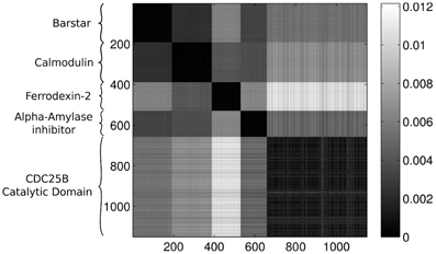
Figure 3. Wasserstein distances for the distributions representing the dimension 0 intervals. Each row and column corresponds to a protein-configuration, the ordering of the rows and the columns are the same. A darker shade means small distance while lighter shades imply larger distances. Note the dark blocks on the diagonal, they correspond to protein-groups which are close to each other.

To avoid problems caused by the probabilistic nature of k-means, we repeat the clustering many times for different samples, thus generating an ensemble of clusterings, and present the results averaged over this ensemble. In other words, the result of the clusterings are presented in a matrix form where each row and column corresponds to a protein and the matrix entry at the intersection of a given row and a given column is the probability of finding the two proteins corresponding to the row and the column in the same cluster, calculated based on the ensemble of the clusterings.

Figure 4 presents the S(k) curve for the clustering of the dimension zero data. As it can be seen, the curve predicts that k = 5 or k = 6 gives us a relatively good clustering. If we look at the actual clusterings (shown for k = 5 in Figure 5 and for k = 6 in Figure 6) based on which S(k) was calculated, we see that the clusterings for k = 5 and k = 6 are in fact equivalent. Setting k to 6 allows more flexibility for the clustering, than the k = 5 case, but it is clear that there are five groups, exactly corresponding to the different proteins. Thus, this clearly indicates, that the method is able to find the original groups.

FIGURE 4

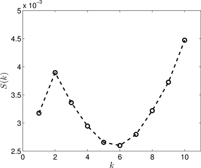
Figure 4. The S(k) curve for the clustering of the dimension 0 data, calculated based on Equation (2).

FIGURE 5

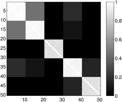
Figure 5. Probability of the event when two proteins are assigned to the same class when k = 5 classes are requested. The probability is calculated for each pair of proteins from different sub-samples of the ensemble. The proteins for a given position in a row/column were selected randomly from the ensemble with the constraint that they always belong to the same group. Probabilities are calculated by repeating the clustering multiple times and counting how many times the pairs were co-classified.

FIGURE 6

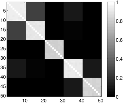
Figure 6. Probability of the event when two proteins are assigned to the same class when k = 6 classes are requested. The probability is calculated for each pair of proteins from different sub-samples of the ensemble. The proteins for a given position in a row/column were selected randomly from the ensemble with the constraint that they always belong to the same group. Probabilities are calculated by repeating the clustering multiple times and counting how many times the pairs were co-classified.

Clustering the entire dataset in five clusters gives the results presented in Figure 7. We can clearly see the five groups of proteins, four smaller strongly coupled groups (corresponding to the proteins 1A19, 1CFD, 1FXD, and 1HOE) and one larger group (corresponding to 1QB0). Members of the last group are not coupled as strongly as the members of the other groups but they always classify in the same way and do not mix with the other proteins. While there is some mixing in the first two and the fourth group, the core groups are clearly distinguishable.

FIGURE 7

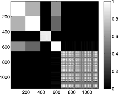
Figure 7. Probability of the event when two proteins are assigned to the same class when k = 5 classes are requested for the dimension 0 data. The probability is calculated for each pair of proteins by repeating the clustering multiple times and counting how many times the pairs were co-classified.

Figure 8 presents the Wasserstein distances for the dimension one intervals. Looking at the figure it is obvious, that the dimension one intervals indicate two groups. Performing the same check as in the case of the dimension zero intervals, we see in Figure 9 that the S(k) measure also indicates that clustering the dataset into two clusters is a good choice in this case.

FIGURE 8

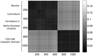
Figure 8. Wasserstein distances for the distributions representing the dimension 1 intervals. Each row and column corresponds to a protein-configuration, the ordering of the rows and the columns are the same. A darker shade means small distance while lighter shades imply larger distances. Note the dark blocks on the diagonal, they correspond to protein-groups which are close to each other.

FIGURE 9

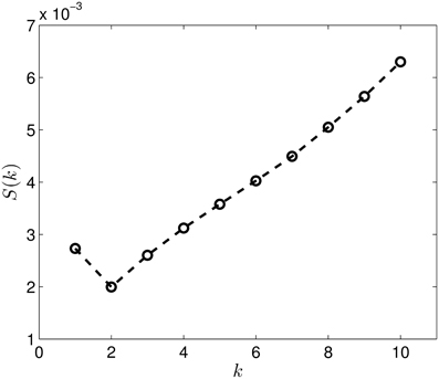
Figure 9. The S(k) curve for the clustering of the dimension 1 data, calculated based on Equation (2).

Performing the clustering for k = 2 we get the results shown in Figure 10, which clearly gives two clusters, putting the first four groups of proteins (1A19, 1CFD, 1FXD, 1HOE) in the same class while the last group (1QB0) forms a different class. The explanation behind this result is that while the proteins corresponding to the first four groups are comparable in size (containing 89, 72, 58, and 74 residues, respectively), the last protein is much larger (177 residues). In fact the mixing of the first two and the fourth group we see in Figure 7 is probably also a size-related effect as these groups are very close to each other in size, while the third group is a bit smaller. Nevertheless, it is now clear that by looking at the dimension one intervals, we in fact classify the proteins with respect to their sizes but we avoid calculating the geometric similarity which is a computationally very expensive procedure, as one needs to calculate the best overlaps among the structures.

FIGURE 10

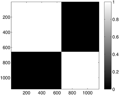
Figure 10. Probability of the event when two proteins are assigned to the same class when k = 2 classes are requested for the dimension 1 data. The probability is calculated for each pair of proteins by repeating the clustering multiple times and counting how many times the pairs were co-classified.

For comparison, Figure 11 gives the result for clustering the dimension one intervals into five clusters. As it can be seen, no additional clusters were found, just the probabilities for two proteins being in the same cluster decreased as the result of the non-optimal random sub-grouping of the samples.

FIGURE 11

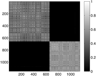
Figure 11. Probability of the event when two proteins are assigned to the same class when k = 5 classes are requested for the dimension 1 data. The probability is calculated for each pair of proteins by repeating the clustering multiple times and counting how many times the pairs were co-classified.

Last, Figure 12 illustrates the Wasserstein distances for the dimension two intervals. Similarly to the distances for the dimension one intervals, we can distinguish two blocks, the first four groups in the first block and the last group of configurations in a separate block. However, groups two and three (1CFD, 1FXD) seem to have relatively reduced distances to group five (1QB0) perturbing a bit the block-structure. If we look at the corresponding S(k) curve (Figure 13), we see that it indicates a single cluster as the best solution, probably because of the coupling of the groups two and three to the fifth group. Still, the jump of S(k) from k = 1 to k = 2 is less steep than the other increments, therefore we can consider a two-cluster structure. Performing the clusterings for k = 2 yields results presented in Figure 14. Indeed, we find the two clusters which correspond to the clusters found in Figure 10. However, if we try to find more clusters, as presented in Figure 15, we see that there is an underlying structure of the clusters, which contains three clusters, groups one and four (1A19, 1HOE) corresponding to one cluster, groups two and three (1CFD, 1FXD) to a second one while the fifth group (1QB0) is again separated from the rest forming its own cluster. This suggests a clustering which is influenced by the geometric size and other topological factors.

FIGURE 12

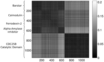
Figure 12. Wasserstein distances for the distributions representing the dimension 2 intervals. Each row and column corresponds to a protein-configuration, the ordering of the rows and the columns are the same. A darker shade means small distance while lighter shades implies larger distances. Not the dark blocks on the diagonal, they correspond to protein-groups which are close to each other.

FIGURE 13

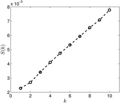
Figure 13. The S(k) curve for the clustering of the dimension 2 data, calculated based on equation (2).

FIGURE 14

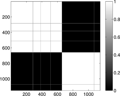
Figure 14. Probability of the event when two proteins are assigned to the same class when k = 2 classes are requested for the dimension 2 data. The probability is calculated for each pair of proteins by repeating the clustering multiple times and counting how many times the pairs were co-classified.

FIGURE 15

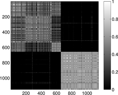
Figure 15. Probability of the event when two proteins are assigned to the same class when k = 5 classes are requested for the dimension 2 data. The probability is calculated for each pair of proteins by repeating the clustering multiple times and counting how many times the pairs were co-classified.

4. Discussion and Conclusions

We described a framework for analyzing and grouping molecules from a purely mathematical point of view. However, based on our arguments and the presented example, it is clear that this simple topological analysis has a much deeper meaning: it considers the topology and the geometry of the molecules within the same mathematical framework. Speaking about comparing proteins, in contrast to the currently available heuristic methods, our approach follows a nice and clear mathematical logic. It has a solid foundation, partially stemming from the field of computational topology and graph theory and partially based on methods of image processing, the Wasserstein distance being a standard tool in this field. It has been proven in the literature that the distance is a real metric, thus applying a k-means algorithm to find the different, topologically related groups in a given set of proteins is straightforward.

Using the framework for comparison, the method can be summarized in a few simple steps: First we analyze the structures and check for the presence of topological features like components, holes and voids, using a technique developed in computational topology for arbitrary point-clouds. Then we assess the similarity by statistically comparing the presence or absence of these features in the different molecules.

We presented a test-case, where these groupings are a priori known, being different foldings of some proteins. However, this knowledge did not constitute an input to our analysis and it was used only for validating the results. Our method was able to reveal the different ensembles with a high precision even though no chemical information was considered. The analysis was simply performed on the position of atoms. As it was demonstrated, a grouping which implies the geometry and size of the proteins is implicitly possible, without having to calculate best alignments.

We mention that the method can be tuned for different scopes by choosing the lower and the upper bounds of the l_c cutoff. For instance, we chose the largest edge in the triangulation as the biggest value for l_c. This leads to a coarse-graining procedure in which, when reaching larger scales, the geometry of the molecule is also encoded. If one uses the largest bond-length as the biggest cutoff, one, in fact, will compare molecular topologies and completely discard the information hidden in the folding of the molecule. Another possibility is to consider chemical information by applying the idea of fragment-based similarity [27] and represent a molecule in a high-dimensional space, where each axis corresponds to a pair of atom types, e.g., carbon–carbon, carbon–oxygen, carbon–hydrogen, oxygen–nitrogen, oxygen–oxygen, etc. Then, distances between any two atoms in a molecule along the backbone of the molecule can be represented as a point on the corresponding axis. Distances can be expressed in number of bonds, for instance. Selecting many different fragments of the molecule and representing the fragments in this space, we can build a point-set which is a chemical fingerprint of the molecule. Then we can calculate the barcodes of this point-set and apply our approach in a straightforward manner.

We believe that the presented framework can constitute the basis of a new approach or be a part of a methodology which is able to deal with flexibility of chemical structures in terms of similarity and dissimilarity. As there is no unique and well-defined way to classify proteins, we are convinced that such approaches are needed to open up different perspectives for researchers working in the field.

Conflict of Interest Statement

The authors declare that the research was conducted in the absence of any commercial or financial relationships that could be construed as a potential conflict of interest.

Acknowledgments

Gabriell Máté gratefully acknowledges support from the German Science Foundation (DFG) as a member of the Research Training Group “Spatio/Temporal Probabilistic Graphical Models and Applications in Image Analysis,” grant GRK 1653, the Heidelberg Graduate School of Mathematical and Computational Methods for the Sciences and the Institute for Theoretical Physics, all at the University of Heidelberg. Furthermore, the authors acknowledge the financial support of the Deutsche Forschungsgemeinschaft and Ruprecht-Karls-Universität Heidelberg within the funding programme Open Access Publishing.

References

1. van Westen GJP, Overington JP. A ligand's-eye view of protein similarity. Nat Methods. (2013) 10:116–7. doi: 10.1038/nmeth.2339

Pubmed Abstract | Pubmed Full Text | CrossRef Full Text

2. Nikolova N, Jaworska J. Approaches to measure chemical similarity – a review. QSAR Comb Sci. (2003) 22:1006–26. doi: 10.1002/qsar.200330831

CrossRef Full Text

3. Ballester PJ, Richards WG. Ultrafast shape recognition for similarity search in molecular databases. Proc R Soc A Math Phys Eng Sci. (2007) 463:1307–21. doi: 10.1098/rspa.2007.1823

CrossRef Full Text

4. Hasegawa H, Holm L. Advances and pitfalls of protein structural alignment. Curr Opin Struct Biol. (2009) 19:341–8. doi: 10.1016/j.sbi.2009.04.003

Pubmed Abstract | Pubmed Full Text | CrossRef Full Text

5. Liu YS, Fang Y, Ramani K. IDSS: deformation invariant signatures for molecular shape comparison. BMC Bioinform. (2009) 10:157. doi: 10.1186/1471-2105-10-157

Pubmed Abstract | Pubmed Full Text | CrossRef Full Text

6. Fober T, Mernberger M, Klebe G, Hüllermeier E. Graph-based methods for protein structure comparison. Wiley Interdiscip Rev Data Mining Knowl Discov. (2013) 3:307–20. doi: 10.1002/widm.1099

CrossRef Full Text

7. Teilum K, Olsen JG, Kragelund BB. Functional aspects of protein flexibility. Cell Mol Life Sci. (2009) 66:2231–47. doi: 10.1007/s00018-009-0014-6

Pubmed Abstract | Pubmed Full Text | CrossRef Full Text

8. Feinauer CJ, Hofmann A, Goldt S, Liu L, Máté G, Heermann DW. Chapter three - zinc finger proteins and the 3D organization of chromosomes. In: Donev R, editor. Organisation of Chromosomes. Advances in protein chemistry and structural biology, Vol. 90. Cambridge, MA: Academic Press (2013). p. 67–117. doi: 10.1016/B978-0-12-410523-2.00003-1

CrossRef Full Text

9. Wang Y, Fisher JC, Mathew R, Ou L, Otieno S, Sublet J, et al. Intrinsic disorder mediates the diverse regulatory functions of the Cdk inhibitor p21. Nat Chem Biol. (2011) 7:214–21. doi: 10.1038/nchembio.536

Pubmed Abstract | Pubmed Full Text | CrossRef Full Text

10. Gameiro M, Hiraoka Y, Izumi S, Kramar M, Mischaikow K, Nanda V. Topological Measurement of Protein Compressibility via Persistence Diagrams. MI preprint series. Global COE Program Math-for-Industry Education & Research Hub (2012).

11. Máté G, Hofmann A, Wenzel N, Heermann DW. A topological similarity measure for proteins. Biochim Biophys Acta. (2014) 1838:1180–90. doi: 10.1016/j.bbamem.2013.08.019

Pubmed Abstract | Pubmed Full Text | CrossRef Full Text

12. Carlsson G. Topology and data. Bull Amer Math Soc (NS). (2009) 46:255–308. doi: 10.1090/S0273-0979-09-01249-X

CrossRef Full Text

13. Edelsbrunner H, Harer J. Computational Topology – An Introduction. Providence, RI: American Mathematical Society (2010).

14. Delaunay B. Sur la sphère vide. Izvestia Akademii Nauk SSSR, Otdelenie Matematicheskikh i Estestvennykh Nauk. Bull Ac Sci USSR (1934) 6:793–800.

15. Hausmann JC. On the vietoris-rips complexes and a cohomology theory for metric spaces. In: Prospects in Topology Princeton, NJ: Princeton University Press (1994). Annals of mathematical studies, Vol. 138. Princeton, NJ: Princeton University Press (1995). p. 175–188.

16. Edelsbrunner H, Kirkpatrick D, Seidel R. On the shape of a set of points in the plane. IEEE Trans Inform Theor. (1983) 29:551–9. doi: 10.1109/tit.1983.1056714

CrossRef Full Text

17. Morozov D. Dionysus – A C++ Library for Computing Persistent Homology (2013). Available online at: http://www.mrzv.org/software/dionysus/. Accessed on 1 July 2013.

18. Nanda V. Perseus: The Persistent Homology Software (2012). Available online at: http://www.math.rutgers.edu/vidit/perseus.html. Accessed on 15 Oct 2012.

19. Tausz A, Vejdemo-Johansson M, Adams H. JavaPlex: A Research Software Package for Persistent (Co)homology (2011). Available online at: http://code.google.com/javaplex

20. Ghrist R. Barcodes: the persistent topology of data. Bull Am Math Soc. (2008) 45:61–75. doi: 10.1090/S0273-0979-07-01191-3

CrossRef Full Text

21. Csiszár I. Eine informationstheoretische Ungleichung und ihre Anwendung auf den Beweis der Ergodizitat von Markoffschen Ketten. Magyar Tud Akad Mat Kutató Int Közl. (1963) 8:85–108.

22. Kullback S, Leibler RA. On information and sufficiency. Ann Math Stat. (1951) 22:79–86. doi: 10.2307/2236703

CrossRef Full Text

23. Villani C. Topics in optimal transportation. In: Craig W, Ivanov N, Krantz SG, Saltman D, editors. Graduate Studies in Mathematics. Providence: American Mathematical Society (2003).

24. MacQueen JB. Some methods for classification and analysis of multiVariate observations. In: Cam LML, Neyman J, editors. Proceedings of the Fifth Berkeley Symposium on Mathematical Statistics and Probability, Vol. 1. Berkeley, CA: University of California Press (1967). p. 281–97.

25. Rubner Y, Tomasi C, Guibas LJ. A metric for distributions with applications to image databases. In Proceedings of the IEEE International Conference on Computer Vision; 1998 Jan 4–7; Bombay (1998). p. 59–66.

26. Zuckerman DM. The Ensemble Protein Database (2006). Available online at: http://www.epdb.pitt.edu/. Accessed on 1 July 2013.

27. Chen X, Reynolds CH. Performance of similarity measures in 2D fragment-based similarity searching: comparison of structural descriptors and similarity coefficients. J Chem Inform Comput Sci. (2002) 42:1407–14. doi: 10.1021/ci025531g

Pubmed Abstract | Pubmed Full Text | CrossRef Full Text