Lattice Boltzmann modeling of water-like fluids

1. Introduction

Water is a very special fluid, key to most human activities and life itself on our planet. As compared to standard fluids, water exhibits many anomalies, primarily the fact of being denser in the liquid than in the solid phase, exposing a density maximum above the freezing point, a large latent heat and heat capacity, high surface tension, and many others [1–3]. Although a fully comprehensive theory of water thermodynamics is still lacking, there is an increasing consensus that many of these anomalies can be traced back to the peculiar nature of the hydrogen bond (HB) [4, 5]. Indeed, the HB dynamics plays a vital role on structure formation within water. For instance, in water at low temperature, the HBs lead to the formation of an open, approximately four-coordinated (tetrahedral) structure, in which entropy, internal energy, and density decrease with decreasing temperature [1, 6, 7]. The equilibrium thermodynamics, i.e., phase diagram of water is exceedingly rich, and an Ab initio comprehensive analysis of its properties is still beyond computational reach. As a result, many models have been developed [8–11], including lattice ones displaying water-like behavior. Such lattice models are typically based on a many-body lattice-gas Hamiltonian mimicking the essential features of water interactions, with no claim (aim) of (at) atomistic fidelity [12]. To the best of our knowledge, these models have been employed mostly for the study of equilibrium properties, typically via Monte Carlo simulations. Yet, in most phenomena of practical interest, water flows and, most importantly, a variety of molecules, say colloids, ions, and biopolymers, flow along with it, typically in nano-confined geometries. In the biological context, it is well known that the competition between hydrophobic and hydrophilic interactions plays a crucial role in affecting the conformational dynamics of proteins [13–15]. On a larger scale, hydrodynamic interactions are known to exert a significant effect on the collective dynamics and aggregation phenomena within protein suspensions. More generally, hydrodynamic interactions are crucial in the presence of confining walls, due to their strong coupling with resulting inhomogeneities [16]. Based on the above, there is clearly wide scope for a minimal model of water behavior, capable of including hydrodynamic interactions and geometrical confinement.

A methodology to develop an appropriate multiscale approach to water modeling is offered by the Lattice Boltzmann method, a simulation technique based on a minimal form of Boltzmann kinetic equation living on a discrete space-time lattice [17–20]. Lattice Boltzmann equations have proven fairly successful in simulating a broad variety of complex flows across scales, from macroscopic fluid turbulence, all the way down to biopolymer translocation in nanopores [21, 22]. The lattice Boltzmann (LB) approach is mostly valued for its flexibility toward the treatment of complex geometries and seamless inclusion of complex physical interactions, e.g., flows with phase transitions, flows with suspended bodies, dynamics of droplets and many others [23–25]. The appeal of the method is due to its conceptual simplicity and computational efficiency, especially on parallel computers [26, 27]. Recently a LB model implementing the two-dimensional Ben-Naim model (BN2d) has been presented and applied to the simulation of simple confined water-like fluids [28]. In this paper, we present three-dimensional extensions dealing with both 3d Ben-Naim and TIP3P water potentials and explore the properties of such model in free space (bulk water). This serves as a preparatory step for future applications to complex situations involving nano-confinement and hydrodynamic interactions.

The paper is organized as follows. In section 2 we briefly mention the main classes of water models, from Ab initio molecular dynamics, to phenomenological lattice models. In section 3 we discuss the main ideas behind the LB for simple fluids, fluids with no internal structure. In section 4, we present the basic elements of our fluid model, while in section 5 we discuss the lattice implementation of the BN3d and TIP3P potentials. Section 6 then describes the dynamics of rotational degrees of freedom within a quaternion representation. Section 7 presents numerical results for various parametrization of the lattice BN3d potential, with special attention to the formation of hydrogen bonds in the course of the evolution, while section 8 describes dynamic energy minimization results. A summary and outlook are given in section 9.

2. Computational Modeling of Water

Like most complex dynamical systems, water can be modeled at different levels, seeking an optimal compromise between physical accuracy and computational efficiency.

At the most fundamental level, electronic and protonic degrees of freedom, essential to the hydrogen bond formation, are explicitly taken into account at quantum-mechanical level, along with the classical motion of oxygen ions. This Ab initio Molecular Dynamics (AiMD) approach is, however, very expensive, and currently limited to samples of about 100 molecules over trajectories spanning about 1 ns [29–33].

At the next level, the quantum-mechanical description is surrended in favor of empirical potentials, which release considerably the computational burden. Even so, world-record all-atom Molecular Dynamics (MD) simulations of protein folding in water, tracing the trajectory of roughly 10⁴ water molecules over 1 ms, takes several CPU months on the special-purpose supercomputer ANTON [34]. Substantial savings can be obtained by replacing all-atom solvent with implicit formulations, whereby the water solvent is treated like a dielectric continuum media, but at the expense of physical realism.

Finally, at a purely mesoscopic level, water is often represented as a collection of fields living on a discrete lattice and interacting according to stylized lattice Hamiltonians. Despite their minimality, such models have proved very valuable in exploring equilibrium properties of water via extensive Monte Carlo simulations [35–41]. The present paper falls within this latter class of lattice water models, with a few distinctive features, namely the possibility of including (1) full hydrodynamic interactions and (2) confined geometries.

The simulations discussed hereafter shall be restricted to periodic geometries with no net hydrodynamic motion. This responds to the need of calibrating the models against the existing literature, mostly Monte Carlo and Molecular Dynamics simulations. However, the mathematical formulation presented in the sequel is sufficiently general to encompass both items (1) and (2) above for future applications.

3. Lattice Boltzmann Representation of Fluid-Dynamics

The macroscopic dynamics of water is commonly described by the Navier–Stokes equations of continuum mechanics, whereas at a micro-nanoscopic scale the motion of water molecules is studied with the methods of Newtonian molecular dynamics. In this paper, we shall put forward a third avenue, based on a mesoscopic representation of water in terms of Boltzmann kinetic theory. In this representation, fluid dynamics is described by the probability distribution function (PDF) f(x, v; t) of finding a water molecule at given position in space x, at a given time t, with molecular velocity v. The Boltzmann PDF is a rather heavy-duty object, living as it does in seven dimensional phase-space, three for ordinary space, three for velocity space, plus time. Once the PDF is available, however, macroscopic fluid quantities are readily obtained by simple integrations in velocity space. For instance, by integrating upon all possible velocities, one obtains

$\begin{array}{cc}\rho \left(x;t\right)={\displaystyle \int f}\left(x,v;t\right)dv& (1)\end{array}$

which represents the fluid number density, i.e., the number of molecules per unit volume at time t. By the same token,

$\begin{array}{cc}u\left(x;t\right)=\frac{{\displaystyle \int f}\left(x,v;t\right)vdv}{\rho \left(x;t\right)}& (2)\end{array}$

represents the local fluid speed.

A practical question immediately arises: why should one solve a complicated equation in seven variables, given that macroscopic fluid dynamics lives in the much smaller three-dimensional space? In principle this looks like a truly self-inflicted pain.

The answer to this question is indeed far from obvious: in essence the point is that in the last decade highly stylized versions of the Boltzmann equation have been developed, in which velocity space is reduced to a handful of discrete velocities, usually denoted by c_i. As a result, instead of dealing with a six-dimensional PDF (leaving time aside), one generates dynamic equations for a relatively small set, typically of order 20, of three-dimensional discrete distributions

$f_i\left(x;t\right)\equiv f\left(x,v=c_i;t\right)$

Twenty is still larger than the number of hydrodynamic fields, typically five, for density, three fluid velocity components, and pressure. Hence, the bargain is still not obvious. The second and crucial point is the evolution of these discrete distributions can be formulated in terms of elementary hops from site to site in a regular lattice and subsequent site-by-site relaxation to a given local equilibrium. The resulting Lattice Boltzmann (LB) dynamics has been proven to offer major advantages as compared to the discretization of the Navier–Stokes equation. Among others, the main advantage is that information always travels along simple straight lines, defined by the so-called lightcones Δx_i = c_iΔt, where Δt is the discrete time-step of the lattice dynamics. This is much simpler than transport along the material fluid lines Δx_u = u(x; t) Δt, where the fluid velocity is often a very complex function of space and time. Because of this simplicity, the LB method has proved to be an outstanding performer for the simulation flows in complex geometries, especially on parallel computers. The reader interested in full details is kindly directed to the vast literature on the subject [17–20]. So much for the macroscopic side of LB.

Living at an intermediate level between continuum and atomistic descriptions, LB also has a second side, pointing toward the microscopic description. In this respect, the potential advantage of the LB formalism is its flexibility toward the inclusion of suitably coarse-grained features of the underlying microscopic physics, such as customized pseudo-potentials describing intermolecular interactions as a mesoscopic level, i.e., at space and time scale beyond reach for molecular dynamics.

In this paper, we shall make use of both faces of the LB method.

3.1. Coarse-Graining: From Lattice to Physical Space-Time Units

The LB method was born as a computational alternative to the numerical solution of the Navier–Stokes equations for macroscopic fluids. Later on, and not without some controversy, it has been extended to the realm of micro and nanofluidics. Such extensions command a careful analysis of the foundations of the method, since it is clear at the micro and nanoscale LB no longer enjoys the rigorous back-up of Chapman–Enskog asymptotic ensuring the correct hydrodynamic limit.

A description of the issues associated with these extensions goes beyond the scope of this paper. Here we shall only touch at the basic question of the conversion between LB and physical units, one which bears directly upon the degree of coarse-graining associated with the LB representation, which bears directly on its computational efficiency.

3.1.1. Space units

To fix the length units, a natural choice is to stipulate a coarse-graining ratio between the mesh-spacing and the range σ of the intermolecular potential:

$\begin{array}{cc}b=\frac{\Delta x}{\sigma },& (3)\end{array}$

where σ is typically of the order of 0.3 nm. As a result, each LB cell contains of the order of b³ molecules.

In macroscopic applications, with, say, Δx = 10⁻³ m, b³ ~ 10¹⁸, so that fluctuations are totally negligible. In microfluids, with, say, Δx = 10⁻⁶ m, each lattice cells still contains billions of water molecules. At the nanoscopic level, however, say Δx = 10⁻⁹ m, b³ ~ 30, and fluctuations play a relevant role.

The case b = 1, which we denote by molecular mesh-spacing (MMS) corresponds to one water molecule per water-like molecule, hence no spatial coarse-graining.

This is consequential to the idea of attaching a rigid-body structure (water-like molecule) to each LB cell, as it belongs to the sequel of the paper.

It is worth recalling that the idea of taking LB down to molecular length scales has been applied before, to perform head-on comparisons between LB and MD for the case of flows past nanosized obstacles [42]. Such studies highlighted that quantitative agreement between the two methods requires even sub-molecular mesh-spacing i.e., b < 1. This choice runs into an apparent paradox: each LB particle represents less than one water molecule!

The paradox is possibly lifted by recalling that LB also implies a form of time-average and the fact that f(x, v; t) represents a probability density, to be discussed in the following.

3.1.2. Time units

The conversion to time units proceeds as follows. The LB timestep is given by

$\begin{array}{cc}\Delta t=\frac{\Delta x^2}{\nu },& (4)\end{array}$

where ν is the physical kinematic viscosity. Taking ν = 10⁻⁶ m²/s in the MMS scenario, we obtain Δt ~ 0.1 ps, to be compared with the typical MD time-step, Δt_MD ~ 1 fs.

This is a gift of the LB time-marching scheme, which remains stable with discrete timesteps of the same order of the relaxation time.

This also informs us that each LB step collects an average over about 100 MD steps, thus implying the notion of time-average mentioned earlier on.

3.1.3. Mass, energy, and temperature units

The standard LB choice is to fix the mass units at the molecular mass of the species under consideration.

Since this paper is centered about the capability to form hydrogen bonds (HB), here we fix the energy units instead. In particular, the unit energy is set by the HB energy, about 10 kJ/mole, ϵ^HB = 1. This also fixes the mass and temperature units.

However, temperature calls for a few additional considerations. To this purpose, it is expedient to consider the so-called Boltzmann number [43], defined as:

$\begin{array}{cc}Bo=\frac{k_{B}T}{m{c}_s^2}{\left(\frac{d}{\Delta x}\right)}^3& (5)\end{array}$

where d is the mean intermolecular separation. This number can be taken as a dimensionless measure of the relative strength of energy fluctuations, ΔE/E, within a single LB cell. Hence, by definition, Bo → 0 denotes the macroscopic limit.

Assuming to a first approximation that the intermolecular separation in liquid water is basically the same as the interaction range, the Boltzmann number can also be rewritten as:

$\begin{array}{cc}Bo=\frac{k_{B}T}{m{c}_s^2}\frac{1}{b^3}& (6)\end{array}$

The first term at the rhs is dictated by the equation of state, and for a liquid under ordinary conditions it can be taken of the order of 1 (for an ideal gas, it is exactly 1). The second term is fixed by the spatial coarse-graining and, as previously discussed, for macroscopic or even microscopic flows, it takes pretty negligible values. For the present application, b = 1, and consequently, the condition Bo ≪ 1, which is necessary to either ignore fluctuations, or handle them as a weak perturbation, is naturally attained by the fact that in water at ambient temperature the thermal speed is about 1/3 of the sound speed, i.e., v²_T/c²_s ~ 0.1. However, for reasons of numerical stability, in the simulations this ratio is further lowered to about 10⁻³.

Since we take k_BT/mc²_s = 0.001, the Boltzmann number remains pretty small, Bo = 0.001, even though we do not perform any coarse-graining in space (b = 1). Given that in the absence of hydrodynamic motion, the rotational dynamics is arguably dominant over the translational one, we feel that the neglect of translational fluctuations (i.e., fluctuations in the stress tensor) is a pretty reasonable approximation. Although reasonable under the present circumstances, such an approximation should be lifted in view of future applications involving net hydrodynamic motion under confinement, where hydrodynamic stress cannot be neglected and might have an influence on the dynamics of HB formation. This is a challenging issues for future research, since, to the best of our knowledge, the condition b = 1 is not addressed by any of the existing formulations of fluctuating Lattice Boltzmann [43, 44].

3.1.4. Gain from coarse-grain

Having discussed the conversion from physical to LB units, it is apparent that the space-time coarse-graining factor, hence the potential computational gain, associated with LB as compared to MD, is approximately given by:

$\begin{array}{cc}G~100b^3=100& (7)\end{array}$

where 100 comes from the ratio of time-steps and b³ is the coarse-graining in space, b = 1 in our case.

The above equation is based on the assumption that the CPU cost of a LB and MD step be the same, which is probably short of a factor 10 against LB, since each LB cell interacts with 27 fixed neighbors instead of about twice as many time-changing neighbors of a typical MD simulation for the same potential.

The above relation shows that even taking no coarse-graining in space, LB can potentially offer at least two orders of magnitude savings vs. an atomistic simulation of water.

Realizing this potential in actual practice is, however, conditioned to the usual tradeoff: that the information projected away by the coarse-graining be inessential to the physics under inspection.

This can be only verified case-by-case by actual simulations.

4. The Lattice Boltzmann Model of Water-Like Fluids

We construct a mesoscopic model for water, geared to obey the incompressible Navier–Stokes equation in the macroscopic limit, namely:

$\begin{array}{cc}{\partial }_{t}u+u·\nabla u=\nu \Delta u-\nabla p& (8)\end{array}$

where u is the fluid velocity, p the fluid pressure and ν is the kinematic viscosity and density has been set to the conventional value ρ = 1, on account of the incompressibility condition [45]:

$\nabla ·u=0$

Instead of discretizing the NSE as a set of non-linear partial differential equations, it is expedient to solve a minimal lattice version of an underlying kinetic Boltzmann equation [17]. Our fluid model is based on an extension of the lattice Boltzmann method for ideal fluids. We use a three-dimensional lattice with 27 discrete velocities (including the cell-center), known as D3Q27 in the LB literature. The elementary cell of the D3Q27 lattice is reported in Figure 1 and the implications of the lattice connectivity on the tetrahedral structure of the water-like molecules shall be discussed later.

FIGURE 1

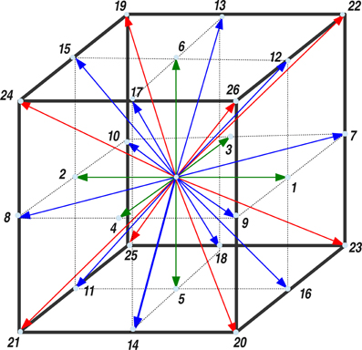
Figure 1. The unit cell of the D3Q27 lattice. The nearest neighbors, next-nearest neighbors and next-next nearest neighbors are shown in green, blue, and red, respectively. The weighting factors, w_i, for the D3Q27 are: w₀ = 8/27 (the cell-center), w_i = 2/27 (i = 1 − 6), w_i = 1/54 (i = 7 − 18), and w_i = 1/216 (i = 19 − 26).

At each grid node x, the velocity distribution function f_i(x; t), i.e., the probability to find a particle at location x, moving along the lattice direction defined by the discrete speed c_i, is evolved according to the lattice Bhatnagar-Gross-Krook model equation [46, 47]:

$\begin{array}{cc}{f}_i\left(x+c_i\Delta t,t+\Delta t\right)-f_i\left(x,t\right)=-\omega \left[f_i\left(x,t\right)-f_i^{eq}\left(x,t\right)\right]& (9)\end{array}$

where Δt is the time-step, ω = Δt/τ_LB and τ_LB is the relaxation time toward local equilibrium. The relaxation time fixes the fluid kinematic viscosity as follows:

$\begin{array}{cc}\nu =c_s^2\left({\tau }_{LB}-\Delta t/2\right)& (10)\end{array}$

where c_s is the sound speed of the lattice fluid. By taking Δx = Δt = 1, as it is customary in the LB literature, for the D3Q27 one has c_s = 1/$\sqrt{3}$. The local equilibrium distribution function is a Maxwellian, expanded to the second order in the fluid velocity:

$\begin{array}{cc}{f}_i^{eq}=\rho w_i\left(1+\frac{c_i·u}{c_s^2}+\frac{\left(c_i{c}_i-c_s^{2}I\right):\mathrm{uu}}{2c_s^4}\right)& (11)\end{array}$

where w_i is a lattice-dependent set of weighting factors, normalized to unit value and such that c²_s = ∑_iw_ic²_ia, a = x, y, z. The macroscopic observables, i.e., the fluid density and velocity are defined as follows:

$\begin{array}{cc}\rho \left(x,t\right)={\displaystyle \sum _i{f}_i}\left(x,t\right)& (12)\end{array}$

$\begin{array}{cc}\rho \left(x,t\right)u\left(x,t\right)={\displaystyle \sum _i{c}_i}{f}_i\left(x,t\right)& (13)\end{array}$

where mass has been set to unit value for convenience.

It is worth noting that the kinetic evolution of Equation (9) reproduces the macroscopic Navier–Stokes equation for small departures from local equilibrium, that is, when the Knudsen number Kn ~ (|f^eq − f|)/f ≪ 1. However, the small Kn condition is not strictly valid at mesoscopic level, since the mean free path of molecules is comparable with the intermolecular spacing. It is thus implicit in our treatment that the mesoscopic model can give rise to a non-hydrodynamic response on the small space/time scale. At numerical level, such regime receives substantial contributions from high-order kinetic moments and can give rise to spurious anisotropic effects arising from the finite number of discrete speeds that represent the distribution function [48].

5. Model Potentials for Water

In this section, we introduce two well-known potentials which are used for simulations of liquid water, and present the associated results from our LB simulations.

5.1. Lattice Three-Dimensional Ben-Naim (LBN3d) model

We model the interaction of water molecules on a lattice along the specifications given in Refs. [28, 49–51], i.e., the hydrogen bond interaction potential for two neighbor water molecules located at x_j and its neighbor along lattice direction i, x_i, as shown in Figure 2, based on three-dimensional Ben-Naim (BN3d) potential.

FIGURE 2

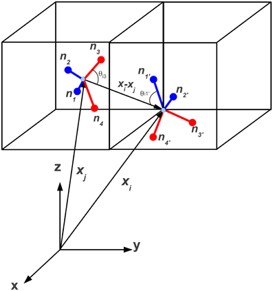
Figure 2. Tetrahedral representation of water-like molecules sitting at lattice site x_j and its neighbor x_i. The four arms are denoted by the corresponding normals n_k, k = 1, 4 (unprimed) and n_l, l = 1, 4 (primed), respectively. Blue and red code for donor and acceptor arms, respectively. Here the index i corresponds to i = 23 in Figure 1.

Although conceptually patterned after its two-dimensional predecessor [28], the three-dimensional extension requires significant technical upgrades [52], which we now proceed to illustrate. The BN3d potential, as presented in Hynninen [53], is given by:

$\begin{array}{cc}\begin{array}{l}V\left(x_j,x_i\right)={\displaystyle \sum _{k=1}^4{\displaystyle \sum _{l=1}^4{V}_{kl}}}\left(x_j,x_i\right)\\ =-G\left(r_i,\rho \right){\displaystyle \sum _{k=1}^4{\displaystyle \sum _{l=1}^4{ϵ}_{kl}^{HB}}}{e}^{-\frac{\left(W_{ik}+W_{il}\right)}{2{\sigma }_{\theta }^2}}.\end{array}& (14)\end{array}$

Note the minus sign in front of the potential, which connotates the global minimum as the most negative value. In the above, r_i = x_i − x_j is the distance between the centers of two neighbor tetrahedra, while ϵ^HB_kl is a selective matrix accounting for the fact that donor (acceptors) arms, corresponding to hydrogens (oxygens) may or may not be allowed to interact with each other. In the present study, all interactions have been enabled, including the repulsive ones, donor–donor and acceptor–acceptor. As a result, we set:

$\begin{array}{cc}{ϵ}_{kl}^{HB}=\mp 1& (15)\end{array}$

for repulsive (attractive) interactions, respectively. With this convention, repulsive(attractive) interactions contribute positive (negative) energy, respectively.

The radial interaction is chosen in the form [28]

$\begin{array}{cc}G\left(r_i;\rho \right)=W\left(\rho \right)e^{-\frac{1}{2}{\left(\frac{r_i-R_{HB}}{{\sigma }_R}\right)}^2}& (16)\end{array}$

where R_HB is the selected length of the hydrogen bond and σ_R controls the sharpness of the radial interaction. Each of the three choices, R_HB = 1, $\sqrt{2}$, $\sqrt{3}$, places a preferential bias on the formation of hydrogen bonds between face-centers (N2 = nearest-neighbors), edge-centers (N3 = next–nearest neighbors) or corners (N4 = next–next nearest neighbors) of the D3Q27 lattice, respectively. Note that each set of neighbors counts more than four sites, hence it can, in principle, saturate the four hydrogen bonds per molecule, with no extra contribution from other neighbors. The radial part of Equation (16) has been shown in Figure 3.

FIGURE 3

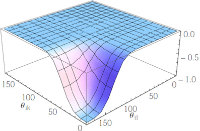
Figure 3. The angular potential V_ikl for σ_θ = 0.28. θ_ik and θ_il are shown in degrees.

In Equation (14), the density ρ(x_j) (at lattice site x_j) enters the weighting function through the empirical factor:

$\begin{array}{cc}W\left(\rho \right)\propto {\left(1+e^{-\alpha \left(\frac{{\rho }_{max}-\rho }{{\rho }_{max}-{\rho }_{min}}\right)}\right)}^{-1}& (17)\end{array}$

which takes into account the density-dependent propensity of water to form ordered states [28] at a lower density ρ_min, while the disordered states have a higher density ρ_max.

The parameter α > 0 controls the range of this density variation near solid walls, or due to salvation forces in the presence of any solute, Since in this paper we shall deal with bulk fluid only, without any solute, here and throughout we set α = 0, i.e., W(ρ) = 1.

The terms governing the directional interactions read as follows:

$\begin{array}{cc}{V}_{ikl}=e^{-\frac{W_{ik}+W_{il}}{2{\sigma }_{\theta }^2}}& (18)\end{array}$

where we have defined

$\begin{array}{cc}{W}_{ik}={\left({\widehat{n}}_k·{\widehat{r}}_i-1\right)}^2& (19)\end{array}$

and

$\begin{array}{cc}{W}_{il}={\left({\widehat{n}}_l·{\widehat{r}}_i+1\right)}^2.& (20)\end{array}$

These are the central objects governing directional interactions. The unit vector for the direction of the tetrahedral arm k, is denoted by ${\widehat{n}}_k=r_k/r_k$, while we have defined ${\widehat{r}}_i=r_i/r_i$ as the unit vector along the i-th link of the lattice. In the above, σ_θ is a parameter controlling the stiffness of directional interactions (small sigmas code for “stiff clicks”). It can be seen from Figure 2 that $n_k·{\widehat{r}}_i=\cos \left({\theta }_{ik}\right)$, where θ_ik is the angle between the k-th arm and the direction of the neighboring tetrahedron. The extremal values of V_ikl for σ_θ = 1 are reported in Table 1.

TABLE 1

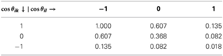
Table 1. Extremal values of the angular potential V_ikl ≡ e^{−(W_ik + W_il)/2σ2_θ}, corresponding to cos(θ_ik) = 1, 0, 1 and cos(θ_il) = 1, 0, 1 for the case σ_θ = 1.

Since W_ik + W_il takes values in the range [0, 8], the corresponding range of variation of V_ikl is [e^−4/σ2_θ, 1] for attractive interactions and [−1, −e^−4/σ2_θ] for repulsive ones (please note that the overall contribution is negative for attractive and positive for repulsive, on account of the minus sign upfronting the overall energy). This range exhibits a non-analytic dependence on the value of σ_θ. The angular potential V_ikl is reported in Figure 4 for the case σ_θ = 0.28. It can be noted that such case corresponds to a sharp (selective) landscape, taking the system toward the local minimum at cos θ_ik = 1 and cos θ_il = −1, respectively. Thus, to enforce sharp HB formation, σ_θ is selected to be sufficiently smaller than 1.

FIGURE 4

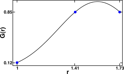
Figure 4. Radial shape functions for the case σ_R = 0.28 and R_HB = ($\sqrt{2}$ + $\sqrt{3}$)/2. Note that nearest-neighbor interactions are roughly an order of magnitude weaker than next and next–next nearest neighbor ones. The blue points show the value of radial shape function for r_i = 1, $\sqrt{2}$ and $\sqrt{3}$ corresponding to the nearest, the next–nearest and the next–next nearest neighbors, respectively.

5.2. Lattice TIP3P (LTIP3P) model

In the LTIP3P¹ model the potential of two neighboring molecules located at lattice nodes j and i, as shown in Figure 5, is given by

$\begin{array}{cc}V\left(x_j,x_i\right)=k_e{\displaystyle \sum _{k=1}^3{\displaystyle \sum _{l=1}^3\frac{Q_k{Q}_l}{\left|x_l-x_k\right|}}}& (21)\end{array}$

FIGURE 5

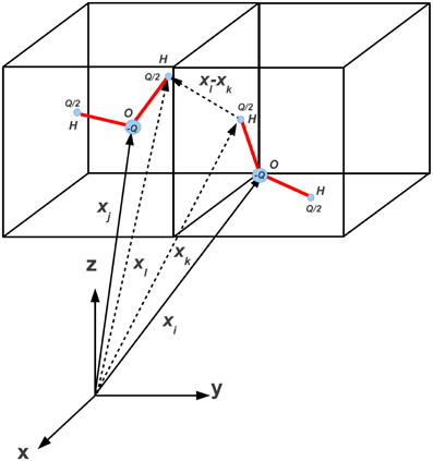
Figure 5. Illustration of two water molecules sitting at lattice site x_j and its neighbor x_i on the D3Q27 lattice in the LTIP3P model. The center of mass of the molecules is fixed at the lattice nodes.

in which k_e is the Coulomb's constant. The indices k and l refer to the charges of the water molecules associated with two hydrogens and one oxygen atoms for each molecule. Both hydrogens carry the same positive charge (+Q/2), while the oxygen carries a negative charge (−Q).

Since the center of mass of water-like molecules is fixed on lattice nodes at a distance of 2.77 Å, the Lennard–Jones potential is relatively weak as compared to the Coulomb potential and can therefore be neglected. We use the standard parameters for TIP3P water model given in the paper by Jorgensen and his coauthors [54]. Besides, the distance between the COM of a molecule with its nearest neighbor is fixed to 2.77 Å, as observed from molecular dynamics simulation of the bulk liquid [55]. In order to determine the full potential of a single molecule, we sum over the first shell of neighboring molecules only (26 molecules).

6. Equation of Motion of the Rotational Degrees of Freedom

At each lattice site, the water-like molecules perform rigid-body rotations under the drive of the torque associated with directional interactions with neighboring sites.

To compute such an effect, let us recall that the total potential energy of the water-like molecule sitting at lattice site x_j, is given by the sum of the pair potentials over the set of lattice neighbors, Equation (14), namely:

$\begin{array}{cc}V\left(x_j\right)={\displaystyle \sum _{i}V}\left(x_j,x_i\right)& (22)\end{array}$

The torque τ acting on the angular momentum ℓ of the water-like molecule placed at x_j, is given by:

$\begin{array}{cc}\tau ={\displaystyle \sum _{i=1}^{26}{\tau }_i}={\displaystyle \sum _{i=1}^{26}{\displaystyle \sum _{k=1}^{\chi }r}}\left(n_k\right)\times F_{ik}& (23)\end{array}$

where r(n_k) represents the position of the donor (or the acceptor) sitting at the tip of arm k and the force F_ik is given by the negative gradient of the potential energy of the arm k, due to the interaction with its ith neighbor, $-\nabla {\displaystyle \sum _{l=1}^{\chi }{V}_{ikl}}$ (see Equation 14). It should be noted that in LBN3d model χ = 4 and in LTIP3P model χ = 3. Since there is no radial dependence, it is convenient to calculate the force and the torque in spherical coordinates and then map the components back to the corresponding Cartesian coordinates (see Figure 6).

FIGURE 6

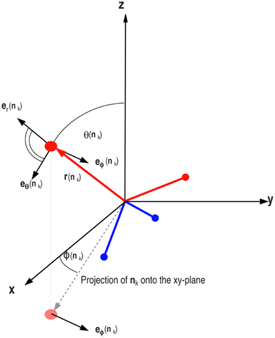
Figure 6. The torque acting on the arm n_k has two components in the direction of e_ϕ(n_k) and e_θ(n_k). The total torque acting on the tetrahedron is then the vector sum of the torques acting on all four arms in the LBN3d model.

We consider a driven-damped motion of the tetrahedron, according to the following Langevin equation:

$\begin{array}{cc}\stackrel{.}{\ell }=-\gamma \ell +\tau +{\tau }_r& (24)\end{array}$

where τ_r is a random component, encoding rotational diffusion effects. By construction, it obeys the fluctuation-dissipation relation:

$\begin{array}{cc}\langle {\tau }_r(t){\tau }_r(t^{\prime })\rangle =3\gamma {\beta }^{-1}I\delta (t-t^{\prime })& (25)\end{array}$

β being the effective temperature of the fluid (β⁻¹ ≡ k_BT), I the moment of inertia, a unit matrix of magnitude I, and δ is the delta function.

Next, we make the usual overdamping assumption, $|\stackrel{.}{\ell }|\ll \gamma |\ell |$, so that we may neglect the time rate of change of the angular momentum, to obtain:

$\begin{array}{cc}\omega =\frac{1}{\gamma I}\left(\tau +{\tau }_r\right)& (26)\end{array}$

where we have used the convention ℓ = Iω, so that $\ell =I\stackrel{.}{\varphi }$ Thus, by discretizing Equation (26), we have

$\begin{array}{cc}\Delta \varphi =\frac{\tau +{\tau }_r}{\gamma I}\Delta t.& (27)\end{array}$

This provides a rotation axis and a magnitude for the rotation around it, modulo 2π. The orientation of the tetrahedron is described by a quaternion with components q_μ [56], μ = 0, 1, 2, 3.

6.1. The Kinetic Equation for the Quaternion Moments

The quaternion macrofields q_μ(x, t) introduced in the previous section are assumed to obey the following transport equations:

$\begin{array}{cc}{\partial }_t{q}_{\mu }\left(x,t\right)+u·\nabla q_{\mu }\left(x,t\right)=D\Delta q_{\mu }+{\dot{q}}_{\mu }\left(x,t\right)& (28)\end{array}$

where u is the fluid velocity and D is the kinematic translational diffusivity of the quaternion components. The last term at the right hand side is the rate of change of the quaternion fields, due to the rigid-body rotation driven by the torque [56].

The idea behind the above equation is that the six translational and angular degrees of freedom are largely independent of each other, so the mean values of the angular degrees of freedom are simply advected by the mean flow and diffuse across it due to molecular collisions. This plausible approximation is necessary to turn around an otherwise intractable probability distribution of 12 independent variables, three position and three velocity coordinates, three angles and the corresponding three angular velocities.

The above equation is also solved by a Lattice Boltzmann technique, leading to the following set of kinetic equations:

$\begin{array}{cc}\begin{array}{l}{q}_{i\mu }\left(x+c_i\Delta t,t+\Delta t\right)=q_{i\mu }\left(x,t\right)\left(1-\frac{\Delta t}{\tau }\right)+q_{i\mu }^{eq}\left(x,t\right)\frac{\Delta t}{\tau }\\ +w_i{\dot{q}}_{\mu }\left(x,t\right)\Delta t\end{array}& (29)\end{array}$

where w_i are the lattice weights and c_i the lattice velocities introduced in section 3. In the above, τ is the quaternion relaxation time, controlling the kinematic diffusivity of quaternion according to

$\begin{array}{cc}D=c_s^2\left(\tau -1/2\right)& (30)\end{array}$

in lattice units Δt = Δx = 1.

Each component of the quaternion field, q_μ(x, t), is treated as the scalar density of a corresponding set of discrete distribution functions, according to:

$\begin{array}{cc}{q}_{\mu }\left(x,t\right)={\displaystyle \sum _i{q}_{i\mu }}\left(x,t\right)& (31)\end{array}$

In other words, each single component is treated as a fictitious density (note that this fictitious densities do not need to be positive definite). The local quaternion equilibrium in Equation 29 is given by

$\begin{array}{cc}{q}_{i\mu }^{eq}=w_i{q}_{\mu }\left(1+\frac{u·c_i}{c_s^2}\right)& (32)\end{array}$

in which the local velocity u is again provided by the coupled LB dynamics of the fluid. The quaternion components are updated concurrently with the LB fluid solver, and once this step is completed, the arms of the tetrahedron are updated accordingly. This way, the quaternion dynamics is coupled self-consistently to the hydrodynamic motion of the water-like fluid. We should mention that an imposed flow u, supplied by a standard LB scheme for fluid flow separately (introduced in section 3), does affect the quaternion dynamics (rotation of water molecules) via Equation 32 but the fluid flow itself is independent of the quaternion dynamics. In the current work we focus on the bulk water (no hydrodynamics) and set u = 0.

We wish to emphasize that even though the quaternion populations q_iμ live on lattice sites, their average (the actual physical observable), q_μ does not, as it is designed to obey the advection-diffusion-reaction equation (Equation 28). Thus, the observable rotational degrees of freedom are not bound to lattice sites. In particular, the relaxation time τ controls the translational diffusion of angular degrees of freedom, through Equation 30, while rotational diffusion is controlled by the strength of the noise in the Langevin equation for the angular momentum, Equations 26, 27.

7. Numerical Results

Any water-like model must necessarily pass a series of validation tests, depending on the application it is intended to. As a calibration of the present three-dimensional models, here we focus on their propensity to form hydrogen bonds under an optimal choice of simulation parameters.

7.1. Simulation Set-Up in the LBN3d Model

All simulations are performed on a D3Q27 lattice, with periodic boundary conditions. Initial conditions shall be discussed shortly. As noted earlier on, the D3Q27 lattice consists of three classes (“shells”) of sites: six face-centers at distance r = 1, 12 edge-centers at a distance r = $\sqrt{2}$, and eight corners at a distance r = $\sqrt{3}$. Unless stated otherwise, the simulations are performed with the following set of input parameters: σ_R = 0.28, σ_θ = 0.28, τ = 10³, γ = 10⁵ Δt⁻¹, τ_LB = 1, and R_HB = ($\sqrt{2}$ + $\sqrt{3}$)/2. The lattice consists of N_x = N_y = N_z = 10 grid points, for a total of 10³ lattice sites, each hosting a tetrahedral water-like molecule. Different values of the effective temperature are explored, approximately in the range between 10⁻⁴ ≤ β⁻¹ ≤ 10⁻³. All values are given in dimensionless LB units (Δx = Δt = 1). More precisely, initial conditions are taken random in the angular momentum, and then evolved at a low effective temperature (β⁻¹ = 10⁻⁴), until the system attains the condition HBs = 2. This transient thermalization helps minimizing trapping in local minima of the water potential associated with random initial conditions, which carry a low number HBs ≈ 0.2, very far from the global minimum at HBs = 4.

After such transient thermalization, the fluid configuration is further evolved at different values of the effective temperature, until a statistical steady-state is attained.

7.2. Dynamics of Hydrogen Bond Formation in LBN3d Model

In Figure 7, we show the time evolution of the water potential, Equation 17, with R_HB = ($\sqrt{3}$ + $\sqrt{2}$)/2, for the four effective temperatures: β⁻¹ = 10⁻⁴, β⁻¹ = 4 × 10⁻⁴, β⁻¹ = 5.5 × 10⁻⁴, and β⁻¹ = 7 × 10⁻⁴. The total energy of system is monitored, in order to appraise the tendency of the system toward minimum energy configurations. Technically, we stipulate that a hydrogen bond is formed whenever a donor and acceptor arms come head-on together, within a tolerance cone of aperture 20° [57].

FIGURE 7

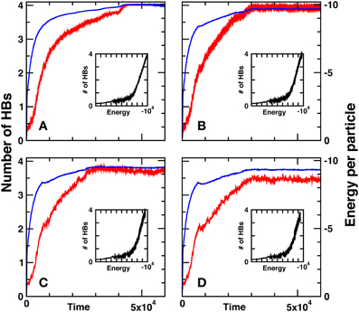
Figure 7. Time evolution of the total potential energy vs. the LB time steps together with the number of hydrogen bonds for four different effective temperatures, at (A) β⁻¹ = 10⁻⁴, (B) β⁻¹ = 4 × 10⁻⁴, (C) β⁻¹ = 5.5 × 10⁻⁴, and (D) β⁻¹ = 7 × 10⁻⁴. Main parameters are as follows N = 10³, σ_R = 0.28, σ_θ = 0.28, and R_HB = ($\sqrt{3}$ + $\sqrt{2}$)/2.

It should be noted that our results show sensitivity to the shape of radial interactions and sharing between competing shells of lattice molecules, so that a certain degree of fine-tuning is required. The choice R_HB = ($\sqrt{2}$ + $\sqrt{3}$)/2, is found to provide satisfactory results, with HBs pretty close to the top value, HBs = 4. Besides, the amplitude of thermal fluctuations depends on the choice of parameters in the BN3d potential particularly ϵ^HB_kl. High thermal fluctuations may corrupt the norm of quaternions, which must remain constant during the simulations, thus leading to numerical instabilities.

From Figure 7, it is apparent that a very substantial number of hydrogen bonds, nearing the top value HBs = 4, is formed at all effective temperatures, with a slight decrease at decreasing the effective temperature [5]. Also apparent is the strong correlation between the energy decrease (more negative) in time and the increasing number of hydrogen bonds, all along the simulation. This provides a neat indication that the number of hydrogen bonds serves indeed as a representative order parameter for the evolution of the system, from a high-energy disordered configuration to a quasi-ordered minimum-energy configuration.

7.3. Visual Information in LBN3d Model

To obtain a visual appreciation of the spatial ordering of the rotational degrees of freedom, the angular momenta, in Figure 8, we report the initial and the final configurations (steady state) of the water-like fluid at β⁻¹ = 10⁻⁴ and without thermal fluctuations. In case of no thermal fluctuations (Figure 8B), the final state is a highly ordered, ice-like crystal (HBs = 4). When thermal fluctuations are introduced (Figure 8C), the final configuration deviates from the crystal state (but still almost ordered) associated to a local minimum with a HBs <4, namely HBs ≃ 3.7. Clearly, the smaller β, the more pronounced is the deviation from an ordered crystal. Here, for the sake of a better visualization, the simulation has been performed for a small system of size N = 6³. The other LB parameters are the same as in the case of N = 10³.

FIGURE 8

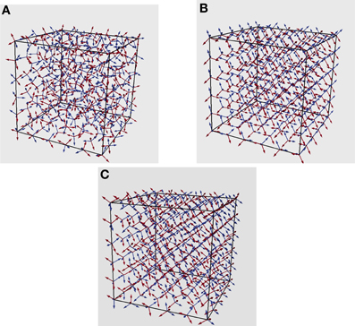
Figure 8. (A) Initial random distribution of tetrahedra and the corresponding final distribution at steady state with and without thermal fluctuations in (B,C), respectively.

7.4. Distribution of the HB Angle as a Function of the Temperature in LTIP3P Model

As we already mentioned, many water anomalies can be traced back to the nature and the particular geometry and structure of the hydrogen bonds (HB), which make and break within a very short lifetime. Considering the vital role of hydrogen bonding on the properties of water, here we focus on the angular distribution of hydrogen bonds in LTIP3P model. More results on the statistics of HB in LTIP3P model will be published elsewhere. A comparison with results of other studies can be regarded as a further validation of the current model. Here, we define the HB angle as the angle between the oxygen–oxygen connection line and the oxygen–hydrogen arm of two bonded (neighboring) water molecules. With this definition, a perfect HB angle corresponds to zero degrees. Our simulation results for the distribution of the HB angle at different temperatures is shown in Figure 9. It should be noted that our calculations were performed for the four best (smallest) HB angles for each molecule. For the sake of a better comparison we have renormalized our data in such a way that the highest distribution (which is known to occur at zero temperature) is taken to be 1.0.

FIGURE 9

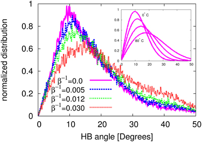
Figure 9. The normalized HB angle distribution at different temperatures in the LTIP3P model with β⁻¹ ≡ k_BT. In the inset the same distribution is presented using the data reported by Modig et al. [58].

As one can appreciate from the figure, the most probable angle goes from about 10^o at β⁻¹ = 0, to about 15° at β⁻¹ = 0.03. With the same HB definition and via an Ab initio density functional calculations, Modig and coauthors [58] have reported the HB angle in a temperature range between 0°C and 80°C. As a reference for the distribution of the HB angle as a function of temperature, we have reported the data from Modig's study in the inset of Figure 9. Comparing the present simulation results and the reference results by Modig et al. one can appreciate a qualitative agreement between the two studies. For example, in the case of no thermal fluctuations, 1/β = 0.0, our model and the results of Modig's study at zero degree both show a nearly zero value at HB angle = 0. Moreover, both results show a very similar increasing trend with the HB angle, reaching their maximum at an angle of about 10°. Finally they both decrease again to zero at an angle about 50°. A similar study has also been conducted (but with different HB angle definition) in Svishchev and Kusalik [59]. Our results are also qualitatively in line with the reported data in Svishchev and Kusalik [59].

We believe that such an agreement can be regarded as an additional validation of our water model and lends further credit to the current lattice approach for mesoscopic modeling of liquid water, at least for a certain class of applications.

8. Dynamic Minimization

We have run several simulations based on both LTIP3P and LBN3d, with different parameters. For the sake of validation, the same minimization problem has also been solved by an annealed Metropolis MC method.

8.1. LBN3d Simulations

In Figures 10A,B, we present the simulation results [energy in panel (A) and HBs in panel (B)] for a system size N = 6³, with γ = 10⁵ Δt⁻¹, at different τ and the same initial random distribution. For the case of LBN3d, we report the energy of the system in suitable dimensionless LB units, i.e., energy per pseudo-molecule divided by |ϵ^HB_kl|. We note that the optimum value of τ, meaning by this the value achieving the fastest energy minimization, depends on the potential, which explains why the optimum τ (τ/Δt = 1000) is different from the case of LTIP3P. As in the case of LTIP3P, in the early-time evolution only the over-relaxation regime (τ/Δt = 100 and τ/Δt = 1000) reaches the minimum, supporting faster minimization in the over-relaxation regime. Here, again the HBs increases with decreasing potential energy and reaches up to HBs = 4 [52]. Under all circumstances, it is seen that the optimum τ is always much larger than 1, indicating that LB operates best far from the hydrodynamic regime.

FIGURE 10

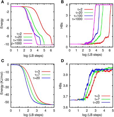
Figure 10. Energy and number of HB vs. LB steps at different τ: (A,B) for LBN3d and (C,D) for LTIP3P.

Here, we wish to observe that a nice property of LB is that beyond the hydrodynamic limit (τ ≫ 1), D is no longer proportional to τ, but actually becomes a non-local operator, leading to an effective diffusion which scales sub linearly with τ for τ ≫ 1 (see the reference by Blaak et al. 60). This is, we believe, the reason why LB delivers its best performance beyond the hydrodynamic limit. If D were too grow linearly with τ, for τ ≫ 1, it is unlikely that the scheme would still be able to capture the correct minimum.

8.2. LTIP3P Simulations

In Figures 10C,D, we have shown the total potential energy of the system in units of kJ/mol vs. the LB steps in panel (A) and their corresponding HBs in panel (B) at different τ but with the same initial random distribution. In the LTIP3P simulations, a hydrogen bond is considered to be formed when the distance between the donor H and the acceptor O is below 2.22 Å. This value represents the position of the first minimum of the OH radial distribution in our simulations, signaling a bonded state. Here, the system size is N = 10³ and the damping constant has been set to γ = 50 Δt⁻¹. From Figure 10, it is apparent that the simulation time to reach the global minimum for the largest τ is about a 100 times shorter than for the case of the lowest τ.

The long time behavior of the simulations shows that different τ finally lead to almost the same minimum, as well as the same HBs, confirming the consistency of the model. As it can clearly seen from the figure, our results indicate faster minimization in the over-relaxation regime. It can also be seen that the HBs increases with the decrease of the potential energy of the system, finally arriving at HBs ≈ 4, as expected [5].

We speculate that non-hydrodynamic operation is more efficient because “jumps” are long enough to avoid trapping in unfavorable minima, and at the same time, short enough to avoid overlooking the favorable ones. Here by “long enough,” we mean longer than those associated with standard local diffusion (τ ≫ 1), while “short enough” implies that beyond the hydrodynamic regime (τ ≫ 1), the effective non-local diffusivity associated with the LB dynamics scales sublinearly with the relaxation time τ (see comment in section 8.1).

This is the essence of kinetic over-relaxation: extreme but not too extreme. Simulations at high Knudsen numbers are not reproducing Equation 28, as they include higher order, isotropy-breaking, terms. However, since the goal is to attain the global minimum and not to reproduce the dynamics associated to a higher order versions of Equation 28, we are confident that our results are to a large extent insensitive to anisotropic effects. The above statement is indeed supported by quantitative comparison with Monte Carlo simulations as follows.

8.3. Comparison with Simulated Annealing Monte Carlo

In order to validate the model, we have compared our LB results with simulated annealing MC. In each MC sweep we randomly rotate the pseudo-molecules, and if the total potential energy of the system E is lower than the previous distribution, the move is accepted.

If not, the move is accepted with probability p ∝ e^−βE, where β is proportional to the inverse of temperature T⁻¹. In the annealed version, β is progressively increased during the MC simulation. In the present work, the MC scheme is characterized by three types of moves: (1) global rotations; (2) local rotation; (3) global refinement. In I each molecule rotates about a random axis by a random angle, chosen in the range [0°, 360°]. In (2), we randomly pick one water molecule and rotate it about a random axis by a random angle in the range [0°, 360°]. (3) is similar to (1), but the random angles are chosen in a narrower range [0°, 10°]. In Figure 11 we compare both cases, the LBN3d and the LTIP3P, with the simulated annealing MC discussed above. As it can be seen from the figure, in both cases LB attains the same minimum as in MC, which provides a validation of the LB model. Although our MC scheme can certainly be improved (no optimization has been carried out to ensure an optimal acceptance ratio between, say, 0.3 and 0.5), the computational performance of the LB minimizer remains remarkable.

FIGURE 11

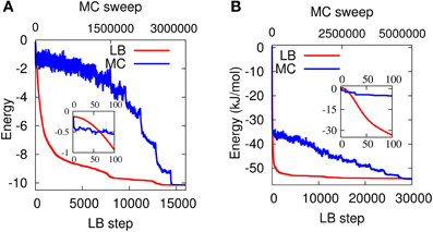
Figure 11. Energy vs. annealing MC sweeps (in blue) and LB steps (in red) for the LBN3d (A) and the LTIP3P (B). Both the MC and the LB methods reach the same minimum for the two potentials. In the case of LTIP3P, the main LB parameters are N = 10³, γ = 50 Δt⁻¹, and τ/Δt = 20 and in the case of LBN3d N = 6³, γ = 10⁵ Δt⁻¹, and τ/Δt = 1000. The insets show the very early LB steps/MC sweeps.

8.4. Time to Minimum vs. System Size

Two important quality factors of dynamic minimizers are their robustness toward changes in the initial conditions and the scaling of the time to solution with the size of the problem. The LB model is a deterministic minimizer, hence exposed to a sensitivity to the initial conditions for the minimization of highly corrugated potentials. However, this sensitivity can be strongly mitigated by a proper choice of LB parameters. On the other hand, owing to its strong locality, it features a remarkable linear scaling with the system size. As a result, the power of the LB minimizer is probably best displayed for large systems, a statement which is only accrued by the excellent amenability of LB scheme to parallel computing [61].

As it can be seen from Figure 12A, the LB model minimizes water energy based on the LTIP3P at different system sizes within nearly the same number of LB steps. Contrarily, as it can be seen from Figure 12B, the number of MC sweeps needed to reach the global minimum increases with the system size. Since the computational cost of the LB time-step scales linearly with the system size, we conclude that CPU time-to-minimum is also linear with the system size. This stands in notable contrast with annealed MC, where the number of sweeps to reach the global minimum grows rapidly with the system size [62]. Since each MC sweep takes about the same CPU time as a LB step, the end result is that LB becomes increasingly advantageous at larger system sizes. The simulations were performed on the same computer architectures and the comparison between MC and LB is based on pure observational evidence. Namely, we observed that the ratio of CPU time taken by a single LB step vs. a single MC sweep is about 1.5. This is plausible, because in both cases, most of the CPU time is taken by the calculation of the potential and torques, which is basically the same in the two cases. The next observation is that MC takes about 100 times more sweeps than LB steps to reach the global minimum. It should be further noted that even when LB does not reach the global minimum, due to a poor choice of the initial condition, it often attains a close-by local minimum.

FIGURE 12

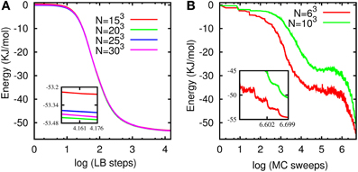
Figure 12. (A) Potential energy for the water model based on the LTIP3P vs. LB steps with τ/Δt = 20 (over-relaxation regime) and γ = 50 Δt⁻¹ for different system sizes. (B) Potential energy vs. (simulated annealing) MC sweeps for two different system sizes. The insets zoom into final energies.

As a result, one may envisage a synergistic coupling between LB as a fast quasi-global minimizer, to be combined with a subsequent MC minimization taking the system to its global minimum.

9. Conclusions and Future Prospects

Summarizing, we have presented a Lattice Boltzmann model of water-like fluids based on two well-known three-dimensional potentials for water simulations, BN3d and TIP3P.

The main results of the Lattice Boltzmann approach to water modeling presented here are as follows:

(1) The LBN3d model achieves a number of hydrogen bonds in the expected range, between 3 and 4. It also shows a sensitivity to the shape of radial interactions and sharing between competing shells of lattice molecules, so that a certain degree of parametric fine-tuning is required. The choice R_HB = ($\sqrt{2}$ + $\sqrt{3}$)/2 in LBN3d model, is found to provide satisfactory results, with HBs pretty close to the top value, HBs = 4 and a qualitatively correct dependence on the effective fluid temperature, if only in a limited range.

(2) Using TIP3P a qualitatively corrects statistics of the HB angle has been obtained as a function of the temperature.

(3) As an interesting bonus, the present LB scheme seems to act as a very effective a dynamic minimizer for the water-like lattice potential at hand. Under all conditions explored to date, many more than those reported in the present paper, it was able to find the near-global minimum starting from very far initial conditions, and typically significantly faster than annealed Monte Carlo. More importantly, perhaps, the time-to-minimum was found to scale linearly with the system size.

In the first place, a thorough series of validation test must be undertaken to identify which properties of real water can be reproduced to the desired level of accuracy: from water-like fluids to real water. In this paper we have discussed a key one, namely the capability to form hydrogen bonds, but many others need to be assessed, depending on the specific application at hand. Given the mesoscopic nature of the method, it is clear that each property may exhibit a different sensitivity to the degree of coarse-graining inherent to the LB representation (molecular individualism).

Once this validation/calibration campaign is completed, the model can be used to attack several prominent problems in computational chemistry and biology, for instance, a thorough investigation of the electrostatic properties, such as screening and dielectric behavior, are of utmost importance for a highly polar fluid such as water, or protein folding and aggregation at space and time scales beyond reach of atomistic simulations.

The present method, based on a minimally discretized version of the Boltzmann equation, leads to an efficient way of coarse-graining in time. This feature, together with the inherent efficiency of the lattice Boltzmann scheme, potentially allows to simulate water at larger length and time scales than molecular dynamics, without loosing (some of) the important microscopic features which control the main properties of water. Clearly, the latter statement must be constantly monitored against lattice discretization effects. Since the lattice Boltzmann discrete velocities have been designed to comply with the basic symmetries of continuum hydrodynamics, recovery of hydrodynamic behavior is automatically secured by the lattices used in this work, basically with second order accuracy in space and time. Should higher kinetic moments of the Boltzmann distribution play a major role on other properties of water, lattices with higher order symmetries will be required. Such lattices are available, as they have made the object of intense development in modern lattice Boltzmann theory. Given the broad use of lattice potentials in statistical mechanics, the approach described in this paper might open up an interesting direction for future research on multiscale simulations of micro and nano-biological phenomena.

The method also offers potential advantages vs. Monte Carlo, as it provides access to the non-equilibrium dynamics of the water-like fluid under heterogeneous hydrodynamic conditions. On the other hand, as compared with traditional models of lattice proteins, the present LB approach offers the advantage of coupling an explicit model of the solvent with hydrodynamic interactions, as combined with off-lattice representation of the protein. The present mesoscale approach may also open new perspectives for MM/QM multiscale simulations of complex chemical systems [63, 64].

Although extensive work is required to turn the above prospects into operational tools, the picture looks tantalizing.

Conflict of Interest Statement

The authors declare that the research was conducted in the absence of any commercial or financial relationships that could be construed as a potential conflict of interest.

Acknowledgments

Nasrollah Moradi acknowledges the funding from FRIAS. Andreas Greiner gratefully acknowledges funding from the University of Freiburg through an operating grant. Sauro Succi acknowledges financial support via the External Senior Fellow program at FRIAS.

Footnotes

1. ^The LTIP3P model has been discussed in details in a paper currently under review, available at: arXiv:1403.2432 [physics.comp-ph].

References

1. Errington JR, Debenedetti PG. Relationship between structural order and the anomalies of liquid water. Nature. (2001) 409:318. doi: 10.1038/35053024

Pubmed Abstract | Pubmed Full Text | CrossRef Full Text

2. Speedy RJ, Angell CA. Isothermal compressibility of supercooled water and evidence for a thermodynamic singularity at −45 ° C. J Chem Phys. (1976) 65:851. doi: 10.1063/1.433153

CrossRef Full Text

3. Pi HL, Aragones JL, Vega C, Noya EG, Abascal JLF, Gonzalez MA, et al. Anomalies in water as obtained from computer simulations of the tip4p/2005 model: density maxima, and density, isothermal compressibility and heat capacity minima. Mol Phys. (2009) 107:365. doi: 10.1080/00268970902784926

CrossRef Full Text

4. Luzar A, Chandler D. Hydrogen-bond kinetics in liquid water. Nature. (1996) 379:55. doi: 10.1038/379055a0

CrossRef Full Text

5. Kumar R, Schmidt JR, Skinner JL. Hydrogen bonding definitions and dynamics in liquid water. J Chem Phys. (2007) 126:204107. doi: 10.1063/1.2742385

Pubmed Abstract | Pubmed Full Text | CrossRef Full Text

6. Paschek D, Rüppert A, Geiger A. Thermodynamic and structural characterization of the transformation from a metastable low-density to a very high-density form of supercooled tip4p-ew model water. ChemPhysChem. (2008) 9:2737. doi: 10.1002/cphc.200800539

Pubmed Abstract | Pubmed Full Text | CrossRef Full Text

7. Garrett-Roe S, Rao F, Hamm P. Structural inhomogeneity of water by complex network analysis. J Phys Chem B. (2010) 114:15598. doi: 10.1021/jp1060792

Pubmed Abstract | Pubmed Full Text | CrossRef Full Text

8. Hamm P, Prada-Gracia D, Shevchuk R, Rao F. Towards a microscopic description of the free-energy landscape of water. J Chem Phys. (2012) 137:144504. doi: 10.1063/1.4755746

Pubmed Abstract | Pubmed Full Text | CrossRef Full Text

9. Vega C, Abascal JLF. Simulating water with rigid non-polarizable models: a general perspective. Phys Chem Chem Phys. (2011) 13:19663. doi: 10.1039/c1cp22168j

Pubmed Abstract | Pubmed Full Text | CrossRef Full Text

10. Barker JA. Lattice Theories of the Liquid State. Oxford, NY: Pergamon Press (1963).

11. Franzese G, Stanley HE. Liquid–liquid critical point in a Hamiltonian model for water: analytic solution. J Phys Condens Matter. (2002) 14:2201. doi: 10.1088/0953-8984/14/9/309

CrossRef Full Text

12. Pelizzola A, Buzano C, De Stefanis E, Pretti M. Two-dimensional lattice-fluid model with waterlike anomalies. Phys Rev E. (2004) 69:061502. doi: 10.1103/PhysRevE.69.061502

Pubmed Abstract | Pubmed Full Text | CrossRef Full Text

13. Karplus M. The Levinthal paradox: yesterday and today. Folding Des. (1997) 2:S69. doi: 10.1016/S1359-0278(97)00067-9

Pubmed Abstract | Pubmed Full Text | CrossRef Full Text

14. Cieplak M, Niewieczerzal S. Hydrodynamic interactions in protein folding. J Chem Phys. (2004) 342:299. doi: 10.1063/1.3050103

CrossRef Full Text

15. Rao F, Caflisch A. The protein folding network. J Mol Biol. (2009) 130:124906. doi: 10.1016/j.jmb.2004.06.063

Pubmed Abstract | Pubmed Full Text | CrossRef Full Text

16. Feibelman PJ. The first wetting layer on a solid. Phys Today. (2010) 63:34. doi: 10.1063/1.3326987

CrossRef Full Text

17. Succi S. The Lattice Boltzmann Equation. Oxford, NY: Oxford University Press (2001).

18. Wolf-Gladrow D. Lattice-Gas Cellular Automata and Lattice Boltzmann Models. New York, NY: Springer (2000). doi: 10.1007/b72010

CrossRef Full Text

19. Succi S, Benzi R, Vergassola M. The lattice Boltzmann equation: theory and applications. Phys Rep. (1992) 222:145. doi: 10.1016/0370-1573(92)90090-M

CrossRef Full Text

20. Chen S, Doolen G. Lattice Boltzmann method flow for fluid flows. Ann Rev Fluid Mech. (1998) 30:329. doi: 10.1146/annurev.fluid.30.1.329

CrossRef Full Text

21. Succi S. Lattice Boltzmann across scales: from turbulence to DNA translocation. Eur Phys J B. (2008) 64:471. doi: 10.1140/epjb/e2008-00067-3

CrossRef Full Text

22. Farahpour F, Maleknejad A, Varnik F, Ejtehadi MR. Chain deformation in translocation phenomena. Soft Matter. (2013) 9:2750. doi: 10.1039/c2sm27416g

CrossRef Full Text

23. Aidun CK, Clausen, JR. Lattice-Boltzmann method for complex flows. Annu Rev Fluid Mech. (2010) 42:439. doi: 10.1146/annurev-fluid-121108-145519

CrossRef Full Text

24. Moradi N, Varnik F, Steinbach I. Roughness-gradient–induced spontaneous motion of droplets on hydrophobic surfaces: a lattice Boltzmann study. EPL. (2010) 89:26006. doi: 10.1209/0295-5075/89/26006

CrossRef Full Text

25. Moradi N, Varnik F, Steinbach I. Contact angle dependence of the velocity of sliding cylindrical drop on flat substrates. EPL. (2011) 95:44003. doi: 10.1209/0295-5075/95/44003

CrossRef Full Text

26. Succi S, Amati G, Piva R. Massively parallel lattice-Boltzmann simulation of turbulent channel flow. Int J Mod Phys C. (1997) 8:869. doi: 10.1142/S0129183197000746

CrossRef Full Text

27. Mazzeo M, Coveney PV. HemeLB: a high performance parallel lattice-Boltzmann code for large scale fluid flow in complex geometries. Comput Phys Commun. (2008) 178:894. doi: 10.1016/j.cpc.2008.02.013

CrossRef Full Text

28. Mazzitelli I, Venturoli M, Melchionna S, Succi S. Towards a mesoscopic model of water-like fluids with hydrodynamic interactions. J Chem Phys. (2011) 135:124902. doi: 10.1063/1.3643326

Pubmed Abstract | Pubmed Full Text | CrossRef Full Text

29. Allesch M, Schwegler E, Gygi F, Galli G. A first principles simulation of rigid water. J Chem Phys. (2004) 120:5192. doi: 10.1063/1.1647529

Pubmed Abstract | Pubmed Full Text | CrossRef Full Text

30. Prendergast D, Grossman JC, Galli G. The electronic structure of liquid water within density-functional theory. J Chem Phys. (2005) 123:014501. doi: 10.1063/1.1940612

Pubmed Abstract | Pubmed Full Text | CrossRef Full Text

31. Grossman JC, Schwegler E, Draeger EW, Gygi F, Galli G. Towards an assessment of the accuracy of density functional theory for first principles simulations of water. J Chem Phys. (2004) 120:300. doi: 10.1063/1.1630560

Pubmed Abstract | Pubmed Full Text | CrossRef Full Text

32. Marx D, Tuckerman ME, Hutter J, Parrinello M. The nature of the hydrated excess proton in water. Nature. (1999) 397:601. doi: 10.1038/17579

CrossRef Full Text

33. Tuckerman ME, Marx D, Parrinello M. The nature and transport mechanism of hydrated hydroxide ions in aqueous solution. Nature. (2002) 417:925. doi: 10.1038/nature00797

Pubmed Abstract | Pubmed Full Text | CrossRef Full Text

34. Shaw DE, Maragakis P, Lindorff-Larsen K, Piana S, Dror RO, Eastwood MP, et al. Atomic-level characterization of the structural dynamics of proteins. Science. (2010) 330:341. doi: 10.1126/science.1187409

Pubmed Abstract | Pubmed Full Text | CrossRef Full Text

35. Bell GM. Statistical mechanics of water: lattice model with directed bonding. J Phys C Solid State Phys. (1972) 5:889. doi: 10.1088/0022-3719/5/9/004

CrossRef Full Text

36. Austen Angell C. Two-state thermodynamics and transport properties for water from bond lattice model. J Phys Chem. (1971) 75:3698. doi: 10.1021/j100693a010

CrossRef Full Text

37. Borick SS, Debenedetti PG, Sastry S. A lattice model of network-forming fluids with orientation-dependent bonding: equilibrium, stability, and implications for the phase behavior of supercooled water. J Phys Chem. (1995) 99:3781. doi: 10.1021/j100011a054

CrossRef Full Text

38. Pretti M, Buzano C. Thermodynamic anomalies in a lattice model of water. J Chem Phys. (2004) 121:11856. doi: 10.1063/1.1817924

Pubmed Abstract | Pubmed Full Text | CrossRef Full Text

39. Dias CL, Ala-Nissila T, Grant M, Karttunen M. Three-dimensional “Mercedes-Benz” model for water. J Chem Phys. (2009) 131:054505. doi: 10.1063/1.3183935

Pubmed Abstract | Pubmed Full Text | CrossRef Full Text

40. Bizjak A, Urbic T, Vlachy V, Dill KA. Theory for the three-dimensional Mercedes-Benz model of water. J Chem Phys. (2009) 131:194504. doi: 10.1063/1.3259970

Pubmed Abstract | Pubmed Full Text | CrossRef Full Text

41. Urbic T. Analytical model for three-dimensional Mercedes-Benz water molecules. Phys Rev E. (2012) 85:061503. doi: 10.1103/PhysRevE.85.061503

Pubmed Abstract | Pubmed Full Text | CrossRef Full Text

42. Horbach J, Succi S. Lattice Boltzmann vs. molecular dynamics simulation of nano-hydrodynamic flows. PRL. (2006) 96:224503. doi: 10.1103/PhysRevLett.96.224503

Pubmed Abstract | Pubmed Full Text | CrossRef Full Text

43. Duenweg B, Schiller U, Ladd A. Progress in the understanding of the fluctuating lattice Boltzmann equation. Comp Phys Commun. (2009) 180:605. doi: 10.1016/j.cpc.2009.01.014

CrossRef Full Text

44. Başaǧaoǧlua H, Melchionna S, Succi S, Yakhot V. Density fluctuations in lattice-Boltzmann simulations of multiphase fluids in a closed system. Europhys Lett. (2012) 99:64001. doi: 10.1016/j.physa.2006.08.002

CrossRef Full Text

45. Lev Davidovich Landau. Fluid Mechanics. Course of theoretical physics. Vol 6. Oxford, England: Pergamon Press Ltd. (1987).

46. Gross EP, Bhatnagar PL, Krook M. A model for collision processes in gases. I. Small amplitude processes in charged and neutral one-component systems. Phys Rev. (1954) 94:511. doi: 10.1103/PhysRev.94.511

CrossRef Full Text

47. Qian YH, D'Humieres D, Lallemand P. Lattice BGK models for Navier-stokes equation. EPL. (1992) 17:479. doi: 10.1209/0295-5075/17/6/001

CrossRef Full Text

48. Dellar P. Nonhydrodynamic modes and a priori construction of shallow water lattice Boltzmann equations. Phys Rev E. (2002) 65:036309. doi: 10.1103/PhysRevE.65.036309

Pubmed Abstract | Pubmed Full Text | CrossRef Full Text

49. Ben-Naim A. Statistical mechanics of “Waterlike” particles in two dimensions. I. Physical model and application of the Percus-Y evick equation. J Chem Phys. (1971) 54:3682. doi: 10.1063/1.1675414

Pubmed Abstract | Pubmed Full Text | CrossRef Full Text

50. Haymet ADJ, Silverstein KAT, Dill KA. A simple model of water and the hydrophobic effect. J Am Chem Soc. (1998) 120:3166. doi: 10.1021/ja973029k

CrossRef Full Text

51. Dias CL, Ala-Nissila T, Karttunen M, Vattulainen I, Grant M. Microscopic mechanism for cold denaturation. Phys Rev Lett. (2008) 100:118101. doi: 10.1103/PhysRevLett.100.118101

Pubmed Abstract | Pubmed Full Text | CrossRef Full Text

52. Moradi N, Greiner A, Rao F, Succi S. Lattice Boltzmann implementation of the three-dimensional Ben-Naim potential for water-like fluids. J Chem Phys. (2013) 138:124105. doi: 10.1063/1.4795008

Pubmed Abstract | Pubmed Full Text | CrossRef Full Text

53. Hynninen T, Dias CL, Mkrtchyan A, Heinonen V, Karttunen M, Foster AS, et al. A molecular dynamics implementation of the 3D Mercedes-Benz water model. Comput Phys Commun. (2012) 183:363. doi: 10.1016/j.cpc.2011.09.008

CrossRef Full Text

54. Jorgensen WL, Chandrasekhar J, Madura JD, Impey RW, Klein ML. Comparison of simple potential functions for simulating liquid water. J. Chem. Phys 79, 926 (1983). doi: 10.1063/1.445869

CrossRef Full Text

55. Mark P, Nilsson L. Structure and dynamics of the TIP3P, SPC, and SPC/E water models at 298 K. J Phys Chem A. (2001) 105:9954. doi: 10.1021/jp003020w

CrossRef Full Text

56. Rapaport DC. Molecular dynamics simulation using quaternions. Biophys Chem. (1985) 60:306.

57. Chaplin M. Water's Hydrogen Bond Strength. arXiv:0706.1355 [cond-mat.soft] (2007).

58. Modig K, Pfrommer BG, Halle B. Temperature-dependent hydrogen-bond geometry in liquid water. PRL. (2003) 7:075502. doi: 10.1103/PhysRevLett.90.075502

Pubmed Abstract | Pubmed Full Text | CrossRef Full Text

59. Svishchev IM, Kusalik PG. Structure in liquid water: a study of spatial distribution functions. J Chem Phys. (1993) 99:3049. doi: 10.1063/1.465158

CrossRef Full Text

60. Blaak R, Sloot PMA. Lattice dependence of reaction-diffusion in lattice Boltzmann modeling. Comput Phys Commun. (2002) 129:256. doi: 10.1016/S0010-4655(00)00112-0

CrossRef Full Text

61. Bernaschi M, Melchionna S, Succi S, Fyta M, Kaxiras E, Sircar JK. A parallel MUlti PHYsics/scale code for high performance bio-fluidic simulations. Comput Phys Commun. (2009) 180:1495. doi: 10.1016/j.cpc.2009.04.001

CrossRef Full Text

62. Doucet A, de Freitas N, Gordon N. Sequential Monte Carlo Methods in Practice. New York, NY: Springer (2001). doi: 10.1007/978-1-4757-3437-9

CrossRef Full Text

63. Kaxiras E, Succi S. Multiscale simulations of complex systems: computation meets reality. Sci. Model. Simul. (2009). 15:59. doi: 10.1007/s10820-008-9096-y

CrossRef Full Text

64. Scientific background on the Nobel Prize in Chemistry 2013 Development of multiscale models for complex chemical systems. (2013). Available online at: http://www.nobelprize.org/nobel_prizes/chemistry/laureates/2013/advanced-chemistryprize2013.pdf.

Pubmed Abstract | Pubmed Full Text