Effective rheology of Bingham fluids in a rough channel

1. Introduction

Yield-stress fluids, viz. fluids that require that the applied stress is above a non-zero threshold—a yield stress—for flowing [1], are found in many practical applications, such as in oil industry. Indeed, emulsions [2], mud [3, 4], heavy oil [5], polymeric gels such as carbopol [2] and foams [6] generate non-zero yield stress for flowing. In an oil recovery context, such fluids are injected to control premature production of water or gas. They do this by reducing poor sweep efficiency due to reservoir heterogeneities [7, 8]. Hydraulic fracturing operations—now very much a timely topic because of the increasing importance of fracking—involve also the flow of cross-linked polymer gels that are characterized by a yield stress to help carry proppant particles through the fractures. Common for these examples is that they occur in complex geometries; in the first in porous media, whereas in the second, the flow occurs inside rough cracks.

There have been a number of experimental [2, 9], numerical [10–16] and theoretical [17, 18] studies of the flow of yield stress fluids in porous media. One of the main objective is to derive an generalized Darcy equation for yield stress fluids relating mean flow rate, the pressure gradient and a critical pressure gradient. Experimentally [2, 9, 19] they establish various laws which have quite essentially the same structure,

$\begin{array}{cc}\Delta P-\Delta P_c\propto \{\begin{array}{l}\begin{array}{l}0\text{ if }\Delta P\le \Delta P_c,\\ Q^n\text{ if }\Delta P>\Delta P_c,\end{array}\hfill \end{array}& (1)\end{array}$

where Q is the total flow rate and n is the rheological exponent of the Herschel-Bulkley model. In particular, n = 1 defines the Bingham fluid. However, numerical simulations and pore-network models [15, 17, 20] demonstrate the situation may be much more complex that Equation (1) may be expected when the flow occurs in non-trivial geometries. Three different flow regimes,

$\begin{array}{cc}Q\propto {(\Delta P-\Delta P_c)}^{\alpha },& (2)\end{array}$

with α successively equal to 1, 2, and 1 for Bingham fluids when ΔP is increased beyond ΔP_c, may be identified. These three regimes are a consequence of the presence of heterogeneities in the pore size distribution and network topology.

In the present paper, we will study the different flow regimes in a one-dimensional (1D) rough channel. Besides offering interesting insights into the complexitites of the flow of yield stress fluids even in this seemingly simple case, it is of direct relevance in connection with flow both in two and three-dimensional porous media flow. Close to the yield threshold, there will be only one single one-dimensional channel where there is flow irrespecive of the dimensionality of the porous medium (see e.g., [11, 15, 17, 21]).

The present work relates to earlier work considering channel flow with periodically varying aperture [22–24]. In those articles, the authors investigated the validity of the lubrication approximation [25] which can become inconsistent with the presence of a unyielded plug along the center of the channel.

The main purpose of this paper is to investigate how Bingham fluids behave in one-dimensional channels with self-affine aperture variations. From earlier studies of how the permeability is affected by self-affine correlations in the aperture field [26], non-trivial scaling is to be expected of the parameters that characterize the flow also in this case.

A channel with a self-affine aperture field h(x) has an average aperture

$\begin{array}{cc}\langle h(x)\rangle \propto L^H,& (3)\end{array}$

where L is the distance along the channel over which the average is taken and H is the Hurst exponent [26]. We will later on this this paper present a more precise definition. Fractures are typically self affine (see e.g., [27–30]).

In the case of Newtonian flow in a channel with self-affine aperture correlations, it was enough to analyze the scaling properties of the permeability to have a full overview of what effect such correlations have on the flow. In the present case, it is necessary to expand the analytical solutions in power series. Each term in this series shows different scaling behavior.

The outline of the paper is as follow. In section 2, we consider flow in a one-dimensional rough channel in the lubrication limit. We solve the flow equations analytically and find flow rate as function of pressure difference across the length of the channel. After identifying a length scale associated to the flow rate, we use this length to expand in power series for small and large values of it, our analytical solution. In section 3, we discuss briefly our solution for a channel aperture that follows a cosine variation. In section 4, which contains the main results of this paper, we consider the roughness to be self affine and derive scaling relations between aperture, length of the channel and the length scale associated with the flow rate. In comparison to the Newtonian case, the scaling properties are much more subtle in this case due to the presence of the length scale, a*, characterizing the flow. We use the series expansions of section 2 to determine how each term scales. Finally, we propose in section 5 a truncated version of the double series expansion which reproduces the analytical solution over the entire range of flow rates. This is very useful as it is necessary to use such series to characterize the scaling properties of the flow equations when the aperture field is self affine. Section 6 contains our conclusions.

2. Bingham Flow in a Rough Channel: General Results

The Bingham yield threshold fluid [1, 31] has as constitutive equation

$\begin{array}{cc}{\dot{\gamma }}_{xy}=\{\begin{array}{cc}\frac{1}{D}\left({\sigma }_{xy}-\text{sgn}({\sigma }_{xy}){\sigma }_c\right)& \text{if |}{\sigma }_{\text{xy}}\text{|}>{\sigma }_{\text{c}},\\ \text{0}& \text{if |}{\sigma }_{\text{xy}}\text{|}\le {\sigma }_{\text{c}},\end{array}& (4)\end{array}$

where $\dot{\gamma }$_xy is the shear rate, σ_xy is the shear stress, σ_c is the shear stress yield threshold, D is the viscosity and sgn is the sign function.

By integrating the flow equations across the channel with the constitutive law given in Equation (4), we find for for position x along the channel where the aperture is h = h(x) that the total flow rate Q per unit of width is given by

$\begin{array}{cc}Q=-\frac{h^3}{12D}{p}^{\prime }{\left(1-\left|\frac{{p^{\prime }}_c}{p^{\prime }}\right|\right)}^2\left(1+\frac{1}{2}\left|\frac{{p^{\prime }}_c}{p^{\prime }}\right|\right),& (5)\end{array}$

where p′ = p′(x) is the pressure gradient at x. We have also defined a local pressure gradient threshold p′_c = p′_c(x) given by

$\begin{array}{cc}{p^{\prime }}_c=\frac{2{\sigma }_c}{h}.& (6)\end{array}$

We have here implicitly made the assumption that h(x) varies slowly enough so that the lubrication limit is in effect [23].

We may non-dimensionalize the flow Equation (5) by introducing a dimensionless pressure

$\begin{array}{cc}\overline{p^{\prime }}=\frac{p^{\prime }}{{p^{\prime }}_c}& (7)\end{array}$

and the inverse of the local Bingham number:

$\begin{array}{cc}\overline{Q}=\frac{DQ}{2{\sigma }_c{h}^2}.& (8)\end{array}$

Which quantify the balance between the viscous and yield stresses contributions at the scale h. Equation (5) then reads

$\begin{array}{cc}\overline{Q}=-\frac{1}{12}\overline{p^{\prime }}{\left(1-\frac{1}{\left|\overline{p^{\prime }}\right|}\right)}^2\left(1+\frac{1}{2\left|\overline{p^{\prime }}\right|}\right).& (9)\end{array}$

We solve this equation with respect to p′ and find

$\begin{array}{cc}\overline{p^{\prime }}=-\frac{\text{sgn}(\overline{Q})}{2}\left(1+8\left|\overline{Q}\right|\right)\left(1+2\cos \left[\frac{2}{3}{\csc }^{-1}\left({\left(1+8\left|\overline{Q}\right|\right)}^{3/2}\right)\right]\right)\text{}.& (10)\end{array}$

By integrating this equation over the length of the channel, we express the total flow rate Q as a function of the pressure drop over the total channel length L,

$\begin{array}{cc}\Delta P={\displaystyle {\int }_0^L{p}^{\prime }}(x)dx.& (11)\end{array}$

Hence, using Equations (7), (8), and (10) we find

$\begin{array}{cc}\begin{array}{l}\Delta P=-{\displaystyle {\int }_0^L}dx\text{sgn}(\text{Q})\frac{{\sigma }_c}{h(x)}\left(1+\frac{4D\left|Q\right|}{{\sigma }_{c}h{(x)}^2}\right)\\ \left[1+2\cos \left(\frac{2}{3}{\csc }^{-1}\left[{\left(1+\frac{4D\left|Q\right|}{{\sigma }_{c}h{(x)}^2}\right)}^{3/2}\right]\right)\right].\end{array}& (12)\end{array}$

We note that |ΔP| → P_c as |Q| → 0 in this equation, where

$\begin{array}{cc}{P}_c={\displaystyle {\int }_0^{L}d}x{p^{\prime }}_c(x)=2{\sigma }_c{I}_1(L).& (13)\end{array}$

We have here used Equation (6) and defined

$\begin{array}{cc}{I}_1(L)={\displaystyle {\int }_0^L\frac{dx}{h(x)}}.& (14)\end{array}$

P_c is the minimum pressure drop needed so that |Q| > 0 when |ΔP| > P_c. It is worthwhile to derive this threshold pressure from direct physical arguments since the result is not obvious.

Let us pick two positions along the channel, one at x₁ and the other at x₂. Here the threshold pressures are respectively p′_c1 and p′_c2. Since this is a channel, the total flux Q is the same everywhere along it. With reference to Figure 1, we now assume that the total flux is Q_a. Correspondingly the pressure gradient at position x_a is p′_1a and at position x₂ it is p′_2a. If we lower the total flux to Q_b we respectively find corresponding lower pressure gradients p′_1b and p′_2b at x₁ and x₂ respectively. We see from the figure that as the total flux Q → 0, p′₁ reach the threshold value p′_c1Âăexactly as p′₂ reaches p′_c2. Hence, as the total flux reaches zero all along the channel, the local pressure gradients reach their threshold values simultaneously. Equation (13) then follows since the total pressure as Q → 0 then must be the integral over the local threshold pressure gradients.

FIGURE 1

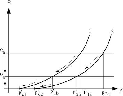
Figure 1. Labels “1” and “2” refer to two positions along a one-dimensional channel. The pressure gradient thresholds are p′_c1 and p′_c2 respectively. The total flow rate through the channel is the same at all positions. Hence, when the total flow rate is Q_a, there will be a corresponding pressure gradient p′_1a at position 1 and a pressure gradient p′_2b at position 2. When the total flow rate is lowered to Q_b, the pressure gradients become p′_1b and p′_2b at positions 1 and 2 respectively. From the figure, we see that as Q → 0, the pressure gradients p′₁ and p′₂ reach their respective thresholds, p′_c1 and p′_c2, simultaneously.

We now return to Equation (10). We may expand it for small |Q|. We find

$\begin{array}{cc}\overline{p^{\prime }}=-\text{sgn}(Q)\left[{\displaystyle \sum _{k=0}^{\infty }{a}_k}{\left(\sqrt{\left|\overline{Q}\right|}\right)}^k\right],& (15)\end{array}$

where a₀ = 1, a₁ = $\sqrt{8}$, a₂ = 16/3, and a₃ = 40$\sqrt{2}$/9.

If we keep only two terms in this series, reintroduce the original variables and integrate along the x axis, we find

$\begin{array}{cc}Q=-\frac{\text{sgn}(\Delta P)}{16{\sigma }_{c}D{I}_2{(L)}^2}\{\begin{array}{c}\begin{array}{l}\begin{array}{cc}0& \text{ if }|\Delta P|<P_{c,eff},\end{array}\\ \begin{array}{cc}{(|\Delta P|-P_{c,eff})}^2& \text{if }|\Delta P|\ge P_{c,eff},\end{array}\end{array}\end{array}& (16)\end{array}$

where

$\begin{array}{cc}{I}_2(L)={\displaystyle {\int }_0^L\frac{dx}{h{(x)}^2}},& (17)\end{array}$

and P_c is given by Equation (13). Hence, close to the threshold pressure, the flux is quadratic in the excess pressure.

Let us now introduce a length scale a* defined as

$\begin{array}{cc}{a}^{*}=\sqrt{\frac{D|Q|}{2{\sigma }_c}}=|\overline{Q}{|}^{1/2}h.& (18)\end{array}$

We have used here that Q is a constant along the length of the tube, and therefore Q varies with x. a* characterizes the flow everywhere along it and is independent of x. Hence, |Q| ≪ 1 is equivalent to a* ≪ h(x) and vice versa |Q| ≫ 1 is equivalent to a* ≫ h(x) for all x.

The series expansion (15) may then be transformed into the small-a* expansion

$\begin{array}{cc}\Delta P=-2{\sigma }_c\text{sgn}(Q){\displaystyle \sum _{k=0}^{\infty }{a}_k}{(a^{*})}^k{I}_{k+1}(L),& (19)\end{array}$

where we have defined

$\begin{array}{cc}{I}_k(a,L)={\displaystyle {\int }_0^L}\frac{dx}{h{(x)}^k}={\displaystyle {\int }_0^L\frac{dx}{{(a+\eta (x))}^k}},& (20)\end{array}$

where we have split the channel aperture into two components,

$\begin{array}{cc}h(x)=a+\eta (x),& (21)\end{array}$

where

$\begin{array}{cc}a=\underset{x}{\min }h(x),& (22)\end{array}$

and

$\begin{array}{cc}\eta (x)=h(x)-a.& (23)\end{array}$

All the geometrical information on the channel is now found in the integrals I_k(a, L). The information on the flow is encoded in the length scale a*.

In the other limit, Q ≫ 1, Equation (10) may be expanded as

$\begin{array}{cc}\overline{p^{\prime }}=-\text{sgn}(Q)\left[12|\overline{Q}|+\frac{3}{2}+{\displaystyle \sum _{k=2}^{\infty }{b}_k}{\left(\frac{1}{|\overline{Q}|}\right)}^k\right],& (24)\end{array}$

where b₂ = −1/288, b₃ = 1/1152 and so on. We introduce the length scale a* (18) in this expression and find

$\begin{array}{cc}\begin{array}{l}\Delta P=-2{\sigma }_c\text{sgn}(Q)[12{(a^{*})}^2{I}_3(a,L)+\frac{3}{2}{I}_1(a,L)\\ +{\displaystyle \sum _{k=2}^{\infty }\frac{b_k}{{(a^{*})}^{2k}}}{I}_{1-2k}(a,L)],\end{array}& (25)\end{array}$

which is then a large-a* expansion.

With only the dominating term, proportional to (a*)², included in this equation, we recover the Darcy equation with viscosity ν = D. Hence, the permeability is controlled by the integral I₃(L), as has already been discussed in Balhoff et al. [26].

It is interesting to note that the term corresponding to Darcy flow is present both in the large a* and the small a* expansions. It needs to be present in the large-a* expansion even though it is proportional to (a*)² since the Bingham fluid approaches the Newtonian limit with increasing flow rate.

Keeping the two leading terms and reverting to the original variables gives the equation

$\begin{array}{cc}Q=-\frac{\text{sgn}(\Delta P)}{12D{I}_3(a,L)}\{\begin{array}{c}\begin{array}{l}0\text{ if }|\Delta P|<P_{c,eff},\\ (|\Delta P|-P_{c,eff}),\text{ if }|\Delta P|\ge P_{c,eff},\end{array}\end{array}& (26)\end{array}$

where

$\begin{array}{cc}{P}_{c,eff}=\frac{3}{2}{P}_c,& (27)\end{array}$

where P_c is the threshold pressure. Hence, the fluid behaves as a linear fluid, but with an effective pressure threshold that must be overcome for flow to occur. The effective threshold is larger than the real flow threshold P_c as one would expect. Equation (26) is the approximation used e.g., by Roux and Herrmann [17] in their study of Bingham fluids in disordered networks. Since the effective pressure threshold, Equation (27) is proportional to the real threshold, it is still given by Equation (14). This justifies the approach of Roux and Herrmann [17].

3. Periodic Aperture Variations

Both expansion (19) and (25) are applicable for any aperture distribution, as long as the lubrication approximation remains valid. As example, following Frigaard et al. [23, 24] who considered an aperture varying according to a cosine function. We may then calculate I_k(a, L) analytically. We consider k = 1, 2, and 3.

Considering the aperture

$\begin{array}{cc}h(x)=a+\eta (x)=a+b+b\cos \left(\frac{2\pi Nx}{L}\right)\text{with}x\in [0,L],& (28)\end{array}$

where b is the amplitude of the aperture variation and N is the number of wavelengths in all. We then have

$\begin{array}{cc}\begin{array}{l}{I}_1=\frac{L}{\sqrt{a(a+2b)}},\\ I_2=\frac{L(a+b)}{{\left[a(a+2b)\right]}^{3/2}},\\ \text{and}{I}_3=\frac{L\left(2a^2+4ab+3b^2\right)}{2{\left[a(a+2b)\right]}^{5/2}}.\end{array}& (29)\end{array}$

Hence, the threshold pressure is then

$\begin{array}{cc}{P}_c=2{\sigma }_c\frac{L}{\sqrt{a(a+2b)}},& (30)\end{array}$

and the two limit expansions (19) and (25) to leading order are

$\begin{array}{cc}\Delta P\simeq -\text{sgn}(Q)(2{\sigma }_c{I}_1+4I_2\sqrt{{\sigma }_{c}D}\sqrt{|Q|})\text{for}Q\to 0& (31)\end{array}$

$\begin{array}{cc}\Delta P\simeq -\text{sgn}(Q)(12D{I}_3|Q|+3{\sigma }_c{I}_1)\text{for}Q\to \infty .& (32)\end{array}$

4. Self-Affine Apertures

A large number of studies report that the roughness of fracture surfaces show self-affine correlation [27–30]. We consider here the flow in a channel with aperture h(x) with a self-affine properties. This means that the aperture is characterized by a two point function p₂(h₂ − h₁, x₂ − x₁) giving the probability density that if h(x₁) = h₁ then h(x₂) = h₂. Self affinity is the scaling property

$\begin{array}{cc}{\lambda }^H{p}_2\left({\lambda }^H(h_2-h_1),\lambda (x_2-x_1)\right)=p_2\left(h_2-h_1,x_2-x_1\right)\text{}.& (33)\end{array}$

Normally, we have that 0 < H < 1.

In an earlier study [26], we considered the flow of a newtonian fluid in a channel where the aperture field obeyes the scaling relation (33). After identifying a length scale a characterizing the aperture opening (to be defined below), the permeability K relating flow rate Q to pressure difference along the channel, ΔP, scales as K ~ a^κ. For small a, κ = 3, for intermediate a, κ = 3 − 1/H and for large a, κ = 3. The question we pose here is: how does the the self affinity of the aperture field influence the equation relating Q and ΔP for a Bingham fluid.

The channel aperture is split into two components, h(x) = a + η(x), where the minimum aperture is a = min_x h(x) and η(x) is self affine characterized by a Hurst exponent H. Since we are in the lubrication limit, we may reshuffle the aperture field η(x) → η[ξ] = η(x(ξ)) where we have used an ordering transformation such that η(ξ₁) ≤ η(ξ₂) if ξ₁ < ξ₂. The averaged ordered sequence obeys the scaling law [26]

$\begin{array}{cc}\overline{\eta }[\xi ]={\xi }^H,& (34)\end{array}$

where we have set a prefactor equal to unity.

The fundamental integrals (20) that control the transport equations may then be written

$\begin{array}{cc}\begin{array}{l}{I}_k(a,L)={\displaystyle {\int }_0^L\frac{dx}{h{(x)}^k}}={\displaystyle {\int }_0^L\frac{d\xi }{{(a+{\xi }^H)}^k}}\\ =\frac{L}{a}{(a+L^H)}^{1-k}{}_2{F}_1\left(1,1+\frac{1}{H}-k;1+\frac{1}{H},-\frac{L^H}{a}\right),\end{array}& (35)\end{array}$

where ₂F₁ is the Gaussian hypergeometric function.

First we assume k > 0 in (35). For large a ≫ L^H, the integral is proportional to La^−k.

For intermediate to small values of a ≪ L^H, we may rewrite the integral

$\begin{array}{cc}{I}_k(a,L)=a^{1/H-k}{\displaystyle {\int }_0^{L/a^{1/H}}}\frac{d\xi }{{(1+{\xi }^H)}^k}.& (36)\end{array}$

Depending on whether kH is smaller than or larger than one, the integral will be dominated by the upper or lower integration limit. Hence, if kH < 1, the integral behaves as

$\begin{array}{cc}{\displaystyle {\int }_0^{L/a^{1/H}}\frac{d\xi }{{\xi }^{kH}}}\propto {\left(\frac{L}{a^{1/H}}\right)}^{1-kH}=L^{1-kH}{a}^{-1/H+k}.& (37)\end{array}$

This leads to

$\begin{array}{cc}{I}_k(a,L)=L^{1-kH}{a}^0.& (38)\end{array}$

On the other hand, if kH > 1, the integral will be dominated by the lower limit, and it does not depend on L nor a. We may summarize this,

$\begin{array}{cc}{I}_k(a,L)\propto \frac{L^{\max (1-kH,0)}}{a^{\max (kH-1,0)/H}}=\{\begin{array}{c}\begin{array}{l}{L}^{1-kH}{a}^0\text{ if }kH<1,\\ L^0{a}^{1/H-k}\text{ if }kH>1.\end{array}\end{array}& (39)\end{array}$

When a becomes so small that the region around the bottle neck (where the aperture is a) dominates, integral (36) must be discretized [26],

$\begin{array}{cc}{I}_k(a,L)={\displaystyle \sum _{j=0}^{L/\Delta }\frac{\Delta }{{(a+{\Delta }^H{j}^H)}^k}},& (40)\end{array}$

where Δ is the discretization. For a << (Δ/L)^H, this integral becomes dominated by the j = 0 term and we have

$\begin{array}{cc}{I}_k(a,L)\propto \frac{\Delta }{a^k}.& (41)\end{array}$

We may summarize this discussion through the equation

$\begin{array}{cc}{I}_k(a,L)\propto \{\begin{array}{l}\begin{array}{ll}\frac{\Delta }{a^k}\hfill & \text{if }a\ll {\Delta }^H,\hfill \\ \frac{L^{\max (1-kH,0)}}{a^{\max (kH-1,0)/H}}\hfill & \text{if }{\Delta }^H\ll a\ll L^H,\hfill \\ \frac{L}{a^k}\hfill & \text{if }{L}^H\ll a.\hfill \end{array}\hfill \end{array}& (42)\end{array}$

The behavior of I_k(a, L) for negative k is simpler. We only have two cases to consider: a ≫ L^H and a ≪ L^H. We find

$\begin{array}{cc}{I}_k(a,L)\propto \{\begin{array}{l}\begin{array}{ll}{a}^{1/H}{L}^{-kH}\hfill & \text{if }a\ll L^H,\hfill \\ a^{-k}L\hfill & \text{if }{L}^H\ll a.\hfill \end{array}\hfill \end{array}& (43)\end{array}$

We test in Figure 2 the scaling in Equation (42).

FIGURE 2

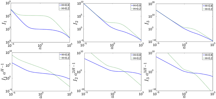
Figure 2. Top: Numerical computation of integrals I_k(a, L) defined in Equation (20) for two different Hurst exponents (plain line: H = 0.8, dashed line: H = 0.2). The size is L = 2¹⁹ and the integral has been sample averaged over twenty realizations. The regime of interest, where non-trivial scaling will occur, is in the region of intermediate values of a. As the figure runs over 11 orders of magnitude in a, this region may seem narrow in the figures. Bottom: The integrals have been rescaled by a^kH−1 I_k(a, L) in order to bring out the scaling regions more clearly. The region where we see scaling according to Equation (42) now appears horizontal. We have chosen H = 0.8.

In the three upper panels, we show I_k(a, L) with k = 1, 2, and 3 for H = 0.2 and H = 0.8. For H = 0.2, kH is always less than 1, the second regime is thus independent of a and the top curves of Figure 2 for H = 0.2 (dotted lines) show a flat middle section. For H = 0.8, we have kH < 1 only for k = 1 whereas for k = 2 and 3, we have kH > 1, the two curves for H = 0.8 and k = 2 and 3 should not, thus, show a flat middle section; this is actually what is observed in Figure 2. In the lower three panels we show the rescaled integrals a^{kH − 1} I_k(a, L) for k = 1, 2, and 3. Equation (42) then predicts that the middle sections of the two curves corresponding to H = 0.8 k = 2 and 3 (values for which kH > 1) should be flat whereas those for H = 0.2 and (H = 0.8, k = 1) should not (in those cases we have kH < 1).

We now return to the series expansions of the relation between pressure drop ΔP and flow rate Q. We have introduced the length scale a* in Equation (18) and the expansion for small flow rates—hence, small a*—is given in Equation (19). Combining this expression with the assumption that Δ^H ≪ a ≪ L^H, we find

$\begin{array}{cc}\begin{array}{l}\Delta P=-2{\sigma }_c\text{sgn}(Q)[{\displaystyle \sum _{k=0}^{[(1-H)/H]}{a}_k}{(a^{*})}^k{L}^{1-(k+1)H}\\ +{\displaystyle \sum _{[(1-h)/H]+1}^{\infty }{a}_k}\frac{{(a^{*})}^k}{a^{(k+1)-1/H}}],\end{array}& (44)\end{array}$

where [·] is the floor function. Hence, for 1/2 < H < 1, only the k = 0 term scales with L. For 1/3 < H < 1/2, the k = 0 and k = 1 terms scale with L.

The k = 0 term in (44) is the threshold pressure. We therefore have that

$\begin{array}{cc}{P}_c\propto 2{\sigma }_c\{\begin{array}{ll}\frac{\Delta }{a}\hfill & \text{if }a\ll \Delta /L^H,\hfill \\ L^{1-H}\hfill & \text{if }\Delta /L^H\ll a\ll L^H,\hfill \\ \frac{L}{a}\hfill & \text{if }{L}^H\ll a.\hfill \end{array}& (45)\end{array}$

The first regime corresponds to the situation where the yield stress is controlled by the minimal aperture region. In that case, the pressure gradient is dominated by the pressure drop over this particular region of the length Δ. The second threshold corresponds to the limit where yield stress is controlled the full length of the rough channel; in that case the typical aperture is related the self-affine nature of aperture and scales with the length of the channel like L^H. The third asymptotic regime is a channel of length L with parallel walls separate by a distance a. Let us now consider the large |Q|—the large a*—expansion. By combining Equation (25) with the scaling of I_k(a, L), we find

$\begin{array}{cc}\begin{array}{l}\Delta P=-2{\sigma }_c\text{sgn}(Q)[\frac{12{(a^{*})}^2}{a^{3-1/H}}+\frac{3}{2}{L}^{1-H}\\ +{\displaystyle \sum _{k=2}^{\infty }\frac{b_k}{{(a^{*})}^{2k}}}{a}^{1/H}{L}^{(2k-1)H}],\end{array}& (46)\end{array}$

as long as H > 1/3.

The scaling seen in this section is subtle. The difficulty lies in the presence of the length scale a*. This length scale is not present when the flow is Newtonian. In that case, the expression for the pressure drop vs. flow rate is ¹

$\begin{array}{cc}\Delta P=-\mu Q{I}_3(a,L)=-\mu Q\{\begin{array}{l}\begin{array}{ll}\frac{\Delta }{a^3}\hfill & \text{if }a\ll {\Delta }^H,\hfill \\ \frac{L^{\max (1-3H,0)}}{a^{\max (3H-1,0)/H}}\hfill & \text{if }{\Delta }^H\ll a\ll L^H,\hfill \\ \frac{L}{a^3}\hfill & \text{if }{L}^H\ll a,\hfill \end{array}\hfill \end{array}& (47)\end{array}$

where μ the viscosity. Hence, there are three scaling regimes in this case [26].

5. A Truncated Series Expansion

We present in this section a truncation of the series expansions of the flow equation, which nevertheless retains very close to the exact expression over the entire range of aperture opening a. This series is considerably simpler than the exact solution.

We combine the two expansions (19) and (25) by splitting up the integrals I_k(a, L), defined in Equation (20),

$\begin{array}{cc}\begin{array}{l}{I}_k(a,L)=I_k(\text{}<a^{*},L)+I_k(\text{}>a^{*},L)\\ ={\displaystyle {\int }_{h(x)<a^{*}}\frac{dx}{h{(x)}^k}}+{\displaystyle {\int }_{h(x)>a^{*}}\frac{dx}{h{(x)}^k}}.\end{array}& (48)\end{array}$

We combine the expansions (19) and (25) and get

$\begin{array}{cc}\begin{array}{l}\Delta P=-2{\sigma }_c\text{sgn}(Q)[{\displaystyle \sum _{k=0}^{\infty }{a}_k}{(a^{*})}^k{I}_{k+1}(\text{}>a^{*},L)\\ +12{(a^{*})}^2{I}_3(\text{}<a^{*},L)+\frac{3}{2}{I}_1(\text{}<a^{*},L)\\ +{\displaystyle \sum _{k=2}^{\infty }\frac{b_k}{{(a^{*})}^{2k}}}{I}_{1-2k}(\text{}<a^{*},L)].\end{array}& (49)\end{array}$

We truncate the series at second order, finding

$\begin{array}{cc}\begin{array}{l}\Delta P=-2{\sigma }_c\text{sgn}(Q)[a_0{I}_1(\text{}>a^{*},L)a_1(a^{*})I_2(\text{}>a^{*},L)\\ +a_2{(a^{*})}^2{I}_3(\text{}>a^{*},L)+12{(a^{*})}^2{I}_3(\text{}<a^{*},L)\\ +\frac{3}{2}{I}_1(\text{}<a^{*},L)]\end{array}& (50)\end{array}$

$\begin{array}{cc}\begin{array}{l}=-\text{sgn}(Q)P_c-\text{sgn}(Q)[4\sqrt{D{\sigma }_c}{I}_2(\text{}>a^{*},L)|Q{|}^{1/2}\\ +\frac{16}{3}D{I}_3(\text{}>a^{*},L)+12D|Q|I_3(\text{}<a^{*},L)\\ +{\sigma }_c{I}_1(\text{}<a^{*},L)],\end{array}& (51)\end{array}$

where we have used I₁(< a*, L) + I₁(> a*, L) = I₁.

In Figure 3, we plot this approximation and compare it to the exact solution.

FIGURE 3

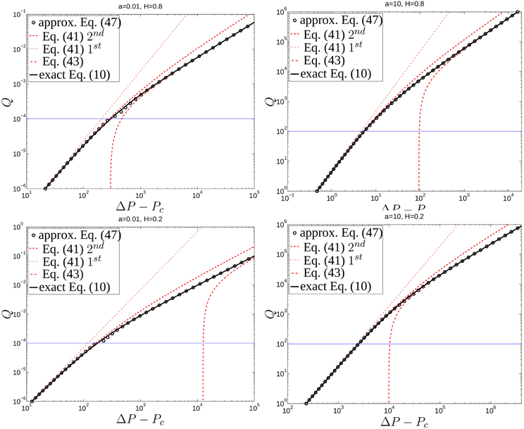
Figure 3. Flow rate Q as function of the applied pressure drop ΔP − P_c for different Hurst coefficient H and different openings a. The other parameters are D = 1/12, σ_c = 1, L = 2¹⁹. Black plain line represent numerical integration of the exact expression of Equation (12). Dashed lines represents the asymptotic regimes for Q ≪ 1 defined by Equation (44) (thick line: second order for thin line for first order) and for Q ≫ 1 defined by Equation (46) (first order). Open circles represent the combined asymptotic approximation Equation (50). The horizontal line, represents the flow rate at which a* = a, which represents the first decrease (resp. increase) of I_k(< a*, L) (resp. I_k(> a*, L). This flow rate corresponds also to the maximal error between the exact and approximated solution. This errors is respectively (from top-left to bottom-right): 10, 2, 12, and 5%.

The agreement with the analytical summation is very good for any opening and any Hurst coefficient. The reason for this good match can be understood as follows. At very low flow rate, if a* is smaller than any openings, we have then I_k(< a*, L) = 0 and I_k(> a*, L) = I_k(a, L). The combined expression is exactly equal to the expansion of Equation (44). As Q, one start to reach the point where a* = a (denoted as an horizontal line in Figure 3) which corresponds to the situation where the smallest element of the sum I_k(> a*, L) is removed but added in I_k(< a*). From there, all the integrals I_k(> a*, L) (respectively I_k(< a*, L)) are decreasing (respectively increasing) with Q until a* reaches the maximum opening. For this case, one then have I_k(> a*, L) = 0 and I_k(< a*, L) = I_k(a, L) and we recover the limiting case of Equation (46). The combined approximation allows us thus to match the two asymptotic limits of Equation (44) and (46).

This good agreement between the approximation and the exact solution let us to deduce sufficient condition of validity for the two expansions. Namely:

$\begin{array}{cc}\begin{array}{l}\text{If}{a}^{*}<\min \text{}(h)\Rightarrow \Delta P\simeq -\text{sgn}(Q)(2{\sigma }_c{I}_1(a,L)\\ +4I_2(a,L)\sqrt{{\sigma }_{c}D|Q|}+\frac{16}{3}{I}_3(a,L)DQ)\end{array}& (52)\end{array}$

$\begin{array}{cc}\begin{array}{l}\text{If}{a}^{*}>\max (h)\Rightarrow \Delta P\simeq -\text{sgn}(Q)(3{\sigma }_c{I}_1(a,L)\\ +12D{I}_3(a,L)|Q|).\end{array}& (53)\end{array}$

The validity of the regime reflects thus the heterogeneities of the aperture, particularly the two extremal values.

6. Conclusion

In this work, we have investigated the flow rate in a 1D rough channel for any aperture distribution. We have, however, paid particular attention to the case of aperture fields that are self affine, which is e.g., the case when the aperture field is given by the channel being a fracture.

Our first result is given in Equation (12). This gives the total flow rate Q as a function of pressure difference ΔP across the length of the channel. Whatever the geometry of the channel, close to the pressure threshold P_c, the flow rate scales like (ΔP − P_c)² with a prefactor function of the fluid and aperture properties. We have introduced a characteristic length scale a* = $\sqrt{\frac{DQ}{2{\sigma }_c}}$ where the square root scaling is a direct consequence of the square variation of the flow rate with the pressure. The length scales a* allows an expansion in series of the two limit cases, the low (a* < a) and high (a* > a) flow rates regimes where a is the minimal aperture. At large flow rate (large a*), the flow rate scales linearly as (ΔP − $\frac{3}{2}$P_c), with an apparent critical pressure $\frac{3}{2}$P_c larger than the actual one P_c.

With this length scale, we combine the series expansions and truncate them in a way that leads to high accuracy. The sum of the two contributions is found to provide a good approximation for the exact solution given by Equation (12) in the case of self-affine channels.

One of the main consequences of this results is the fact that, in principle, one should expect four different flowing regimes in porous media. Presently, only three flowing regimes have been observed numerically (see [15]). The first one, in the limit ΔP ~ P_c, is linear ( i.e., Q ~ (ΔP − P_c)) and corresponds the flow channelization along one channel. Here we have demonstrate that, in addition to this regime, one should observed another quadratic regime where Q ~ (ΔP − P_c)². As a consequence, by increasing the pressure, one should observes regimes in the following sequence: quadratic (one channel), linear (one channel), quadratic (with an increase of channels) and linear (when all channels are open).

It is important to recall that this work is only valid under the lubrication limit. Lubrication approximations have been investigated extensively for Newtonian fluids in confined geometries (e.g., [32, 33]). For visco-plastic fluids, the limit of lubrication has also been investigated by various authors in different geometries (see [34] for film flows, [22–24, 35] for confined geometries and [36, 37] for experiments). In this case, the lubrication hypothesis becomes very restrictive essentially due to rigidity of the plug regions. As discussed above (and in details by Frigaard and Ryan [23]), because of the aperture variations and the mass conservation, lubrication approximation leads to variations of the plug velocity. However, such variations are forbidden in the case of ideal visco-plastic fluids which prevent any extensional deformations. Consequently, one expects deviations from the lubrication hypothesis as the amplitude of the variations becomes important.

As for flow in channels with self-affine aperture fields, we do not find a simple scaling law for the equivalent of the permeability as was the case for newtonian fluids [26]. Rather, we find the each term in the series expansions of the flow equation scales with its own scaling exponent in the aperture opening a. By combining these results with the truncated series given in section 5, it is tractable how the flow equations evolve with varying a in this case.

Future work will be dedicated to the investigation of the validity conditions of our analytical expressions. We have not considered two and three-dimensional channels. As for the case of Newtonian flow, this is much more complex than the present case. However, as was remarked in the Introduction, at small pressure gradients, the flow will be confined to single channels, i.e., the precise situation considered in the present paper.

Conflict of Interest Statement

The authors declare that the research was conducted in the absence of any commercial or financial relationships that could be construed as a potential conflict of interest.

Acknowledgments

The authors would like to thank J. P. Hulin, S. Roux, and D. Salin for interesting for useful discussions, the “Agence National de la Recherche” for financial support of the project LaboCothep ANR-12-MONU-0011.

Footnotes

1. ^In [26], the case when H < 1/3 was not discussed in connection with Equation (42) for k = 3.

References

1. Bingham E. The behavior of plastic materials. Bulletin of US bureau of standards. (1916) 13:309–53.

2. Chevalier T, Chevalier C, Clain X, Dupla JC, Canou J, Rodts S, et al. Darcy's law for yield stress fluid flowing through a porous medium. J Non-Newtonian Fluid Mech. (2013) 195:57–66. doi: 10.1016/j.jnnfm.2012.12.005

CrossRef Full Text

3. Wu YS, Pruess K, Witherspoon PA. Displacement of a Newtonian fluid by a non-Newtonian fluid in a porous medium. Trans Porous Media (1991) 6:115–42. doi: 10.1007/BF00179276

CrossRef Full Text

4. Wu Y, Pruess K, Witherspoon P. Flow and displacement in Bingham non-Newtonian fluids in porous media. SPE Res Eng. (1992) 7:369–76. doi: 10.2118/20051-PA

CrossRef Full Text

5. Barenblatt GI, Entov VM, Ryzhik VM. Theory of Fluid Flows Through Natural Rocks. Norwell, MA: Kluwer Academic Publishers (1989).

6. Rossen WR. Foams in enhanced oil recovery. In: Prudhomme RK, Khan S, editors. Foams: Theory, Measurements and Applications. New York, NY: Marcel Dekker (1995). 414–63.

7. Wang D, Cheng J, Yang Q, W Gong QL, Chen F. SPE. Presented at the 2000 SPE Annual Technical Conference and Exhibition Held in Dallas, Texas (2000) 63227.

8. Choi SK, Ermel YM, Bryant SL, Huh C, Sharma MM. Transport of a pH-Sensitive polymer in porous media for novel mobility-control applications. Soc Petrol Eng. (2006) 99656. doi: 10.2118/99656-MS

CrossRef Full Text

9. Chevalier T, Rodts S, Chateau X, Chevalier C, Coussot P. Breaking of non-Newtonian character in flows through a porous medium. Phys Rev E (2014) 89:023002. doi: 10.1103/PhysRevE.89.023002

CrossRef Full Text

10. Balhoff MT, Thompson KE. Modeling the steady flow of yield-stress fluids in packed beds. AICHE J. (2004) 50:3034–48. doi: 10.1002/aic.10234

CrossRef Full Text

11. Chen M, Rossen W, Yortsos YC. The flow and displacement in porous media of fluids with yield stress. Chem Eng Sci. (2005) 60:4183–202. doi: 10.1016/j.ces.2005.02.054

CrossRef Full Text

12. Sochi T, Blunt MJ. Pore-scale network modeling of Ellis and Herschel-Bulkley fluids. J Petrol Sci Eng. (2008) 60:105–24. doi: 10.1016/j.petrol.2007.05.009

CrossRef Full Text

13. Morais AF, Seybold H, Herrmann HJ, Andrade JS. Non-Newtonian fluid flow through three-dimensional disordered porous media. Phys Rev Lett. (2009) 103:194502. doi: 10.1103/PhysRevLett.103.194502

Pubmed Abstract | Pubmed Full Text | CrossRef Full Text

14. Sochi T. Non-Newtonian flow in porous media. Polymer (2010) 51:5007–23. doi: 10.1016/j.polymer.2010.07.047

CrossRef Full Text

15. Talon L, Bauer D. On the determination of a generalized Darcy equation for yield-stress fluid in porous media using a Lattice-Boltzmann TRT scheme. Eur Phys J E (2013) 36:1–10. doi: 10.1140/epje/i2013-13139-3

Pubmed Abstract | Pubmed Full Text | CrossRef Full Text

16. Balhoff M, Sanchez-Rivera D, Kwok A, Mehmani Y, Prodanović, M. Numerical algorithms for network modeling of yield stress and other non-Newtonian fluids in porous media. Trans. Porous Media (2012) 93:363–79.

17. Roux S, Herrmann HJ. Disorder-induced nonlinear conductivity. Eur Lett. (1987) 4:1227. doi: 10.1209/0295-5075/4/11/003

CrossRef Full Text

18. Chaplain V, Mills P, Guiffant G, Cerasi P. Model for the flow of a yield fluid through a porous medium. J Phys II (1992) 2:2145–58. doi: 10.1051/jp2:199225.

CrossRef Full Text

19. Al-Fariss T, Pinder KL. Flow through porous media of a shear-thinning liquid with yield stress. Can J Chem Eng. (1987) 65:391–405. doi: 10.1002/cjce.5450650306

CrossRef Full Text

20. Sinha S, Hansen A. Effective rheology of immiscible two-phase flow in porous media. Eur Lett. (2012) 99:44004. doi: 10.1209/0295-5075/99/44004

CrossRef Full Text

21. Talon L, Auradou H, Pessel M, Hansen A. Geometry of optimal path hierarchies. Eur Lett. (2013) 103:30003. doi: 10.1209/0295-5075/103/30003

CrossRef Full Text

22. Putz A, Frigaard IA, Martinez DM. On the lubrication paradox and the use of regularisation methods for lubrication flows. J Non-Newtonian Fluid Mech. (2009) 163:62–77. doi: 10.1016/j.jnnfm.2009.06.006

CrossRef Full Text

23. Frigaard IA, Ryan DP. Flow of a visco-plastic fluid in a channel of slowly varying width. J Non-Newtonian Fluid Mech. (2004) 123:67–83. doi: 10.1016/j.jnnfm.2004.06.011

CrossRef Full Text

24. Roustaei A, Frigaard IA. The occurrence of fouling layers in the flow of a yield stress fluid along a wavy-walled channel. J Non-Newtonian Fluid Mech. (2013) 198:109–24. doi: 10.1016/j.jnnfm.2013.03.005

CrossRef Full Text

25. Oron A, Davis SH, Bankoff SG. Long-scale evolution of thin liquid films. Rev Mod Phys. (1997) 69:931. doi: 10.1103/RevModPhys.69.931

CrossRef Full Text

26. Talon L, Auradou H, Hansen A. Permeability of self-affine aperture fields. Phys Rev E (2010) 82:046108. doi: 10.1103/PhysRevE.82.046108

Pubmed Abstract | Pubmed Full Text | CrossRef Full Text

27. Mandelbrot BB, Passoja DE, Paullay AJ. Fractal character of fracture surfaces of metals. Nature (1984) 308:721–2. doi: 10.1038/308721a0

CrossRef Full Text

28. Bouchaud E, Lapasset G, Planes J. Fractal dimension of fractured surfaces - a universal value. Eur Lett. (1990) 13:73–9. doi: 10.1209/0295-5075/13/1/013

CrossRef Full Text

29. Måløy KJ, Hansen A, Hinrichsen EL, Roux S. Experimental measurements of the roughness of brittle cracks. Phys Rev Lett. (1992) 68:213. doi: 10.1103/PhysRevLett.68.213

Pubmed Abstract | Pubmed Full Text | CrossRef Full Text

30. Bonamy D, Bouchaud E. Failure of heterogeneous materials: a dynamic phase transition? Phys Rep. (2011) 498:1–44. doi: 10.1016/j.physrep.2010.07.006

Pubmed Abstract | Pubmed Full Text | CrossRef Full Text

31. Guyon E, Hulin JP, Petit L. Hydrodynamique Physique. Les Ulis: EDP sciences (2001).

32. Reynolds O. On the theory of lubrication and its application to Mr. beauchamp tower's experiments, including an experimental determination of the viscosity of olive oil. Philos Trans R Soc Lond B Biol Sci. (1886) 177:157–234.

33. Dowson D. A generalized Reynolds equation for fluid-film lubrication. Int J Mech Sci. (1962) 4:159–70. doi: 10.1016/S0020-7403(62)80038-1

CrossRef Full Text

34. Balmforth NJ, Craster RV. A consistent thin-layer theory for Bingham plastics. J Non-Newtonian Fluid Mech. (1999) 84:65–81. doi: 10.1016/S0377-0257(98)00133-5

CrossRef Full Text

35. Walton IC, Bittleston SH. The axial flow of a Bingham plastic in a narrow eccentric annulus. J Fluid Mech. (1991) 222:39–60. doi: 10.1017/S002211209100099X

CrossRef Full Text

36. de Souza Mendes PR, Naccache MF, Varges PR, Marchesini FH. Flow of viscoplastic liquids through axisymmetric expansions contractions. J Non-Newtonian Fluid Mech. (2007) 142:207–17. doi: 10.1016/j.jnnfm.2006.09.007

CrossRef Full Text

37. Chevalier T, Rodts S, Chateau X, Boujlel J, Maillard M, Coussot P. Boundary layer (shear-band) in frustrated viscoplastic flows. Europhys Lett. (2013) 102:48002. doi: 10.1209/0295-5075/102/48002

CrossRef Full Text