Robust super-resolution by fusion of interpolated frames for color and grayscale images

Introduction

Commercial visible color cameras using a single focal plane array (FPA) will typically use a CFA to collect red, green, and blue (RGB) spectral scene information. While there are many proposed color arrangements for CFAs [1], the Bayer pattern remains the most widely used [2]. The Bayer pattern is a repeating 2 × 2 filter where the green filter is in a quincunx arrangement with twice the sampling density of the red and blue filters. Only one color channel is collected in each spatial sample. The other two bands must be estimated. Extensive research has gone into this demosaicing process [3–5]. Additionally, grayscale cameras will typically balance sampling with other factors, such as signal-to-noise ratio (SNR). This generally results in undersampled, aliased images [6]. Because CFA cameras trade spatial sampling for color information, aliasing issues are exacerbated.

Multi-frame super-resolution (SR) is an effective method for reducing aliasing in images that are limited by detector sampling. Motion between image frames increases sampling diversity. By combining image samples from multiple low resolution (LR) frames into a single high resolution (HR) image, aliasing can be reduced or eliminated. A thorough SR overview is provided in [7] and a compendium of recent research is contained in [8]. Many SR methods utilize iterative approaches. These variational approaches tend to be computationally intensive and may not be amenable to real-time implementation. Another approach, based on non-uniform interpolation, tends to be computationally simpler than variational methods. These methods can provide fast, potentially real-time implementation. The approach is to notionally place all accurately registered frame samples into a common HR space. If uncontrolled inter-frame motion is present, this results in non-uniform sampling. The non-uniformly sampled data is used to interpolate onto a uniform HR grid and restoration can then be applied. The fast adaptive Wiener filter (AWF) combines interpolation and restoration simultaneously in a spatially-adaptive weighted sum [9]. The AWF approach allows restoration to be optimized for specific local non-uniform spatial arrangements on the HR grid. For strictly translational motion, it is possible to pre-compute all the AWF filter weights since the observed pixel spatial pattern on the HR space is periodic. Therefore, the number of filter weights is small, further increasing computational speed. For affine inter-frame motion, the full set of AWF weights is generally impractical to pre-compute. A previously developed AWF SR method for affine motion [10] places LR data onto a discrete grid rather than continuous HR space and uses a partial observation window. Under these conditions, filter weights can be pre-computed. However, quantization onto a discrete grid can increase registration errors, impacting SR performance [11]. Thus, treating affine inter-frame motion using fast algorithms remains a challenge for SR.

Multi-frame SR in scenes that include small moving objects can also be a challenge. Adding local motion robustness has recently received attention [12–20]. Much of the research utilizes iterative methods with increased computational complexity. AWF SR was extended to add local motion robustness [21]. Beginning with a parametric global motion model, data that are inconsistent with the global motion model are excluded from contributing to the multi-frame AWF output. Areas of local motion are handled separately with a single frame AWF SR filter.

Color multi-frame SR for CFA cameras is another area of recent research and it can be viewed as an SR extension to demosaicing. Many documented methods implement variational approaches. These primarily differ in the implementation of the data fidelity and/or regularization terms [22–29]. An AWF SR method for CFA color imagery was proposed [11]. This approach employs parametric correlation and color cross-correlation models to utilize cross-channel data and improve SR results over independent channel SR methods. The approach was implemented for translation-only global inter-frame motion. This constraint allowed observed data samples to be placed onto a continuous HR space and not be quantized to a discrete HR grid.

In this paper, we propose an SR method that we believe addresses many of the practical issues raised above, while maintaining a relatively low computational complexity. We refer to the new method as Fusion of Interpolated Frames (FIF) SR. The FIF method has been designed to simplify SR for CFA sensors when the inter-frame motion is more complex than simple translation. However, the approach can be applied to standard single channel imaging sensors as well. To provide computational simplicity, FIF SR decouples the demosaicing, interpolation, and restoration steps in the SR process. After demosaicing and single frame interpolation/registration, FIF SR uses a novel weighted sum of the interpolated full-color frames for an improved HR estimate. There are three components to the weight: a subpixel interpolation distance metric, a motion model error metric, and an estimate of channel cross-correlation. Finally, restoration is applied to deconvolve the system point spread function (PSF). We show that FIF can handle affine inter-frame motion with robustness to locally moving small objects. These motion conditions are typical in airborne imaging applications [21]. As far as we are aware, this approach is unique and has not been investigated previously.

The rest of the paper is organized as follows. In Section Observation and Reconstruction Models, we present the observation model used to form the basis of the reconstruction approach. We provide details of the FIF SR algorithm for Bayer CFA data in Section FIF SR Algorithm. Experimental results using both simulated and real data sets with varying levels of imaging complexity are provided in Section Experimental Results. Finally, we provide conclusions in Section Conclusion.

Observation and Reconstruction Models

A forward observation model is used to develop the FIF SR method. The model relates the true wavelength-dependent continuous scene to observed low resolution (LR) images. We employ the alternative observation model of [11], shown in Figure 1. This model commutes inter-frame motion and the system PSF relative to the order of operations in a physical system. This commutation holds true for translational motion and a spatially invariant PSF. It also holds true for rotational motion if the PSF is circularly symmetric, and approximately for full affine motion if zoom and shear are limited [10]. The continuous scene d(x, y, λ) is imaged by a system with camera motion between frames. Spectral channel filters are applied, creating J continuous images. For Bayer cameras, the channel filters are 3 spectral filters. The color channels, red, green, and blue (RGB), can be represented by j = 1, 2, and 3, respectively. The output is degraded by the system PSF, represented by h_j(x, y), where j designates a unique wavelength-dependent PSF for each channel. Camera motion results in a geometric transformation of d(x, y, λ). The variable α_p captures global inter-frame motion parameters for all frames, p = 1, 2, …, P. The filtered continuous outputs are sampled according to the detector array CFA pattern, creating the lexicographical vectors f(p). Finally, n(p) are vectors of additive noise samples. The noise samples are assumed to be zero-mean independent and identically distributed Gaussian random variables with a variance of σ²_η. The observed frames are then represented as g(p) = f(p) + n(p). For a Bayer CFA camera, these observed frames can be represented as g(p) = [g₁(p)^T, g₂(p)^T, g₃(p)^T]^T, where g₁(p), g₂(p), and g₃(p) correspond to the color channels. The ideally sampled image is represented in lexicographical form by the vector z = [z^T₁, z^T₂, z^T₃]^T, where z_j = [z_{j, 1}, z_{j, 2}, …, z_{j, MN}]^T contains the ideal samples for channel j. The parameters M, N are the number of desired HR samples in the x, y directions, respectively, to achieve Nyquist sampling.

FIGURE 1

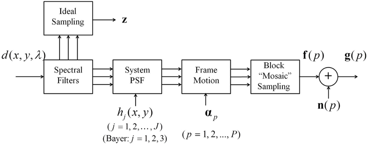
Figure 1. Forward observation model used to develop the FIF SR method.

The system PSF can account for a number of imaging system effects. For this work, we follow the approach in [11] and include only optical diffraction and spatial detector integration. For a diffraction-limited optical system, the spatial cutoff frequency is given by

$\begin{array}{cc}{\rho }_c=\frac{1}{\lambda f/\#}(\text{cyc}/\text{mm}),& (1)\end{array}$

where λ is the center wavelength of light into the system and f / # is the optical f-number. According to the Nyquist Sampling Theorem [30], a band-limited image can be uniquely determined from its discrete samples if it is sampled at twice or more than the cutoff frequency,

$\begin{array}{cc}\frac{1}{{\delta }_s}\ge 2{\rho }_c.& (2)\end{array}$

Here, δ_s is the spatial sampling interval (i.e., pixel pitch) and 1/δ_s is the spatial sampling frequency. For a single color of the Bayer CFA image, the spatial sampling is based on the detector pitch and CFA pattern. The CFA doubles detector sampling interval for red and blue color filters (approximately 1.4× for the quincunx-sampled green filter), leading generally to increased aliasing over panchromatic cameras of the same fundamental detector pitch.

FIF SR algorithm

A block diagram of the FIF SR algorithm is illustrated in Figure 2. The major steps in the FIF are demosaicing (for CFA input imagery only), registration and interpolation, fusion of interpolated frames, and restoration. Figure 3 shows an output image at major steps to illustrate the dimensionality and information produced by each of these steps. Note that the desired HR sampling grid is designated by the upsampling factor parameter L, which represents the ratio of desired full-color HR sampling to basic CFA sampling of the red (or blue) color channels. Figure 3 shows each input CFA image of size 192 × 128, so the red (or blue) channel size is 96 × 64. Applying SR to the level of L = 8 results in the desired full-color image of size 768 × 512. The following subsections address each of the major algorithm steps in detail.

FIGURE 2

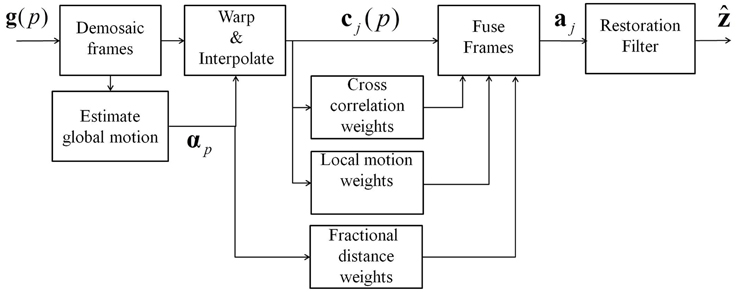
Figure 2. Overview of the FIF SR method.

FIGURE 3

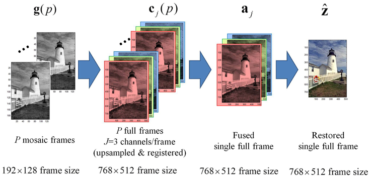
Figure 3. Graphical details of major steps in FIF process.

Demosaicing

The first step is to demosaic the observed CFA image set, recovering the full-color image at each temporal frame. Note that in the case of grayscale imagery, this step is simply bypassed. Extensive research has been done on demosaicing Bayer images and much has focused on reducing interpolation artifacts with edge adaptive techniques or color channel cross-correlation. For FIF SR, one may choose any suitable method for the type of data involved. Here we use a gradient-corrected bilinear interpolation method with gains to control the level of correction [31]. With fixed gain coefficients, this method can be implemented with a set of finite impulse response (FIR) filters to increase speed. This is accomplished with a set of simple 5 × 5 linear filters with 9 coefficients for the green channel and 11 coefficients for each of the blue and red channels. Because each channel filter is independent, the channels can be filtered in parallel.

Registration and Interpolation

With the full-color LR image set now available, the next steps are to register and interpolate the images to a common reference grid at the desired SR sampling resolution. This process results in a set of P full-size color images, sampled at the desired output M × N HR level. As shown in Figure 2, this image set is designated as c_j(p) = [c_{j, 1}(p), c_{j, 2}(p), …, c_{j, MN}(p)]^T, for channel j = 1, 2, …, J and frame p = 1, 2, …, P.

In this work, we assume that global background motion is dominant. Global affine parameters are estimated for each frame relative to the selected reference frame (usually the most recent frame). These affine parameters are estimated using an iterative gradient-based least squares algorithm [32] at multiple scales [33]. This approach is described in [10], with analyses of aliasing impacts shown in [21]. For general J channel data, parameters can be estimated for each demosaiced channel data and then averaged. For the Bayer CFA, we use the demosaiced green channel data to estimate the motion parameters. Because the green channel is more densely sampled in the observed CFA data, the demosaiced green channel data generally contains less aliasing than the red or blue channels. This results in better registration estimates. To further reduce aliasing impacts for motion parameter estimation, the images are pre-filtered with a Gaussian low pass filter (LPF). Finally, to improve motion parameter estimation when local moving objects are present, a fraction of the highest motion error pixels that don't obey the global motion assumption are excluded using the approach of [21].

With the registration parameters now estimated, each of the demosaiced frames can be interpolated and aligned to the HR reference grid by means of a global affine warping. In our implementation, we first resize the demosaiced images with a Lanczos kernel interpolator to get the images to the HR size (or higher), and then apply the affine warping the images using simple bilinear interpolation. The Lanczos kernel is a sinc windowed sinc function and is considered to represent a good compromise between complexity and upsampling performance [34]. It can be implemented efficiently using fast Fourier Transform filtering. Using bilinear interpolation on the Lanczos resized images provides the necessary affine warping with a low computational complexity. The Lanczos resizing prior to bilinear interpolation means that the bilinear interpolation has a finer grid to start from, and its deficiencies are minimized. One can, of course, implement the warping and resizing in one step, provided you sacrifice Lanczos performance or bilinear interpolation speed.

The most complex operation in this step is multi-scale affine motion estimation. This operation is simplified by using a single channel for the estimation. Each frame is registered independently, so the estimation can be implemented as a parallel operation. The actual upsampling and warping are also performed independently by channel and frame, so those steps can also be parallelized.

Fusion of Interpolated Frames

The heart of the FIF SR method is the fusion of the interpolated frames from the previous step. The result is a single HR image for each channel, denoted a_j = [a_{j, 1}, a_{j, 2}, …, a_{j, MN}]^T for j = 1, 2, … J. The fusion is done by means of a weighted sum of the input frames. In particular, each output pixel is a weighted sum of all of the corresponding pixels at the same spatial location from the interpolated input channels frames. This weighted sum is given by

$\begin{array}{cc}{a}_{j,k}=\frac{{\displaystyle \sum _{p=1}^P{\displaystyle \sum _{q=1}^3{w}_{j,k}}}(q,p)·c_{q,k}(p)}{{\displaystyle \sum _{p=1}^P{\displaystyle \sum _{q=1}^3{w}_{j,k}}}(q,p)},& (3)\end{array}$

for j = 1, 2, …, J and k = 1, 2, …, MN. Note that a_{j, k} is spatial sample k of channel j in the fused image, and w_{j, k} (q, p) is the weight for the q^th color channel of the p^th frame at spatial location k used to estimate a_{j, k}. A special case of the FIF algorithm is when the fusion does not use color cross-channel information in estimating a given HR image channel. Each channel a_{j, k} is estimated using only data from its own color channel and spatial location. The normalized weighted sum for this simpler “independent channel” FIF SR is

$\begin{array}{cc}{a}_{j,k}=\frac{{\displaystyle \sum _{p=1}^P{w}_{j,k}}(j,p)·c_{j,k}(p)}{{\displaystyle \sum _{p=1}^P{w}_{j,k}}(j,p)},& (4)\end{array}$

for j = 1, 2, …, J and k = 1, 2, …, MN. These weighted summations are sample-based calculation, so every fused sample and channel can be calculated in parallel.

To understand the rationale of our approach to defining the fusion weights, it may be helpful to consider that each interpolated frame can be viewed as a noisy and blurred realization of the true image z. In addition to traditional sensor noise, demosaicing and interpolation error in these images, resulting from aliasing, can be viewed as a noise source that will vary from frame to frame because of inter-frame motion. Local motion can also be viewed as a “noise” relative to the ideal reference image. In light of this, the fusion step uses a weighted sum of all interpolated frames at the k^th spatial position to estimate the k^th HR output pixel in each channel. The weights we propose have three components. The first component seeks to deemphasize interpolated pixels with a large demosaicing and interpolation error, in favor of those with less. The second seeks to deemphasize pixels where the local motion departs from the reference frame, in favor of those that match the reference. Finally, the third component seeks to exploit inter-channel correlation. Let the weight components be defined as follows

$\begin{array}{cc}{w}_{j,k}(q,p)=w_k^{(1)}(q,p)·w_k^{(2)}(p)·w_{j,k}^{(3)}(q).& (5)\end{array}$

Calculating the weight for each channel and sample is a sample-based calculation. Every sample and channel can be calculated in parallel. Each weight component is described in detail in the following subsections.

Interpolation Error Weight

The first weight, w⁽¹⁾_k(q, p), captures information regarding the interpolation error associated with c_{q, k}(p). This weight is inversely proportional to the fractional LR pixel distance between HR spatial position k and the nearest original LR observed pixel from g_q(p) (LR frame p channel q) without interpolation. The idea being that if an original LR pixel from LR frame p channel q is very close spatially to HR position k, we can expect less interpolation error in c_{q, k}(p). Thus, we wish to have increased weight for that sample [i.e., increased w⁽¹⁾_k(q, p)]. Based on the registration information, the coordinates of each LR observed pixel can be expressed in terms of the HR grid, in order to facilitate the pixel distance calculations.

Let R_k(q, p) represent the Euclidean distance (expressed in LR pixel spacing) between HR spatial position k and the nearest original LR observed pixel from g_q(p). When R_k(q, p) = 0, we wish to have a weight of w⁽¹⁾_k(q, p) = 1, and this represents the case where there is no demosaicing/interpolation error. As R_k(q, p) increases, we wish to have w⁽¹⁾_k(q, p) decrease. Multiple robust loss functions, used for M-estimation and denoising applications [35], were investigated for potential use in developing the weight function. An experimental study was performed in which the entire FIF algorithm was implemented and multiple robust loss functions were assessed in the weight component calculations. In this application, we have achieved good results using a robust Leclerc loss function. This function has a similar form to a Gaussian function and is expressed as

$\begin{array}{cc}{w}_k^{(1)}(q,p)=exp\left(\frac{-R_k{(q,p)}^2}{2h_s^2}\right),& (6)\end{array}$

where h_s is a tuning parameter for the rate of decay with fractional distance. Since the calculation of each w⁽¹⁾_k(q, p) value is independent, this operation can be performed in parallel for each sample and channel.

We see that, at zero fractional distance, the weight will have a value of 1. At large fractional distances, the weight approaches zero. Figure 4 shows an example of this concept for a single color channel, q = 1 (red channel), and frame p with SR at the L = 2 level. For HR sample k = 6, the nearest LR sample from observed LR red channel has a relatively large distance of R₆(1, p), as shown. On the other hand, HR sample k = 9, has a small distance of R₉(1, p). Thus, we expect that c_1,9(p) will have less interpolation error than c_1,6(p). The weights will exploit this information by means of Equation (6).

FIGURE 4

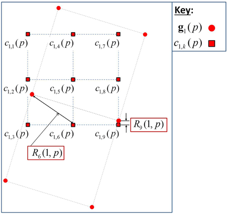
Figure 4. Single frame example showing the basis for fractional distance measurements.

Local Motion Weight

Local motion is determined by calculating the difference between each frame and the reference frame in c_q(p). Because c_q(p) still contains aliasing, simple differencing will induce extraneous errors since aliased regions can appear as local motion. Therefore, an LPF is applied prior to calculating the difference frames [21]. Implicit in this step is the assumption that local motion is due to extended objects moving between frames. This requires filtering at a level to sufficiently reduce aliasing artifacts while maintaining the ability to locate moving objects [21]. A small kernel maximum filter is applied after the LPF to maintain the integrity of small, extended moving objects (as small as 3–5 pixels).

Note that if local motion is present, it may impact every color channel in c_q(p). As with registration, we use the green channel of CFA imagery to estimate the local motion because of the reduced aliasing in this channel. If a pixel is impacted by local motion, we wish to reduce the weight associated with this sample in the weighted sum. We found good results using the robust Leclerc function as

$\begin{array}{cc}{w}_k^{(2)}(p)=exp\left(\frac{-D_k^2(p)}{2h_m^2}\right),& (7)\end{array}$

where D_k(p) is the LPF difference frame value at sample k of frame p relative to the reference frame. The term h_m is a tuning parameter that controls the sensitivity of the function to the difference values. Note that the reference frame pixel at each location will also get a local motion weight of 1. The weight is a sample-by-sample calculation based on frame differencing. Therefore, each sample can be independently calculated in parallel.

Channel Cross-Correlation Weight

Full-color images can have regions of high color cross-correlation. This cross-correlation can be leveraged in FIF so that all q colors in c_q(p) can be used to estimate every j HR channel. The channel cross-correlation weight captures this spatially-varying color cross-correlation. Through assessing multiple robust functions, the best performance has been found using a modified bisquare robust function [35] as

$\begin{array}{cc}{w}_{j,k}^{(3)}(q)=\{\begin{array}{cc}{\left[1-\frac{S_k^2}{h_c^2}\right]}^8& S_k<h_c\text{and}j\ne q\\ 0& S_k\ge h_c\text{and}j\ne q\\ 1& j=q\end{array}.& (8)\end{array}$

The term h_c is a tuning parameter and S_k is an estimate of the color saturation at HR sample k. This function has a value of 1 when there is zero saturation and has a value of zero when saturation is large. When the output and input color channels match (i.e., j = q), this gives a weight of 1. For cross-channels, if the saturation is above the threshold of h_c, the non-matching input color channel gets a weight of 0 and is therefore not used at all. In non-saturated regions, the non-matching input color is given a non-zero weight.

The premise for using color saturation follows from prior work in demosaicing and SR. Many SR methods for CFA images incorporate some aspect of color cross-correlation [11, 25, 36, 37]. Additionally, many demosaic methods use smooth hue transition assumptions in the form of color ratios or color differences [38–42]. These approaches recognize the benefit of utilizing color correlation to improve algorithm performance. We use the color saturation channel from the hue, saturation, value (HSV) color space hexcone model [43] which is functionally related to color ratios and differences.

Using the color saturation channel as a spatially-varying metric for assessing color correlation seems reasonable. For example, a pure grayscale region has highly correlated color channels. These regions also completely lack color saturation, so there appears to be a functional relationship between saturation of cross-correlation. In image regions completely saturated by a single color, using a large cross-channel weight would introduce noise artifacts into this channel because of noise in low-valued color channels. Here, better SR results may be achieved by applying a small cross-correlation weight and using only the saturated color channel [44].

The challenge now is to estimate the saturation values on the HR grid in the presence of sensor noise, aliasing, and local motion. To reduce aliasing, an LPF is applied to every frame of c_j(p). The resulting image set is designated as the local mean image set ĉ_j(p) = [ĉ_{j, 1}(p), ĉ_{j, 2}(p), …ĉ_{j, MN}(p)]^T. Because regions of location motion will negatively impact the calculation, we use the local motion weight w⁽²⁾_k(p) and form a robust local mean image as follow

$\begin{array}{cc}{\overline{c}}_{j,k}=\frac{{\displaystyle {\sum }_{p=1}^P{w}_k^{(2)}}(p){\widehat{c}}_{j,k}(p)}{{\displaystyle {\sum }_{p=1}^P{w}_k^{(2)}}(p)},& (9)\end{array}$

where c_j = [c_{j, 1}, c_{j, 2}, …, c_{j, MN}]^T. The color saturation values are computed from these local mean images using the hexcone model [43]. The weight in Equation (8) and the saturation channel are sample-based operations, so these steps can be implemented in parallel by sample. Creating the local mean image requires a filtering operation, but the weighted sum in Equation (9) is sample-based and can be implemented in parallel.

Restoration Filter

The FIF SR estimate, ẑ, is completed by applying a Wiener filter to the fused image channel image, a_j. We use a fast Fourier transform (FFT) based Wiener filter with constant noise to signal ratio parameter, Γ[45]. A wavelength-dependent restoration filter is applied to each channel. The restoration is quite straightforward and fast, requiring only an FFT, multiplication, and inverse FFT.

The Wiener filter is the minimum mean square error estimator for wide-sense stationary and Gaussian signals and noise [46]. It may not be optimal in other cases. For example, it is known to have difficulty dealing with highly non-Gaussian noise, such as impulsive noise. Notwithstanding this, it is a very widely used image restoration method, blending noise smoothing and inverse filtering [46]. We believe it provides a practical and useful solution this application. It offers a good balance between computational complexity and performance. Note that other restoration methods could be employed at this stage in the FIF algorithm as required by the signal and noise statistics.

Experimental Results

Experimental results are presented here to demonstrate the efficacy of the FIF SR approach. We begin with simulated data experiments that allow us to quantify performance. Results from real datasets are also presented. Real data experiments include Bayer CFA data and panchromatic data. The panchromatic data is from an airborne midwave infrared (MWIR) sensor system. The FIF SR algorithm is compared with multiple SR approaches. The most fundamental method is to simply demosaic the single-frame reference LR image and interpolate the result to the desired HR image size. We use the MATLAB “demosaic” function and cubic spline interpolation for this method.

We also include the color AWF SR method of [11]. The color AWF SR algorithm follows the full 12-parameter, 3-PSF model. A variational method using regularized least squares (RLS) is also included. This is a multi-channel extension to the method of [47]. The RLS is modified to perform independent-channel SR on Bayer images. We also present results of the SR method described in [25]. This method, called Multi-Dimensional Signal Processing (MDSP), is a maximum a posteriori (MAP) approach.

The above SR methods were developed specifically for global translational-only motion and do not accommodate local motion scene objects. For experiments containing global affine motion with local motion, we include a modified version of RLS, termed “robust” RLS. Affine motion estimation is implemented in a manner similar to [21]. Local motion detection is included and the single reference frame is applied in locations of detected motion in any of the input frames. The robust RLS method has been modified to handle data from Bayer CFA cameras and SR is performed independently on each channel. For these more complicated imaging conditions, the translation-only color AWF SR method was also modified to handle local motion. Single frame color AWF SR is performed in regions where local motion is detected.

Quantitative metrics used for the simulation experiments include mean square error (MSE) and mean absolute error (MAE). These two metrics are typically used in quantitative comparisons. However, these metrics may not necessarily correlate to visual perception of image quality. To provide alternate quantitative metrics, we also include the Multi-Scale Structural Similarity (MS-SSIM) Index [48]. MS-SSIM was developed for grayscale images. For color image comparisons, MS-SSIM is calculated on each channel separately. Feature, Similarity Index (FSIM) [49] is also used. This metric captures low-level features, primarily toward the local structure. A color extension to FSIM (called FSIMc) was developed by incorporating luminance and chrominance components. The scale for MS-SSIM and FSIMc are 0–1 (higher values indicate better performance).

Simulated Experiments

Global Translational Motion with No Local Motion

A simple simulation experiment is performed to baseline FIF performance. The simulation is limited to global translational motion with no local motion objects in the dataset. We compare the FIF method to a channel-independent FIF approach of Equation (4). In the channel-independent FIF, the color cross-channel weight w⁽³⁾_{j, k}(q) is not implemented. This allows us to assess the benefit of cross-correlation channel information in FIF.

The full-color (24-bit) Kodak lighthouse image is used for this experiment. The full-color image is considered the truth image for quantitative comparison. To create the simulated dataset, the full-color image is degraded by the following steps. First, wavelength-dependent PSFs are applied to each color channel with f / # = 4.0 and 5.6μm square detector size. We perform random shifting, decimation, and mosaicing and create P = 10 LR Bayer images. Finally, white Gaussian noise with variance σ²_n = 10 is added. Each LR color channel is decimated and mosaiced to be 8× smaller in each spatial direction than the HR image, so SR is performed to the L = 8 level.

Figure 5 shows a region of interest (ROI) of the truth image and the output of the SR methods. Aliasing causes color fringing that is readily apparent in the demosaic/interpolation result. Edge artifacts are apparent in the picket fence regions of the RLS, independent color channel FIF SR, and MDSP SR outputs. Visually, the full FIF and color AWF outputs look very similar and appear to provide the best reconstruction.

FIGURE 5

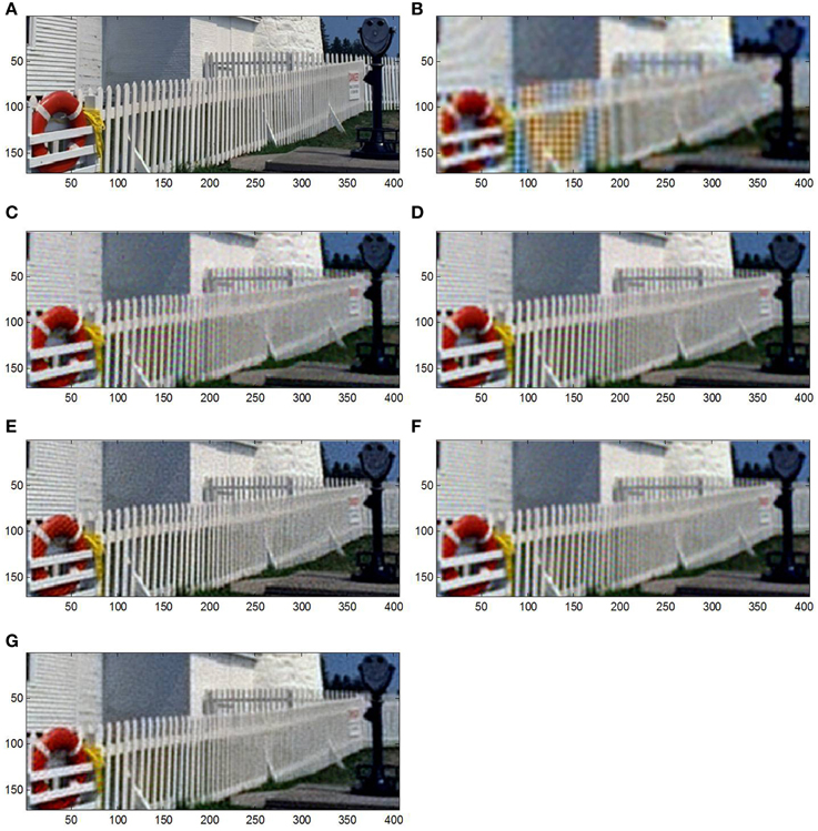
Figure 5. Simulated data results for (A) original HR image, (B) demosaic/interpolation, (C) MDSP SR, (D) RLS with independent color channel regularization, (E) color AWF SR, (F) independent color channel FIF SR, and (G) full FIF SR.

Table 1 contains quantitative results with the top two performers shown in bold type. The methods that operate on each color channel independently tend to provide better results than simple demosaic/interpolation because these approaches use multiple frames of information in the SR output. MDSP has generally similar performance to the independent channel methods. Color AWF has the best performance with full FIF SR slightly less in each metric. However, FIF SR provides more capability in handling complex global motion and local moving objects, as seen in subsequent experiments. This experiment also highlights the benefit of including cross-channel information in FIF SR. The full FIF approach provides nearly 20% (MSE) improvement over the independent channel FIF and performs much better by any metric.

TABLE 1

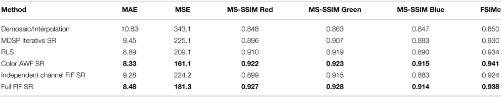
Table 1. Performance results for simulation experiment #1.

Global Translational Motion with Local Motion

The second simulation assesses performance in the presence of local motion. Since MDSP does not adapt for locally moving objects, it is not included. Here we compare performance to the robust RLS method and the version of color AWF SR modified to accommodate local motion.

We use the full-color (24-bit) Kodak barn image for this simulation. To create a locally moving object, we inserted a color chirp object into P = 10 HR images with the object moving at a constant rate across the image set. We then degrade the image as described in the previous simulation. This results in a set of LR Bayer CFA images with a moving object. The first and last HR input images and a simulated CFA frame are shown in Figure 6. The moving object is more challenging than expected in real imaging situations, but is used to stress the performance assessment.

FIGURE 6

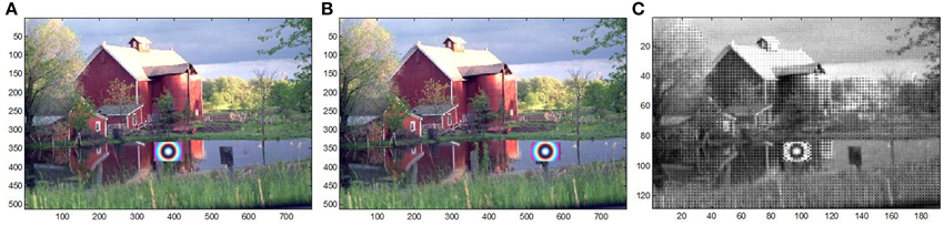
Figure 6. Simulated CFA images for local moving target experiment, (A) first frame and (B) last frame of synthetically generated HR image, and (C) simulated CFA image frame.

Cropped results are shown in Figure 7. We include the baseline color AWF output to highlight the effects when local motion is not accounted for. The modified color AWF output does reconstruct the moving object. However, the object and surrounding regions are not as sharp as the rest of the image since the method uses single frame SR in local motion regions. The FIF and robust RLS appear to provide the best visual results. However, robust RLS shows more artifacts in local motion regions since it also uses single frame data in any region of detected local motion.

FIGURE 7

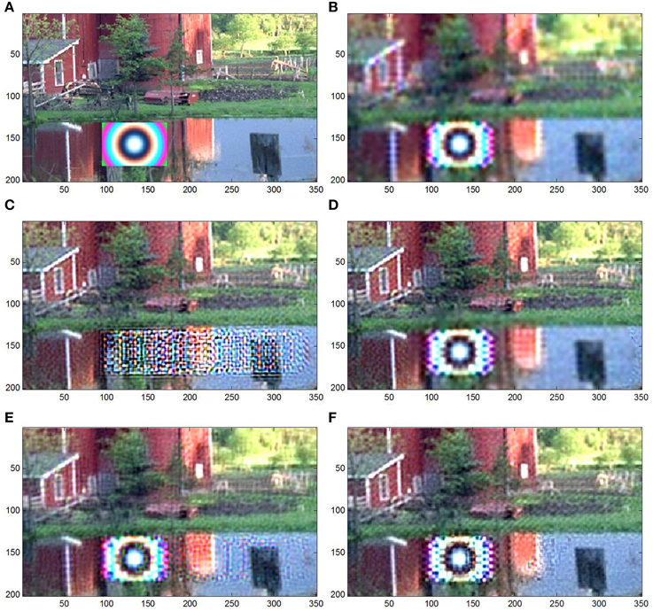
Figure 7. Simulated data results for global translational motion with local motion (A) original HR image, (B) demosaic/interpolation, (C) color AWF SR, (D) color AWF with local motion, (E) robust RLS, (F) FIF SR.

Table 2 shows quantitative results. Color AWF is excluded in the table since it was unable to reconstruct the local motion object. FIF and the modified color AWF provide the best reconstruction. The AWF method is able to maintain performance because local motion occurs in a relatively smooth region of the scene and global motion is limited to translation.

TABLE 2

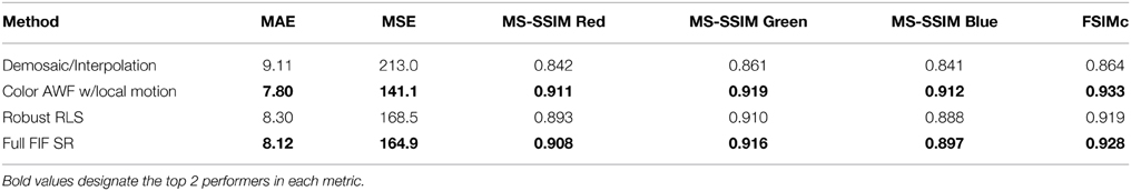
Table 2. Performance results for simulation experiment #2.

Global Affine Motion with Local Motion

For this experiment, global affine (translation and rotation) inter-frame motion is added to the previous experiment. The maximum rotation is 2.5°. Other than the inclusion of rotational motion, the simulation is the same as the prior experiment.

Figure 8 shows cropped results. Because demosaic/interpolation uses only the single reference frame, its performance is the same as the prior experiment. Artifacts are readily apparent in the modified color AWF SR output since it operates under a global translational motion assumption. In this experiment, we tested single frame color AWF SR, which performs better than multi-frame color AWF SR. Robust RLS and FIF results appear very similar to the prior experiment, demonstrating their capability to handle affine motion.

FIGURE 8

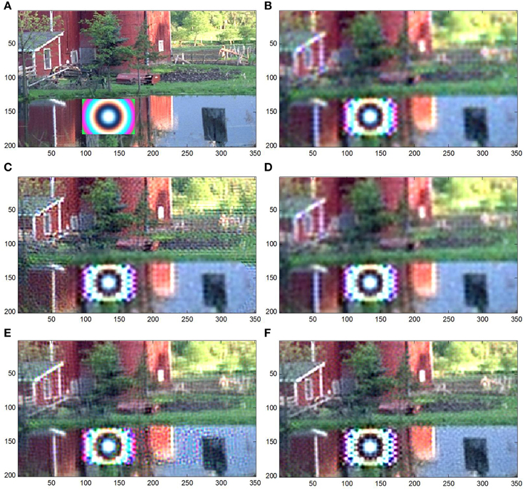
Figure 8. Simulated data results of affine motion with local motion for (A) original HR image, (B) demosaic/interpolation, (C) color AWF with local motion, (D) single frame color AWF SR, (E) robust RLS, (F) FIF SR.

Quantitative results are shown in Table 3. FIF SR provides the best results by any metric. Robust RLS performs slightly worse. For this simulation, the robust RLS method used 15 iterations for each channel. The total run time was about 14 min or approximately 19 s per iteration per channel. Total run time for the FIF method was about 11 s. While the implementations used un-optimized processing code, it is indicative of the relative ease in implementing these methods in real time. Additionally, since robust RLS is an iterative operation, it may be less amenable to parallel implementation to support real-time processing. Processing used MATLAB on a Windows 64-bit operating system with an Intel core i5 CPU with a 2.50 GHz clock speed and 8 GB of RAM.

TABLE 3

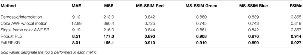
Table 3. Performance results for simulation experiment #3.

Real Data Experiments

Two real datasets were processed and examined. The first dataset collected Bayer CFA images using an Imaging Source DFK21BU04 CCD color camera that uses a 1/4” Sony ICX098BQ charge-coupled device (CCD) with a 640 × 480 sensor and 5.6 μm square detector elements. The camera does not have an anti-aliasing filter, making it appropriate for collecting test data. This camera collects images with a dynamic range of 8 bits. A variable lens set to f / 4 was used. A set of P = 10 frames was selected from a video sequence. The color channels are undersampled by 8.6×, 10.2×, and 12.4× for the red, green, and blue channels, respectively.

The second dataset is from an airborne MWIR panchromatic camera with f / 2.3 optics and 19.5 μm detector pitch. The camera's bandwidth is 3–5 μm, resulting in about 4.2× undersampling. This is the same MWIR dataset used in [10] and those results can be qualitatively compared to the results presented here.

Bayer CFA Camera

The Bayer color camera dataset contains affine inter-frame motion primarily consisting of rotation and a pencil is moved across a circular chirp panel. This creates a very challenging image set for two primary reasons. First, the chirp panel contains spatial frequency patterns and structures not typically seen in natural images. Also, the pencil has saturated color patterns and its shape comes to a sharp point. The object's movement across the chirp pattern highlights challenges in reconstructing the image in regions where the object moves across the set. Figure 9 shows the first and last frame of the set. The object moves from the bottom to the top of the scene and the rotational motion is apparent.

FIGURE 9

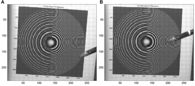
Figure 9. Images from Imaging Source color camera for global affine motion with local motion for (A) first and (B) last frame of the image set.

The following SR methods were applied for this assessment: demosaic/interpolation, color AWF SR with local motion, robust RLS, and FIF SR. Cropped ROI outputs are shown in Figure 10. Results are qualitatively comparable to the assessment described in the simulation experiment of Section Global affine motion with local motion. Demosaic/interpolation contains high levels of aliasing dominated by color fringing. Robust RLS does not effectively reduce this color fringing because of its independent channel operation. For primarily the same reason, the small color features in the moving pencil are not fully reconstructed.

FIGURE 10

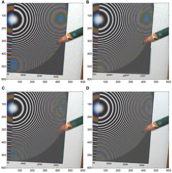
Figure 10. Imaging Source images for affine motion with local motion dataset, (A) demosaic/interpolation, (B) color AWF with local motion, (C) robust RLS, and (D) FIF SR.

The modified color AWF SR method reduces the color fringing in most of the scene and the moving object is reconstructed fairly well. However, in regions where the pencil motion is present in any frame, single frame AWF SR is applied and color fringing is quite apparent. Artifacts are also apparent at the edge of the panel due to rotational inter-frame motion.

FIF provides probably the best visual image quality. Color fringing is greatly reduced and FIF provides the best performance in the local motion region. Numbers along the bottom edge of the chirp pattern are clearest compared to the other methods. The most noticeable issue with FIF is the tip of the pencil not being fully reconstructed. This is caused because of an inherent trade in parameter selection between reducing the color fringing in the chirp pattern and completely reconstructing the pencil tip. Because real-world image set would not typically contain periodic spatial frequency structures, the trade for other datasets may likely involve increasing color fringing in order to fully reconstruct a small target.

Panchromatic MWIR Camera

For this experiment, the FIF method was modified to handle single channel data to compare FIF with the robust RLS since robust RLS was developed for panchromatic data. Bicubic interpolation is also included in the experiment. The SR improvement level was set to L = 4 and P = 10 frames were used. Figure 11 shows a cropped region from an input frame and SR results. These images capture a local moving object at the top of the image and sets of 4-bar resolution targets. Input data shows aliasing artifacts in the all resolution targets.

FIGURE 11

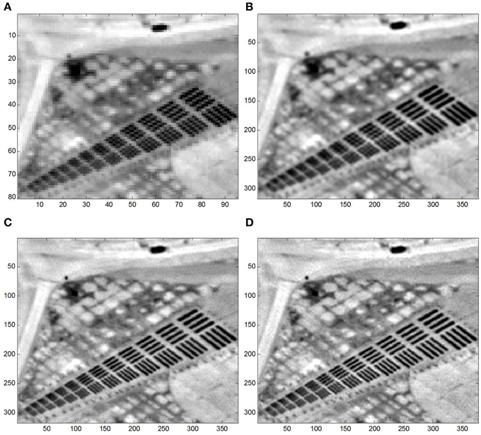
Figure 11. Section of real MWIR panchromatic data results for (A) input LR image, (B) bicubic interpolation, (C) robust RLS, (D) FIF SR.

Bicubic interpolation provides some improvement, resolving the first 2–3 sets of bars. Robust RLS and FIF perform demonstrate very good visual performance. They perform comparably to each other, resolving the bar patterns to about the 7th set of bars. Processing times were measured using un-optimized code and previously detailed processor specifications. For full LR image data (10 frames of 128 × 256 pixels per frame), the FIF method ran in approximately 4 s while the robust RLS method took about 200 s. For this experiment, RLS performed for 15 iterations, resulting in about 13 s per iteration.

Figure 12 shows the results for a second dataset. No local moving objects were in the data and the results are cropped to capture the bar pattern. These data highlight the aliasing effects with a different sample phasing than the prior results, as seen in the observed LR data for the vertical bar patterns. The SR results are the same as the prior dataset with robust RLS and FIF performing comparably. The horizontal bars are still resolved to the 6th or 7th set, but because of the sample phasing, the vertical bars are now resolved to about the 9th set.

FIGURE 12

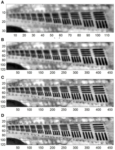
Figure 12. Section of second real MWIR panchromatic data results for (A) input LR image, (B) bicubic interpolation, (C) robust RLS, (D) FIF SR.

Conclusion

The FIF SR method is a straightforward and relatively fast approach that can handle SR processing in complex imaging conditions. We present the derivation of FIF utilizing temporal and cross-channel information in a unique weighted sum. Details of the weight components are provided showing how each component contributes to the proposed method.

The experimental results show the FIF method maintains performance with datasets that include affine global motion and local moving objects. While experiments focused on Bayer CFA cameras, airborne panchromatic camera data was also investigated. The FIF SR method performs comparably against other state-of-the-art SR methods in simpler constrained conditions and outperforms these methods in challenging realistic conditions. Because of its straightforward, non-iterative construction, the FIF method more readily lends itself to real-time implementation over more complex variational SR methods.

Conflict of Interest Statement

The authors declare that the research was conducted in the absence of any commercial or financial relationships that could be construed as a potential conflict of interest.

References

1. Hirakawa K, Wolfe PJ. Spatio-spectral color filter array design for optimal image recover. IEEE Trans Image Process. (2008) 17:1876–90. doi: 10.1109/TIP.2008.2002164

PubMed Abstract | Full Text | CrossRef Full Text | Google Scholar

2. Bayer BE. Color Imaging Array. U.S. Patent 3,971,065. Rochester, NY: Eastman Kodak Co. (1976).

Google Scholar

3. Ramanath R, Snyder, W, Bilbro G, Sander W. Demosaicking methods for the Bayer color arrays. J Electron Imaging (2002) 11:306–15. doi: 10.1117/1.1484495

PubMed Abstract | Full Text | CrossRef Full Text | Google Scholar

4. Gunturk BK, Glotzbach J, Altunbasak Y, Schafer RW, Mersereau RM. Demosaicking: color filter array interpolation. IEEE Signal Proc Mag. (2005) 22:44–54. doi: 10.1109/MSP.2005.1407714

CrossRef Full Text | Google Scholar

5. Li X, Gunturk B, Zhang L. Image demosaicing: a systematic survey. In: Proc. SPIE 6822. (2008) p. 68221J.

Google Scholar

6. Fiete RD. Image quality and λFN/p for remote sensing systems. Opt Eng. (1999) 38:1229–40. doi: 10.1117/1.602169

CrossRef Full Text | Google Scholar

7. Park SC, Park MK, Kang MG. Super-resolution image reconstruction: a technical overview. IEEE Signal Proc Mag. (2003) 3:21–36. doi: 10.1109/MSP.2003.1203207

PubMed Abstract | Full Text | CrossRef Full Text

8. Milanfar P. Super-Resolution Imaging. Boca Raton, FL: CRC (2010).

9. Hardie RC. A fast super-resolution algorithm using an adaptive Wiener filter. IEEE Trans Image Process. (2007) 16:2953–64. doi: 10.1109/TIP.2007.909416

PubMed Abstract | Full Text | CrossRef Full Text | Google Scholar

10. Hardie RC, Barnard KJ, Ordonez R. Fast super-resolution with affine motion using an adaptive wiener filter and its application to airborne imaging. Opt Express (2011) 19:26208–31. doi: 10.1364/OE.19.026208

PubMed Abstract | Full Text | CrossRef Full Text | Google Scholar

11. Karch BK, Hardie RC. Adaptive wiener filter super-resolution of color filter array images. Opt Express (2013) 21:18820–41. doi: 10.1364/OE.21.018820

PubMed Abstract | Full Text | CrossRef Full Text | Google Scholar

12. Tanaka M, Okutomi M. Towards robust reconstruction-based superresolution. In: Milanfar P, editor. Super-Resolution Imaging. Boca Raton, FL: CRC Press (2010). p. 219–46.

Google Scholar

13. Kim M, Ku B, Chung D, Shin H, Han D, Ko H. Robust video super resolution algorithm using measurement validation method and scene change detection. EURASIP J Adv Signal Process. (2011) 2011:1–12. doi: 10.1186/1687-6180-2011-103

CrossRef Full Text | Google Scholar

14. Zhang Z, Wang R. Robust image superresolution method to handle localized motion outliers. Opt Eng. (2009) 48:077005. doi: 10.1117/1.3159871

CrossRef Full Text | Google Scholar

15. Dijk J, van Eekeren AWM, Schutte K, de Lange, D-JJ, van Vliet LJ. Superresolution reconstruction for moving point target detection. Opt Eng. (2008) 47:096401. doi: 10.1117/1.2977790

CrossRef Full Text | Google Scholar

16. El-Yamany NA, Papamichalis PE. Robust color image superresolution: an adaptive m-estimation framework. EURASIP J Adv Signal Process. (2008) 2008:1–12. doi: 10.1155/2008/763254

CrossRef Full Text | Google Scholar

17. Park MK, Kang MG, Katsaggelos AK. Regularized high-resolution image reconstruction considering inaccurate motion information. Opt Eng. (2007) 46:117004. doi: 10.1117/1.2802611

PubMed Abstract | Full Text | CrossRef Full Text | Google Scholar

18. Ivanovski ZA, Panovski L, Karam LJ. Robust super-resolution based on pixel-level selectivity. In: Proc. SPIE, Vol. 607707. San Jose, CA (2006).

19. Farsiu S, Robinson D, Elad M, Milanfar P. Fast and robust multi-frame super-resolution. IEEE Trans Image Process. (2004) 13:1327–44. doi: 10.1109/TIP.2004.834669

PubMed Abstract | Full Text | CrossRef Full Text | Google Scholar

20. Farsiu S, Robinson D, Elad M, Milanfar P. Advances and challenges in super-resolution. Int J Imaging Syst Tech. (2004) 14:47–57. doi: 10.1002/ima.20007

CrossRef Full Text | Google Scholar

21. Hardie RC, Barnard KJ. Fast super-resolution using an adaptive wiener filter with robustness to local motion. Opt Expr. (2012) 20:21053–73. doi: 10.1364/OE.20.021053

PubMed Abstract | Full Text | CrossRef Full Text | Google Scholar

22. Shimizu M, Yano T, Okutomi M. Super-resolution under image deformation. In: International Conference on Pattern Recognition, Vol. 3. Cambridge, UK (2004) p. 586–9.

23. Gotoh T, Okutomi, M. Direct super-resolution and registration using raw CFA images. In: Proceedings of the 2004 IEEE Computer Society Conference on Computer Vision and Pattern Recognition, Vol. 2. Washington, DC (2004) p. 600–7.

24. Sasahara R, Hasegawa H, Yamada I, Sakaniwa K. A color super-resolution with multiple nonsmooth constraints by hybrid steepest descent method. In: IEEE International Conference on Image Processing, Vol. 1. Genoa (2005) p. 857–60.

25. Farsiu S, Elad M, Milanfar P. Multiframe demosaicing and super-resolution of color images. IEEE Trans Image Proc. (2006) 15:141–59. doi: 10.1109/TIP.2005.860336

PubMed Abstract | Full Text | CrossRef Full Text | Google Scholar

26. Gevrekci M, Gunturk BK, Altunbasak Y. POCS-based restoration of Bayer-sampled image sequences. In: IEEE International Conference on Acoustics, Speech and Signal Processing, Vol. 1. Honolulu, HI (2007) p. 753–56.

27. Li YR, Dai DQ. Color superresolution reconstruction and demosaicing using elastic net and tight frame. IEEE Circ. (2008) 55:3500–12. doi: 10.1109/TCSI.2008.925369

CrossRef Full Text | Google Scholar

28. Trimeche M. Color demosaicing using multi-frame super-resolution. Eur Signal Process Conf. (2008).

Google Scholar

29. Sorrentino DA, Antoniou A. Improved hybrid demosaicing and color super-resolution implementation using quasi-Newton algorithms. In: Canadian Conference on Electrical and Computer Engineering. St. John's, NL (2009) p.815–8.

30. Oppenheim A, Schafer R. Discrete-Time Signal Processing. Englewood Cliffs, NJ: Prentice Hall (1989).

Google Scholar

31. Malvar HS, He LW. Cutler R. High-quality linear interpolation for demosaicing of Bayer-patterned color images. In: International Conference of Acoustic, Speech and Signal Processing, Vol. 3. Upper Saddle River, NJ (2004) p. 485–8.

Google Scholar

32. Lucas BD, Kanade T. An iterative image registration technique with an application to stereo vision. In: International Joint Conference on Artificial Intelligence, Vol. 81. Montreal, QC (1981) p. 121–30.

33. Bergen JR, Anandan P, Hanna KJ, Hingorani R. Hierarchical model-based motion estimation. Comput. Vis. ECCV'92 (1992) 11:237–52.

Google Scholar

34. Glassner AS. Graphics Gems. Vancouver, BC: Academic Press (1990).

Google Scholar

35. Goossens B, Luong Q, Pizurica A, Philips W. An improved non-local denoising algorithm. 2008 Int'l Workshop Local Non Local Approx Image Process. (2008) 588:143–56.

Google Scholar

36. Shao M, Barner KE, Hardie RC. Partition-based interpolation for image demosaicking and super-resolution reconstruction. Opt Eng. (2004) 44:107003–1. doi: 10.1117/1.2087428

CrossRef Full Text

37. Gevrekci M, Gunturk BK, Altunbasak Y. Restoration of Bayer-sampled image sequences. Comput J. (2009) 52:1–14. doi: 10.1093/comjnl/bxm041

CrossRef Full Text | Google Scholar

38. Gunturk BK, Altunbasak Y, Mersereau RM. Color plane interpolation using alternating projections. IEEE T. Image Process. (2002) 11:997–1013. doi: 10.1109/TIP.2002.801121

PubMed Abstract | Full Text | CrossRef Full Text | Google Scholar

39. Cok DR. Signal Processing Method and Apparatus for Producing Interpolated Chrominance Values in a Sampled Color Image Signal. Oxford:, UK Eastman Kodak Co., U.S. Patent No. 4,642,678 (1987).

Google Scholar

40. Adams JE Jr. Design of practical color filter array interpolation algorithms for digital cameras. Electronic Imaging'97 (1997) 117–25.

Google Scholar

41. Kimmel R. Demosaicing: image reconstruction from color CCD samples. IEEE T. Image Process. (1999) 8:1221–8. doi: 10.1109/83.784434

PubMed Abstract | Full Text | CrossRef Full Text | Google Scholar

42. Pei SC, Tam IK. Effective color interpolation in CCD color filter arrays using signal correlation” IEEE Circ Syst Vid. (2003) 13:503–13. doi: 10.1109/TCSVT.2003.813422

CrossRef Full Text | Google Scholar

43. Smith AR. Color gamut transform pairs. ACM Siggraph Comput Graph. (1978) 12:12–9. doi: 10.1145/965139.807361

CrossRef Full Text | Google Scholar

44. Zhang F, Wu X, Yang X, Zhang W, Zhang D. Robust color demosaicking with adaptation to varying spectral correlations. IEEE T. Image Process. (2009)18:2706–17. doi: 10.1109/TIP.2009.2029987

PubMed Abstract | Full Text | CrossRef Full Text | Google Scholar

45. Gonzalez R, Woods R. Digital Image Processing. Prentice Hall. (2008).

Google Scholar

46. Jain AK. Fundamentals of Digital Image Processing. Englewood Cliffs, NJ: Prentice Hall. (1989).

47. Hardie RC, Barnard KJ, Bognar JG, Armstrong EE, Watson EA. High-resolution image reconstruction from a sequence of rotated and translated frames and its application to an infrared imaging system. Opt Eng. (1998) 37:247–60.

Google Scholar

48. Wang Z, Simoncelli EP, Bovik AC. Multiscale structural similarity for image quality assessment. In: Conference Record of the Thirty-Seventh Asilomar Conference on Signals, Systems and Computers, Vol. 2. Pacific Grove, CA (2003) p. 1398–402.

49. Zhang L, Zhang D, Mou X. FSIM: a feature similarity index for image quality assessment. IEEE T. Image Process. (2011) 20:2378–86.

PubMed Abstract | Full Text | Google Scholar