Transport efficiency and dynamics of hydraulic fracture networks

Introduction

Fluid flow in the Earth's crust is evidenced by a variety of geological phenomena, including veins and hydraulic breccias. Veins are dilatant structures, typically fractures, filled with minerals that precipitated from fluid (see review of [1], and references therein). Hydraulic breccias are fragmented rocks where the fragmentation is mainly caused by chaotic fracturing due to fluid overpressure [2–5], as opposed to tectonic breccias where the diminution is due to tectonic stresses, typically along faults [6–8].

Both veins and breccias usually show evidence for repeated fracturing. Veins commonly exhibit microstructures that are indicative of the “crack-seal mechanism” [9], where a crack repeatedly opens and is subsequently sealed again by mineral growth (Figure 1). This crack-sealing, which can be repeated thousands of times in a single vein, indicates that fluid flow is not continuous, but intermittent: fluid pressure builds up to exceed the tensional strength of the rock and cause failure, after which flow can occur until the fracture permeability is sealed off again [9–13]. Hydraulic breccias also typically show indications of repeated fracturing in the form of clasts in clasts and brecciated cement [4, 14].

FIGURE 1

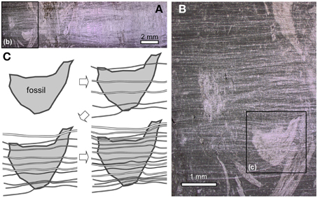
Figure 1. Microphotograph and sketch of a crack seal vein from fossiliferous Cretaceous limestone in the Jabal Akhdar Dome, Oman [20]. (A) Overview of one half of the vein, composed of hundreds of individual crack-seal veinlets. (B) Distributed crack-seal veinlets, each tens of μm in width are visible in a close up. (C) Schematic development stages of the vertcially stretched fossil fragment in (B). The actual order of fracture events cannot be determined from the thin section image. Plane-polarized light.

Although evidence for intermittent fluid flow is abundant, relatively little is known on the duration of and time spans between fracturing events. An indirect indication can be achieved by considering fluid flow velocities and total fluxes. Theoretical considerations of fracture propagation velocity, and hence velocity of contained fluid, range from m/yr to m/s [15, 16]. The large range is mostly due to uncertainty in the fracture toughness of rocks. Field observations suggest that flow velocities can reach the upper end of the range. For example, [17] and [18] estimated flow velocities of 0.01–0.1 m/s from the size of grains that were carried up by the fluid. Using similar arguments, [24] derived flow velocities in excess of 5 m/s in a fluidized breccia with m-sized clasts from the Cloncurry District, Australia.

Weisheit et al. [4] describe a hydraulic breccia, the Hidden Valley Breccia, Australia, that is 10 km² in outcrop and contains clasts that range from < 0.1 mm to >100 m in size. It formed over a period of more than 150 million years, as basement gneisses were exhumed in this area by over 12 km [19]. The estimated amount of fluid to have produced this breccia is about 20 km³. Assuming a porosity of 10% and a flow rate of 1 m/s, at the upper end of the aforementioned range, the estimated duration of flow (Δt) would only be about 2100 s, or a mere few hours. This is a minute fraction of the >100 million years it took to form the breccia. Even if the flow rate was 1 m/yr, the total duration would only be about 2100 years. Fluid flow must therefore have been highly intermittent with only very occasionally short bursts of flow, and extremely long periods of pressure buildup. This mechanism can result in dense networks of veins composed of many crack-seal events that formed over long periods of time [e.g., 20].

Intermittent flow is predicted to occur when the matrix permeability of a rock is insufficient to accommodate fluid flow [21, 22]. This leads to an increase in fluid pressure and opening of hydrofractures. When exceeding a critical length, these can become mobile by propagation on one end and closure at the other. Such “mobile hydrofractures” thus propagate together with their contained fluid and can reach velocities in the order of m/s [16, 22, 23]. Possible fluid sources which may generate the necessary fluid pressure for hydraulic brecciation and hydraulic fracturing are fluid released by igneous intrusions [24], fluid release due to decompression [25, 26] or mineral dehydration reactions [27]. Dehydration of the mineral biotite appears to be the main fluid source in case of Hidden Valley [4].

In contrast, classically large-scale fluid flow is assumed to take place by slow, convective fluid percolation, typically driven by topography or thermal instabilities, for example due to igneous intrusions [28, 29]. Such convective flow requires a fluid pressure that is close to hydrostatic, which is incompatible with the high, supra-lithostatic fluid pressures required to fracture rocks to produce veins and breccias [1].

A number of numerical models for hydrofracture formation exist already [30, 31] while new models are continuously developed [e.g., 32–36]. The current interest in these models is mainly triggered by the enormous economic importance of artificial hydraulic (aka “fracking”) as a means of oil and gas extraction. However, these models are focused on the micro- to meso-scale, where single cracks and fractures can be numerically resolved. Existing numerical models for crustal scale flow, on the other hand, do not consider the interplay between fluid flow and hydraulic fracturing, but assume that the intrinsic matrix permeability of rocks is the only relevant parameter [e.g., 37–39]. Miller and Nur [21] developed a crustal scale cellular automaton model which was able to capture the general dynamics of large scale hydraulic fracture networks, but wasn't based on realistic concepts for fluid propagation and closing of fractures.

To our knowledge, the numerical model developed and applied in this study is the first discrete crustal scale 2D model which integrates fluid flow dynamics and hydrofracture formation. This setup permits modeling of dynamic hydraulic fracture networks and the derivation of the key control factors. The setup is intentionally simple compared to the “real” crust, since we are interested in the general characteristics of the fracture patterns and the efficiency of the transport mechanism.

Below we first show that the transport mechanism of crustal fluid must include hydraulic fracturing in order to explain the hydraulic rocks at Mount Painter. In a second step we investigate the hydraulic fracture patterns which develop in a simplified crust in a 2D model. We exclude the consideration of finer geological intricacies in the model, e.g., geological layering. Of more importance in this context are the influence of a crustal scale pressure gradient and the rate of closure of hydraulic fractures.

Fluid Flow and Hydraulic Fracturing in the Earth's Crust

The basic law governing laminar fluid flow q over a distance L through porous media is Darcy's law:

$\begin{array}{cc}q=K\frac{\Delta \left(P_f-{\rho }_{H_{2}O}gz\right)}{L},& \left(1\right)\end{array}$

where ρ_H2O is the density of water, P_f the fluid pressure, g earth's acceleration, K the hydraulic conductivity, L the distance and z the height difference between start point and end point of the fluid flow. In case of vertical fluid flow, and with reference to the surface, L = z and P_{f, surface} = 0.

It is commonly assumed that fluid overpressure causes tensile fracturing [e.g., 33, 40, 41, 43]. Therefore, fluid pressure is non-destructive as long as one of the following relation holds, which are commonly applied fracture conditions [compare for instance [33, 44, 47]:

$\begin{array}{cc}{P}_f<{\sigma }_3+P_{cr}& \left(2\right)\end{array}$

or

$\begin{array}{cc}{\sigma }_1-{\sigma }_3\ge 4P_{cr}& \left(3\right)\end{array}$

where σ₁ and σ₃ are the maximum and minimum principal normal stress in the solid and P_cr is the tensile strength of the material. Here, tensile stress is negative.

The state of stress in the crust is probably among the most controversial issues in geology/geophysics. While it is generally safe to assume hydrostatic conditions for the fluid pressure, the conditions for solid stress in the crust are a topic of continuous debate. Elastic theory links uniaxial vertical loading stress to the horizontal stress via a function of the Poisson ratio μ, which is typically about 0.2–0.3 for geological materials. However, new data [48] suggests that solid stress in the crust is approximately isotropic if external tectonic stress is absent and below c. 1000 m depth., i.e., σ₃ ≈ σ₁. The reason is that the loading stress is mainly compensated by brittle plastic deformation at this depth.

We apply this criterion in the numerical model, which means that we effectively adapt the so-called lithostatic stress model [e.g., 49], which assumes isotropic solid stress conditions. This choice has been partly made because one of the specific aims of this study was to use a simplified model, and to focus on the driving forces. The driving force for hydraulic fracturing is mainly the fluid pressure, independent of a specific crustal stress model, due to the nature of the fluid pressure gradient.

This means that the modeled solid stress field is probably not exactly correct very close to the surface. However, the range of possible horizontal stress values that has been reported is large and includes the isotropic stress case (σ_v/σ_h = 1) till approximately 250 m depth [48]. Since we are concerned with the fluid flow at a larger depth rather than in surface vicinity, this was considered an acceptable compromise. This compromise deems even more acceptable as we have to assume a permanent open fracture network close to the surface, whose non-dynamic behavior is not within the scope of interest for this study.

Under these conditions the criterion for failure is simply:

$\begin{array}{cc}-P_{eff}>P_{cr},& \left(4\right)\end{array}$

where P_eff = σ₃ − P_f is the effective pressure. The overpressure P_o is defined as P_o = −P_eff, if P_eff < 0. Obviously, hydraulic fracturing occurs if P_o > P_cr.

Figure 2A shows the idealized increase of fluid and solid stress with depth. Due to different gradients of fluid pressure and solid pressure (P_s) the difference between P_eff and P_s increases with depth. Therefore, at large depth a required fluid pressure in order to initialize hydraulic fracturing is larger than at a shallower depth. This has the additional effect that the fluid pressure gradient in the vicinity of a fluid source is often higher at large depth than it is at shallower crustal levels, resulting in larger flow velocities on fractures at depth (Equation 1). Another effect of the different fluid and solid pressure gradients is the potential formation of mobile hydraulic fractures (Figure 2B, [1]).

FIGURE 2

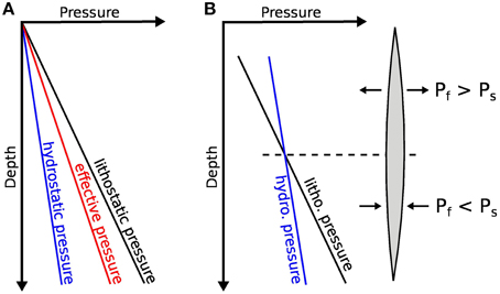
Figure 2. (A) Idealized pressure gradients in the Earth's crust. Due to its higher density, the lithostatic (solid) pressure increases with depth faster than the hydrostatic (fluid) pressure. The effective pressure (P_eff = P_s − P_f) is in-between. (B) Formation of mobile hydrofractures [after 1]. The different pressure gradients of fluid and solid lead to fluid overpressure in the upper part of a fracture and to fluid underpressure at the lower part of the fracture. The fracture moves upward. Please note that the average fluid pressure in a hydraulic fracture is identical to the pressure in the solid.

Equation (1) in combination with the criterion for hydraulic fracturing (Equations 2–4) permits the calculation of the necessary minimum conductivity that crustal rocks must have in order to conduct fluid flow with a given flow rate. A potential fluid source in the Earth's crust are metamorphic dehydration reactions, which are caused by changing pressure and temperature conditions.

For simplicity we consider the mineral reaction biotite → feldspar + Fe/Mg-oxide + water as the single fluid source, which has been suggested for the Mount Painter breccias [4]. We further assume that the reaction occurs at a depth of 16 km depth [e.g., 4, 50]. With a tensile strength of 1 MPa [44] the fluid pressure is very close to the lithostatic pressure if hydraulic fracturing is initiated. If we assume a volumetric flux of 1 m/s, which has been suggested for Mount Painter, a necessary minimum conductivity of approximately 6 × 10⁻⁵ m/s for the conducting material follows from Equation (1). The conductivity of non-fractured crustal material is approximately in the range of 10⁻⁹–10⁻¹² ms/s [43], several orders of magnitude too small to allow the necessary fluid flow from the source zone to the surface.

It must be concluded that fluid transport on the scale as observed at Mount Painter can occur only along fractures. These fractures may be either stationary or dynamic and mobile, depending on the evolution of the fluid stress field and the rate of fracture closure/healing once the fluid pressure decreases. If fractures heal slowly enough, fractures remain open between intermittent fluid pulses, and the fracture network is therefore stationary. The most dominant contributions to the closure of fractures are healing (plastic deformation; [49], see also Figure 4) and sealing (e.g., due to mineral precipitation or cataclasis; [40]).

Numerical Model

The computer model consists of a 2D section of crustal dimensions through a material with constant porosity and conductivity of the undamaged rock matrix, which represents a simplified Earth's crust. Fluid flow through porous rocks and through fractures can be modeled as Darcian flow, using Equation (1). We solve the Darcy equation with a Monte Carlo approach applied to an explicit finite difference solution on a regular square grid, which allows the computation of fluid flow in highly anisotropic and heterogeneous media. The nodes in this grid represent fractured or undamaged material with two different predefined hydraulic conductivities (Table 1). Fractures can be either horizontally or vertically oriented, therefore the fracture conductivity is anisotropic.

TABLE 1

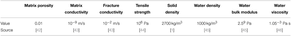
Table 1. Material parameters used in the simulations.

Fracture nucleation and fracture propagation are distinctly different steps in the simulations. Nucleation takes place once fluid pressure at a node is sufficiently high to cause fracturing in either the horizontal or vertical direction, according to the fracture criterion outlined in Equations (2–4). In order to model the inherent disorder of the material, Gaussian noise is applied to the tensile strength of the nodes and to the conductivity of fractures. The solid stress is considered to be isotropic (see cp the discussion in Section Fluid Flow and Hydraulic Fracturing in the Earth's Crust), meaning that fracture nuclei increase conductivity in both directions, horizontal and vertical.

In the numerical model a layer of constant overpressure at the lower model boundary serves as the fluid source. This allows us an assessment of the efficiency of the fluid transport in the system as the effective conductivity of the system once the system reaches a state of dynamic equilibrium. We coined the term “effective conductivity” for this study, which describes the averaged conductivity from the source at the lower boundary to the sink at the surface. Other fluid sources, for instance a constant production of fluid mass instead of constant pressure, wouldn't allow a similarly simple description of the system.

The overpressure at the lower system boundary is freely selectable in each simulation. The rate of fluid production is therefore a direct function of the efficiency of the fluid transport from the source to the surface. Geologically, this might represent a pressure controlled fluid-producing mineral reaction.

Nodes are assumed to be mechanically coupled, which is a typical assumption for the formation and propagation of hydraulic fractures [e.g., 40, 51]. Thus, fractures propagate if the fluid stress at an already fractured node is sufficiently high to fulfill the fracture condition at a neighboring node too:

$P_s^n-P_f<P_{cr}^n,$

where the superscript n refers to the neighbor node (Figure 3).

FIGURE 3

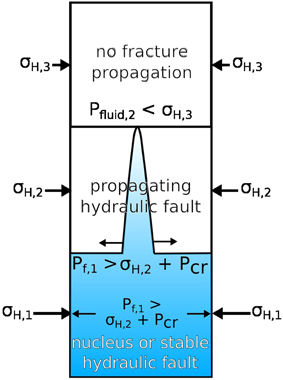
Figure 3. Fractures propagate if the fluid pressure at a neighboring, already fractured node is larger than the local fracture criterion. Here, a vertical fracture propagates from layer 1 to layer 2, where it is arrested. σ_H, horizontal solid stress; P_f, fluid pressure; P_cr, critical stress.

Time stepping is often a non-trivial issue in the modeling of geological processes, where long-term processes cause and interact with dynamic processes on far shorter time scales. The computer simulations use adaptive time steps with a fixed maximum Δt_max. Time steps Δt are determined by an estimate of the minimum time it takes to build up sufficient pressure at the existing fracture tips to cause further fracture propagation. If this time estimate is larger than Δt_max, Δt is set to Δt_max.

Closing and healing of fractures is a complex process, which involves elastic and viscous closure of the fracture and dissolution and precipitation of minerals within the fracture former fracture aperture. Here we assume that a fracture is closed by viscous flow of the solid matrix into irregularities of the fault surface once P_eff > 0 only, an assumption which is suitable for the given fundamental assumption of damage zones or tectonic breccias rather than discrete faults with clear cut parallel walls (cp Figure 4). Because the impact of the fracture closure rate on the dynamics of the fracture network is one of the major interests in this study, the solid viscosity is considered homogeneous throughout the entire system. The fracture aperture is a function of the former fluid overpressure in the fracture and is calculated by a solution adapted from Maugis [51].

FIGURE 4

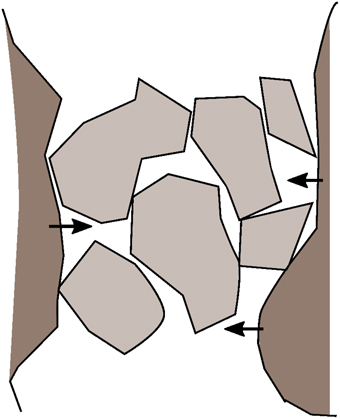
Figure 4. Model for the closure of a fractured area by viscous flow of the solid into the fractured rock. The fracture is assumed to be formed by fractured clasts rather than by clear cut fracture walls. These clasts act as barriers against a simple elastic closure of the fracture once fluid pressure within the fracture zone is smaller than the solid pressure. Therefore, the fracture closes by viscous flow of the surrounding rock into the cavities made up by the clasts.

Setup of Numerical Simulations and Results

General Setup

Material parameters are compiled in Table 1. The following parameters are identical in all conducted simulations: the system size is 8000 (horizontal) by 16,000 m (vertical), with a distance Δl between fluid source and fluid sink of 15,750 m. A resolution of 100 × 200 grid points is commonly used, but has been occasionally compared to results with a solution of 150 × 300 in order to test the resolution dependency of the model. Gaussian normal distribution on the tensile strength of nodes assumes a mean strength of 1 MPa and a standard deviation of 0.1 MPa. The basal source layer with constant fluid overpressure P_o = const and the fluid sink with P_f = 0 Pa are located at opposed system boundaries.

Modeling of individual fractures and fracture planes in a crustal scale model requires a resolution which is not achievable with today's computational equipment. The model therefore assumes that fractures form as fracture networks and affect the entire area defined by a gridpoint. Comparing the results from simulations with different resolutions did not show a change of the system behavior regarding fracture mobility and fluid transport efficiency.

In order to test the influence on the dynamics of the fracture network, P_o of the fluid source is varied between 0.5 and 2.0 MPa during the simulations and the solid viscosity ν between 10¹⁷ and 10²³ Pa s, which can be assumed to be close to the geologically realistic lower and upper limit [52, 53]. We assume here that fractured nodes have the same conductivity as a typical sedimentary breccia [54–56], since fracturing in the crust typically results in the formation of a damage zone rather than an isolated fracture plane [34, 57].

The choice of a crustal stress model is a rather difficult one since the topic is still under intense debate. The model assumes a isotropic lithostatic solid stress, which is probably a good approximation in case of a vertical crustal section, given that the depth is considerably larger than ~1 km and external tectonic forces are absent (compare discussion in Section Fluid Flow and Hydraulic Fracturing in the Earth's Crust). This assumption ignores natural variations in the horizontal stress field, which are frequently observed drill-holes, but are difficult to quantify in a model [58, 59].

Experiments in a System without Pressure Gradient (“Horizontal” Profile)

In order to test the influence of the pressure gradient on the dynamics of fracture formation and propagation, we compare the time evolution of hydraulic fractures through a vertical 2D section through the crust (Δz = 16.000 m) with a horizontal section (Δz = 0 m). Fluid stress is constant in the case of a horizontal section, i.e., dP_f/dL = 0.

Figure 5 displays the resulting hydraulic fracture pattern, the fluid mass change with time (Δm_f/t) and the fractured area in the horizontal system. The fluid source is located at the left system boundary with a constant overpressure P_o = 1.2 MPa while the sink is at the right of the system. Thus, the hydraulic head over the entire system length is ΔH = ΔP = 1.2 MPa, identical to simulations set in a vertical profile.

FIGURE 5

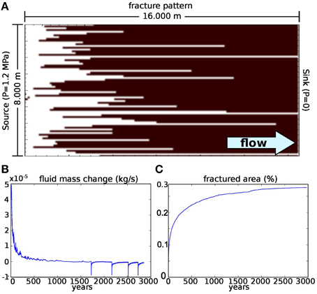
Figure 5. Final fracture pattern (A), fluid mass change with time (Δm_f/t) (B) and total fractured area in % (C) in an simulation where the hydraulic fracture propagation is calculated for a horizontal 2D section through the crust, i.e., in the absence of an initial pressure gradient. The situation is somewhat similar to flow to a well. Low viscosity conditions (ν = 10¹⁷ Pa s), i.e., fractures close quickly. (A) Fractured nodes are white. Fluid source is a constant layer with constant fluid pressure P_f = 1.2 MPa at the left boundary of the model, the sink is at the right boundary with constant P_f = 0 Pa, similar to experiments with vertical fracture propagation. Fractures propagate until the source is sufficiently connected to the sink, at which point flow becomes stable. The fracture network is stationary, even though the viscosity is low. The fluid mass in the system remains constant from this point on (B). Negative peaks are created by rapid drainage of the system fluid mass when a fracture reaches the other side and fluid pressure is rapidly released. From 3000 a onwards no further fracturing occurs. (C) Propagation of the fracture front is fast at the beginning, then slows down and converges against zero, which is indicated by a constant percentage of fractured material in the system.

The final fracture network that develops in these experiments is stationary. Close to the source a fracture front develops, which is replaced by individual fractures once the front reaches a certain distance from the sink (Figure 5). Fractures do not close once formed but maintain sufficient fluid overpressure to keep existing fractures open.

If fractures penetrate the sink, a large amount of fluid is quickly drained into a fluid burst, creating the large negative peaks in Figure 5B. Once a sufficient number of fractures reach the sink, an equilibrium between fluid production and fluid drainage is reached and the fluid mass remains approximately constant (Figure 5, constant conditions are reached from 3000 years onward). From this point on the fracture pattern is stationary. Due to the constant fluid overpressure in fractures, the fracture viscosity is irrelevant to the development of the fracture network and the fault patterns are identical whether ν = 10¹⁷ or 10²³ Pa s. Negative spikes in the fluid mass change between 1500 and 2700 years (Figure 5B) correlate with the permanent opening of single fractures, which cause sudden and very efficient drainage resulting in a short dewatering event. Once the fracture network is efficient enough to provide continuous pathways from the source to the sink, both the fracture distribution and the fluid mass in the system remain constant.

Unlike the vertical experiments described below, we were unable to establish a permanent pulsating regime in these experiments. If the fluid pressure at the source is to small, flow occurs within the rock matrix. If pressure is high, a stable fracture pattern develops, where the total number of fractures increases with the pressure at the source. Dynamic flow and fracture formation, however, seem to rely on the presence of a fluid pressure gradient, as in the numerical simulations discussed below.

Experiments with Fluid Pressure Gradient (Vertical Profile)

If basal fluid overpressure is sufficiently large (starting already at P_o ≈ 0.8 MPa, due to the noise on the tensile strength), hydraulic fractures form and drain the fluid produced at the basal fluid source toward the surface. In all experiments the fractured area increases until the fracture network is efficient enough to create equilibrium between fluid production at the basal fluid source and fluid drainage at the surface.

Two sets of simulations have been computed: one set with ν = 10¹⁷ and 10²³ Pa s (Figures 6–10). A detailed description follows in the sections below. The fluid overpressure of the fluid source was varied between 0.5 and 2.0 MPa. The characteristic values in Figures 6, 9—the fractured area and the balance between fluid production and fluid drainage Δm_f/t—reach near-stable plateaus with recurring patterns, indicating that the system is in a dynamic or stable equilibrium (discussed in Section Intermittency of Fluid Flow).

FIGURE 6

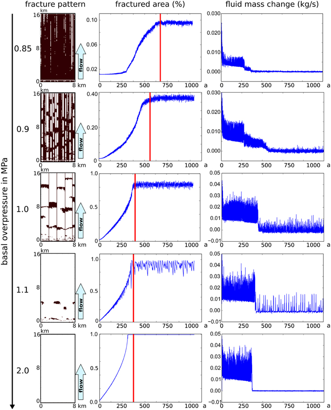
Figure 6. Final fracture pattern, fluid mass change (Δm_f/t) and total fractured area in % in experiments with vertical hydraulic fracture propagation at low viscosity ν = 10¹⁷ Pa s. Fractured nodes are white. Fluid source is a constant layer with constant fluid overpressure at the bottom boundary of the model. The sink is at the top boundary with constant fluid pressure P_f = 0 Pa, representing a free surface. With increasing overpressure, the total fractured area increases until the entire system is damaged. Fracture clusters are dynamic and are mobile in the vertical direction, moving upwards. The horizontal position is fixed and determined by the Gaussian noise. Stable fracture patterns occur at fixed basal overpressures of 0.5 and 2.0 MPa. Periodic changes of the fractured area and of the fluid mass, even after fluid production and fluid drainage are in equilibrium, illustrate the dynamic nature of the fracture pattern and the fluid flow. Red line: From the marked time step onward the system is considered to be in a stable state. Power spectral density in Figure 11 is calculated for the stable state.

FIGURE 7

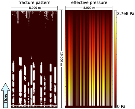
Figure 7. Fracture pattern and effective stress at an intermediate state of the development of the fracture network with ν = 10¹⁷ Pa s. Vertical experiment with fixed basal overpressure of 0.9 MPa (cp. Figure 6). An initial front of mobile fractures develops early on in the development, generating columns of increased fluid pressure. This leads to the formation of vertical hydraulic fractures nucleating at and propagation downward from the surface, where the difference between hydrostatic fluid pressure and lithostatic pressure is small (cp. Figure 2).

FIGURE 8

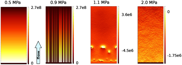
Figure 8. Effective stress fields after equilibrium between fluid production and drainage is reached in vertical experiments with viscosity ν = 10¹⁷ Pa s. Preferred fluid pathways show heightened fluid pressure (very good visible at basal overpressure of 0.9 MPa). At a basal overpressure of 1.1 MPa, the heightened effective stress in areas of temporary non-fractured areas is obvious.

FIGURE 9

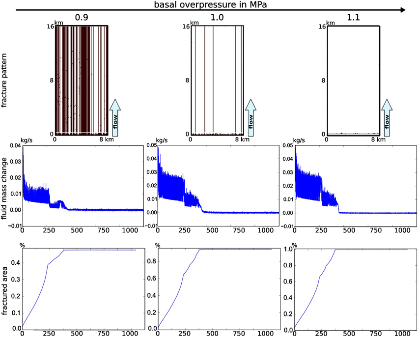
Figure 9. Final fracture pattern, fluid mass change (Δm_f/t) and total fractured area in % in experiments with vertical hydraulic fracture propagation at high solid viscosity ν = 10²³ Pa s. Fractured nodes are displayed in white. Most hydraulic fractures remain permanently open after their formation, and dynamic. Vertical clusters of hydraulic fractures, as under low viscosity conditions, do not occur, but continuous fractures develop connect between fluid source and surface. The vertical distribution of these fractures is determined by the Gaussian noise. Red line: From the marked time step onward the system is considered to be in a stable state. The power spectral density in Figure 11 is calculated for the stable region.

FIGURE 10

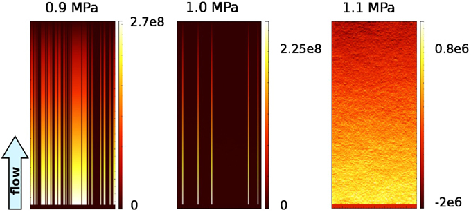
Figure 10. Effective stress field after equilibrium between fluid production and drainage is reached in vertical experiments with high viscosity ν = 10²³ Pa s. Fluid pathways are signified by lowered effective pressures.

Low Viscosity Simulations (Quick Fracture Healing)

Results for a viscosity mode (ν = 10¹⁷ Pa s) are displayed in Figure 6. At 0.85 MPa basal overpressure stationary hydraulic fractures form at locations with low tensile strength and propagate upwards from there. Although these fractures are spatially stationary, they are in a dynamic equilibrium as their tips open and close periodically.

Increasing the basal overpressure to 0.9 MPa leads to the formation of vertical mobile fracture clusters, which transport fluid pulses to the surface. The horizontal location of these vertical pathways is stationary and depends on the distribution of the tensile strength at the boundary layers between fluid source and non-fluid producing rock matrix. With increasing overpressure the horizontal width and the vertical extend of the fractured areas increase, and accordingly the total amount of fractured rock material. At a basal overpressure of approx. 1.8 MPa the system is completely fractured and fracture are stationary.

At the beginning of each low viscosity simulation fluid is transported by small mobile hydraulic fractures along distinct vertical pathways. These pathways are defined by the tensile strength at the interface between fluid source and rock matrix. These mobile fractures precede the fracture front and lead to permanent elevated fluid pressure along these vertical lines (Figure 7, right). Fractures propagate from both the surface, where effective stress is close to zero, and from the sink. With the onset of fracture formation at the surface in the more dynamic system with ν = 10¹⁷ Pa s, fluid is more efficiently drained and an intermediate plateau in the development of the fluid mass change with time Δm_f/t is reached.

It is not intuitively clear why fractures form far from the fluid source and close to the surface (Figure 7, left panel). The reason is the increase of the fluid pressure along the fluid pathways (Figure 7, right panel). This permanent increase, coupled with flow enabled by the background permeability of the material, leads occasionally to fracturing even if the fluid source is in a distance. This phenomenon affects primarily rocks at a shallow depth, because the necessary increase in fluid pressure is comparatively low.

The interplay of the fracture network with the stress field is visible in Figure 8, where the effective stress is displayed at a random time after the system reached the state of dynamic equilibrium. If hydraulic fractures form only along distinct vertical pathways (at a basal overpressure of 0.9 MPa), the effective stress along these pathways increases, potentially boosting formation of future fractures along these lines. Fractures close at locations where the effective stress is high (cp. Figure 8 at basal overpressure of 1.1 MPa).

High Viscosity Simulations (Slow Fracture Healing)

If the viscosity of the solid phase is increased to ν = 10²³ Pa s fracture patterns are near-stationary, regardless of the overpressure at the source. The stability of the fracture network results from relatively large time interval which is necessary to close these fractures in between fluid pulses (Figure 9). The effective stress field (Figure 10) is a function of the fracture pattern.

An intermediate plateau of Δm_f/t (approximately about 0.005–0.01 kg/s) is reached shortly before the fluid network is completed. This is similar to low viscosity simulations, but has a different reason: the plateau is reached once a first front of distinct hydraulic fractures reaches the surface. The interstitial spaces between these fractures function as propagation path for a secondary fracture front. Once this secondary fracture front reaches the surface, fluid production and fluid drainage reach a balanced state and Δm_f/t → 0.

Intermittency of Fluid Flow

If a signal is random can be distinguished by the power spectral distribution (“psd”). Figure 11 displays the psd calculated for the normalized fractured area of various simulations. The signal is typical of the forma f^−α, with α in the range 1.27–1.95, a clear sign that the signal is not random white noise, but shows a correlation in time.

FIGURE 11

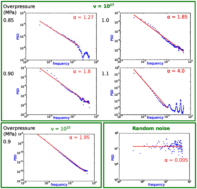
Figure 11. 1/f^α power spectral density (psd), calculated from the normalized fractured area in the simulations shown in Figures 6, 9 with Welch's method. α is calculated by linear regression for the near-linear intervals in the lower frequency band (red line). Not shown is the psd for systems where α = 0 (white noise), which was the case for ν = 10¹⁷/overpressure = 2.0 MPa, ν = 10¹⁷/1.0 MPa and ν = 10¹⁷/1.1 MPa (cp Figures 6, 9). For comparison the psd for a random time series (α = 0). The psd is close to 1/f if overpressure is small, α increases with increasing overpressure. The non-linearity at high frequencies of some simulations is probably related to the resolution and the simulation time.

In two cases the psd in the upper frequency band is non-linear. This affects simulations with a basal overpressures of 1.1/0.85 MPa and a viscosity ν = 10¹⁷. This result is most probably related to issues with relatively small spatial resolution or time intervals of the simulations. In these cases the α has been calculated for the linear part only. A value of α = 4.0 results for the linear region in the lower frequency band in case of the simulation with overpressure 1.1 MPa/ν = 10¹⁷, but this value can be attributed to the error.

Numerical simulations with near-stationary fracture networks develop α = 0, indicating constant values with some numerical random noise. This is the case in simulations where basal overpressure is relatively large (compare Figures 6, 9). Psd plots whith α = 0 were omitted from Figure 11.

The evolution of the fracture pattern for a particular simulation (with 0.9 MPa overpressure/ν = 10¹⁷) is shown in Figure 12. Figure 12A shows the vertical movement of fracture clusters in system snapshots from three consecutive years. When a cluster arrives at the surface fluid drainage occurs. The alternation with of fracture clusters with healed material causes the intermittency of the fluid flow. Figure 12B displays the time evolution of the fracture state of a horizontal section at 4000 m depth through a simulation. After c. 400 years the onset of a fracture pattern can be seen. From then on intermittent fracturing and healing occurs in almost regular intervals.

FIGURE 12

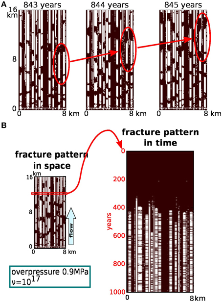
Figure 12. Time evolution of fracture clusters, demonstrated with the simulation using ν = 10¹⁷ and a basal overpressure of 0.9 MPa (see Figure 6). (A) Three subsequent snapshots of the fracture pattern. A single cluster is highlighted for clarity. Note the vertical movement at ~2000 m per year. (B) Time evolution of fractures in a 1D section through the simulation. Section line is marked by the red rectangle, located at 4000 m depth. Onset of the fracture/healing process after c. 300. The figure illustrates the intermittency of the fracture opening/healing process, which is induced by intermittent fluid flow.

Transport Efficiency of Fracture Networks

The efficiency of the fracture network to transport fluid can be characterized by the hydraulic conductivity over the total system length from source to sink, which will be termed the effective conductivity K_eff in the following. K_eff is calculated from Equation (1):

$K_{eff}=\frac{qL}{P_f^{source}-{\rho }_{H_{2}O}gL}.$

The resulting conductivity of the system in the stable state is plotted against the overpressure of the fluid source in Figure 13. Conductivity increases linearly with the fluid overpressure at the source layer until it reaches a constant maximum, starting at an overpressure of approx. 1 MPa (Figure 13), which is also the mean tensile strength of the material.

FIGURE 13

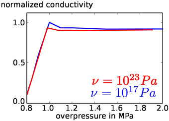
Figure 13. Effective conductivity of the total system between source and sink after equilibrium between fluid production and fluid drainage exists, drawn against various overpressure values for the basal layer. Red: slow fracture closure (ν = 10¹⁷ Pa s). Blue: fast fracture closure (ν = 10¹⁷ Pa s). To avoid scaling problems the conductivity has been normalized by the highest value of both plots. The development of the conductivity is almost identical, regardless of the viscosity and the dynamics of the fracture network.

This means that the mean efficiency of the fluid transport is independent of the fracture dynamics and the mobility of fractures. Even before equilibrium is reached, the efficiency of the different types of fracture networks in terms of fluid extraction from source to sink is similar (cp. the fluid mass change per time in Figures 6, 9). The main difference between static and dynamic fracture networks is the occurrence of fluid pulses in case of a dynamic fracture network, in difference to near-continuous flow in case of a stationary network.

Discussion

Dynamics of the Fracture Pattern

The development of dynamic fracture patterns in the computer simulations—in difference to a stable stationary fracture network—depends on the following three preconditions:

• The fluid overpressure is close to the mean tensile strength of the material, otherwise either no fractures form or the entire system fractures homogeneously,

• A fluid pressure gradient is present, as is the case in vertical profiles through the Earth's crust, and

• Fractures close quickly (i.e., the matrix viscosity is low), once the fluid pressure dropped below the solid pressure of the rock matrix.

The interface layer between the fluid source and the rock matrix is particularly important for the dynamics of the process. It works similar to a valve: once sufficient fluid migrated from the source into the adjacent rock mass, vertical hydraulic fractures nucleate and propagate toward the surface, thus transporting large amounts of fluid in a short period of time. Once the interface layer is sufficiently drained and the fluid pressure is lower than the matrix solid pressure, fractures close and the process starts again. This process leads to a non-random 1/f ^α type signal once the system reaches a state of dynamic equilibrium, with 1 < α < 2.

Preferred vertical fluid pathways develop according to the Gauss distribution at the interface. If a fracture closes, the fluid it transported is trapped and increases the local fluid pressure due to the very low matrix conductivity. The amount of additional fluid which is required to reactivate these nodes as fractures again is significantly smaller than in the adjacent material. These areas of heightened fluid pressure from potential future pathways for hydraulic fractures and quick fluid transport. Coupled with the non-destructive background diffusion of the fluid this can even lead to fracture initiation in a distance to the fluid source (Figure 6, left).

If the viscosity of the surrounding solid matrix is at 10²³ Pa s fracture closure is typically slower than pressure build up and hydraulic fracture patterns are stationary. Fluid mass balance is reached once the fracture network is capable of draining the entire fluid mass produced at the basal source. At this point the fractured area and the drained fluid mass converge to constant values, regardless of specific parameters. Periodic deviations from the equilibrium occur if ν is small, and are most significant at a slight overpressure of approx. 1.1–1.3 MPa.

Of particular interest to the dynamics of intermittent fluid flow are the amplitude and the frequency of fluid pulses. Pulses occur in simulations with a more dynamic low viscosity setting, visible in the rate of change of the fluid mass in the system (Figures 5, 8). The amplitude of fluid burst grows from low overpressure values till the overpressure is identical with the mean tensile stress is reached. A further increase of the fluid overpressure leads to the elimination of fluid bursts with small amplitudes, but still allows large fluid pulses in regular intervals.

Comparing the horizontal setup (without a fluid pressure gradient) to the results derived from vertical setups, it becomes clear that the fluid pressure gradient is essential for the development of dynamic fracture networks and fluid pulses.

The presented numerical method and simulations illustrate how a dynamic fluid flow system works, and the conditions under which they can efficiently transport large volumes of fluid to upper levels in the crust. These models are critical to understand highly complex transport systems, such as the ones responsible for the formation of large hydraulic breccias or dense networks of crack-seal veins.

The dynamics observed in the simulations—in particular the periodic changes of the fluid mass in the system, which was observed in most setups—might help to explain phenomena as the initially discussed hydraulic breccia, which depends on intermittent large scale fluid pulses.

It is of great interest to note that the efficiency of the fluid transport is virtually independent of the closing rate of the fractures. This means that velocity and dynamics of the fluid transport do not depend on the existence and reactivation of preexisting fracture networks, at least under model conditions. Potential fluid pathways are characterized by heightened local fluid pressure, which is a byproduct of previous fluid flow transport on fractures.

Summary and Conclusion

Fluid transport in the crust involves the formation of hydraulic fractures if the fluid overpressure at the source is sufficient. Geological evidence for this process exists, for instance in form of crack-seal veins or hydraulic breccias.

We simulated the dynamics of the vertical fluid flow from a fluid source with a constant overpressure to the surface, including the evolution of hydraulic fracture patterns. The ability to close fractures, once fluid pressure is lower than the solid pressure, is controlled by the matrix viscosity, which is taken to be at its uppermost and lowermost geologically realistic limits. The solid stress field is probably approximately accurate below 250 m depth, please note the discussion in Sections Fluid Flow and Hydraulic Fracturing in the Earth's Crust and General Setup.

Hydraulic fracture patterns may be either dynamic or stable, depending on the ability of fractures to close quickly, once the fluid pressure is released. In the dynamic case hydraulic fractures form mobile clusters and fluid transport occurs in periodic pulses. The reason is a valve function of the interface between fluid source and matrix rocks, where fluid pressure builds up by Darcian flow until it is sufficient to initiate fracture formation and quick removal of fluid mass toward the surface. The fracture dynamics follows a 1/f ^α pattern, with 1 < α < 2. If fractures heal slowly, the fracture network is stable and fluid flow is nearly constant.

The efficiency of the fluid transport is identical in both cases, regardless of the dynamics of the fracture network. While the dynamics of fluid flow and fracture formation differs considerably between the two settings, the efficiency of the fluid transport is not affected. Both systems have the same effective hydraulic conductivity. This is even more remarkable since the overpressure at the fluid source is constant, which means that the fluid production is entirely controlled by the efficiency of the transport mechanism. This means, in turn, that the existence of a stable fracture network is not as important as often assumed, as long as fluid overpressure is sufficient to initiate fracturing. More important than a fracture network are areas of heightened fluid pressure, where a relatively small amount of additional fluid is sufficient to initiate further fracturing. These areas are generally created by previous generations of hydraulic fracture swarms.

A key parameter for the dynamic fracture evolution is the presence of a fluid pressure gradient. In absence of a gradient fracture, as is the case of the “horizontal” setup, stable networks are being formed.

Conflict of Interest Statement

The authors declare that the research was conducted in the absence of any commercial or financial relationships that could be construed as a potential conflict of interest.

Acknowledgments

This study is carried out within the framework of DGMK (German Society for Petroleum and Coal Science and Technology) research project 718 “Mineral Vein Dynamics Modeling,” which is funded by the companies ExxonMobil Production Deutschland GmbH, GDF SUEZ E&P Deutschland GmbH, RWE Dea AG and Wintershall Holding GmbH, within the basic research programme of the WEG Wirtschaftsverband Erdöl- und Erdgasgewinnung e.V. We thank the companies for their financial support and their permission to publish our results.

We further acknowledge support by Deutsche Forschungsgemeinschaft and Open Access Publishing Fund of University of Tübingen.

References

1. Bons PD, Elburg MA, Gomez-Rivas E. A review of the formation of tectonic veins and their microstructures. J Struct Geol. (2012) 43:33–62. doi: 10.1016/j.jsg.2012.07.005

CrossRef Full Text | Google Scholar

2. Lazincka P. Breccias and ores. Part 1: history, organization and petrography of breccias. Ore Geol Rev. (1989) 4:315–44. doi: 10.1016/0169-1368(89)90009-7

CrossRef Full Text | Google Scholar

3. Lorilleux G, Jébrak M, Cuney M, Baudemont D. Polyphase hydrothermal breccias associated with unconformity-related uranium mineralization (Canada): from fractal analysis to structural significance. J Struct Geol. (2002) 24:323–38. doi: 10.1016/S0191-8141(01)00068-2

CrossRef Full Text | Google Scholar

4. Weisheit A, Bons PD, Elburg MA. Long-lived crustal-scale fluid flow: the hydrothermal mega-breccia of Hidden Valley, Mt. Painter Inlier, South Australia. Int J Earth Sci. (2013) 102:1219–36. doi: 10.1007/s00531-013-0875-7

CrossRef Full Text | Google Scholar

5. Jébrak M. Hydrothermal breccias in vein-type ore deposits: a review of mechanisms, morphology and size distribution. Ore Geol Rev. (1997) 12:111–34. doi: 10.1016/S0169-1368(97)00009-7

CrossRef Full Text | Google Scholar

6. Sibson R. Brecciation processes in fault zones—inferences from earthquake rupturing. Pure Appl Geophys. (1986) 124:159–75. doi: 10.1007/bf00875724

CrossRef Full Text | Google Scholar

7. Keulen N, Heilbronner R, Stunitz H, Boullier A-M, Ito H. Grain size distribution of fault rocks: a comparison between experimentally and naturally deformed granitoids. J Struct Geol. (2007) 29:1282–300. doi: 10.1016/j.jsg.2007.04.003

CrossRef Full Text | Google Scholar

8. Mort K, Woodcock NH. Quantifying fault breccia geometry: Dent Fault, NW England. J Struct Geol. (2008) 30:701–9. doi: 10.1016/j.jsg.2008.02.005

CrossRef Full Text | Google Scholar

9. Ramsay J. The crack-seal mechanism of rock deformation. Nature (1980) 284:135–9. doi: 10.1038/284135a0

CrossRef Full Text | Google Scholar

10. Koehn D, Passchier CW. Shear sense indicators in striped bedding-veins. J StructGeol. (2000) 22:1141–51. doi: 10.1016/S0191-8141(00)00028-6

CrossRef Full Text | Google Scholar

11. Lee YJ, Wiltschko DV. Fault controlled sequential vein dilation: competition between slip and precipitation rates in the Austin Chalk, Texas. J Struct Geol (2000) 22:1247–60. doi: 10.1016/S0191-8141(00)00045-6

CrossRef Full Text | Google Scholar

12. Laubach SE, Reed RM, Olson JE, Lander RH, Bonnell RM. Coevolution of crack-seal texture and fracture porosity in sedimentary rocks: cathodoluminescence observations of regional fractures. J Struct Geol. (2004) 26:967–82. doi: 10.1016/j.jsg.2003.08.019

CrossRef Full Text | Google Scholar

13. Renard F, Andréani M, Boullier AM, Labaume P. Crack-seal patterns: records of uncorrelated stress release variations in crustal rocks. Geol Soc Lond Spec Publ. (2005) 243:67–79. doi: 10.1144/GSL.SP.2005.243.01.07

CrossRef Full Text | Google Scholar

14. Yilmaz TI, Prosser G, Liotta D, Kruhl JH, Gilg HA. Repeated hydrothermal quartz crystallization and cataclasis in the Bavarian Pfahl shear zone (Germany). J Struct Geol (2014) 68:158–74. doi: 10.1016/j.jsg.2014.09.004

CrossRef Full Text | Google Scholar

15. Nunn JA. Buoyancy-driven propagation of isolated fluid-filled fractures: implication for fluid transport in Gulf of Mexico geopressured sediments. J Geophys Res. (1996) 101:2963–70. doi: 10.1029/95JB03210

CrossRef Full Text | Google Scholar

16. Dahm T. On the shape and velocity of fluid-filled fractures in the Earth. Geophys J Int. (2000) 142:181–92. doi: 10.1046/j.1365-246x.2000.00148.x

CrossRef Full Text | Google Scholar

17. Eichhubl P, Boles JR. Rates of fluid flow in fault systems-evidence for episodic rapid fluid flow in the Miocene Monterey Formation, coastal California. Am J Sci. (2000) 300:571–600. doi: 10.2475/ajs.300.7.571

CrossRef Full Text | Google Scholar

18. Okamoto A, Tsuchiya N. Velocity of vertical fluid ascent within vein-forming fractures. Geology (2009) 37:563–6. doi: 10.1130/G25680A.1

CrossRef Full Text | Google Scholar

19. Weisheit A, Bons PD, Danisik, M, Elburg MA. Crustal-scale folding: Palaeozoic deformation of the Mt Painter Inlier, South Australia. Geol Soc Lond Spec Publ. (2014) 394:53–77. doi: 10.1144/SP394.9

CrossRef Full Text | Google Scholar

20. Gomez-Rivas E, Bons PD, Koehn D, Urai JL, Arndt M, Virgo S, et al. The Jabal Akhdar Dome in the Oman Mountains: evolution of a dynamic fracture system. Am J Sci. (2014) 314:1104–39. doi: 10.2475/07.2014.02

CrossRef Full Text

21. Miller SA, Nur A. Permeability as a toggle switch in fluid-controlled crustal processes. Earth Planet Sci Lett. (2000) 183:133–46. doi: 10.1016/S0012-821X(00)00263-6

CrossRef Full Text | Google Scholar

22. Bons PD, van Milligen BP. New experiment to model self-organized critical transport and accumulation of melt and hydrocarbons from their source rocks. Geology (2001) 29:919–22. doi: 10.1130/0091-7613(2001)029<0919:NETMSO>2.0.CO;2

CrossRef Full Text | Google Scholar

23. Weertmann J. Theory of water-filled crevasses in glaciers applied to vertical magma transport beneath ocean ridges. J Geophys Res. (1971). 76:1171–83. doi: 10.1029/JB076i005p01171

CrossRef Full Text | Google Scholar

24. Oliver N, Rubenach M, Fu B, Baker J, Blenkinsop T, Cleverley J, et al. Granite-related overpressure and volatile release in the mid crust: fluidized breccias from the Cloncurry District, Australia. Geofluids (2006) 6:346–58. doi: 10.1111/j.1468-8123.2006.00155.x

CrossRef Full Text

25. Staude S, Bons PD, Markl G. Hydrothermal vein formation by extension-driven dewatering of the middle crust: an example from SW Germany. Earth Planet Sci Lett (2009) 286:387–95. doi: 10.1016/j.epsl.2009.07.012

CrossRef Full Text | Google Scholar

26. Bons PD, Fusswinkel T, Gomez-rivas E, Markl G, Wagner T, Walter B. Fluid mixing from below in unconformity-related hydrothermal ore deposits. Geology (2014) 42:1035–8. doi: 10.1130/G35708.1

CrossRef Full Text | Google Scholar

27. Vry J, Powell R, Golden KM, Petersen K. The role of exhumation in metamorphic dehydration and fluid production. Nat Geosci. (2010) 3:31–5. doi: 10.1038/ngeo699

CrossRef Full Text | Google Scholar

28. Matthäi SK, Heinrich CA., Driesner T. Is the Mount Isa copper deposit the product of forced brine convection in the footwall of a major reverse fault? Geology (2005) 32:357–360. doi: 10.1130/G20108.1

CrossRef Full Text | Google Scholar

29. Person M, Mulch A, Teyssler C, Gao Y. Isotope transport and exchange within metamorphic core complexes. Am J Sci. (2007) 307:555–89. doi: 10.2475/03.2007.01

CrossRef Full Text | Google Scholar

30. Papanastasiou PC. A coupled elastoplastic hydraulic fracturing model. Int J Rock Mech Min Sci. (1997) 34:240.e1–e15. doi: 10.1016/S1365-1609(97)00132-9

CrossRef Full Text | Google Scholar

31. Vychytil J, Horii H. Micromechanics-based continuum model for hydraulic fracturing of jointed rock masses during HDR stimulation. Mech Mater. (1998) 28:123–35. doi: 10.1016/S0167-6636(97)00061-6

CrossRef Full Text | Google Scholar

32. Hossain M, Rahman M. Numerical simulation of complex fracture growth during tight reservoir stimulation by hydraulic fracturing. J Petrol Sci Eng. (2008) 60:86–104. doi: 10.1016/j.petrol.2007.05.007

PubMed Abstract | CrossRef Full Text | Google Scholar

33. Ghani I, Koehn D, Toussaint R, Passchier CW. Dynamic development of hydrofracture. Pure Appl Geophys. (2013) 170:1685–703. doi: 10.1007/s00024-012-0637-7

CrossRef Full Text | Google Scholar

34. Ren L, Zhao J, Hu Y. Hydraulic fracture extending into network in shale: reviewing influence factors and their mechanism. Sci World J. (2014) 2014:1–9. doi: 10.1155/2014/847107

PubMed Abstract | CrossRef Full Text | Google Scholar

35. Hu Y, Chen G, Cheng W, Yang Z. Simulation of hydraulic fracturing in rock mass using a smeared crack model. Comput Struct. (2014) 137:72–77. doi: 10.1016/j.compstruc.2013.04.011

CrossRef Full Text | Google Scholar

36. Wang T, Zhou W, Chen J, Xiao X, Li Y, Zhao X. Simulation of hydraulic fracturing using particle flow method and application in a coal mine. Int J Coal Geol. (2014) 121:1–13. doi: 10.1016/j.coal.2013.10.012

CrossRef Full Text | Google Scholar

37. Connolly J, Podlachikov Y. Compaction-driven fluid flow in viscoelastic rock. Geodinamica Acta (1998) 11:55–84. doi: 10.1080/09853111.1998.11105311

CrossRef Full Text | Google Scholar

38. Connolly J, Podlachikov Y. A hydromechanical model for lower crustal fluid flow. In: Harlov DE, Austrheim, H. editors. Metasomatism and the Chemical Transformation of Rock. Berlin; Heidelberg: Springer Berlin Heidelberg (2013), pp. 599–658.

39. Hasenclever J, Theissen-Krah S, Rüpke H, Morgan J, Iyer K, Petersen S, et al. Hybrid shallow on-axis and deep off-axis hydrothermal circulation at fast-spreading ridges. Nature (2014) 508:508–12. doi: 10.1038/nature13174

PubMed Abstract | CrossRef Full Text

40. Gudmundsson A, Fjeldskaar I, Brenner SL. Propagation pathways and fluid transport of hydrofractures in jointed and layered rocks in geothermal fields. J Volcanol Geotherm Res. (2002) 116:257–78. doi: 10.1016/S0377-0273(02)00225-1

CrossRef Full Text | Google Scholar

41. Majer EL, Doe TW. Studying hydrofractures by high frequency seismic monitoring. Int J Rock Mech Min Sci Geomech Abstr. (1986) 23:185–199. doi: 10.1016/0148-9062(86)90965-4

PubMed Abstract | CrossRef Full Text | Google Scholar

42. Manger EG. Porosity and Bulk Density of Sedimentary Rocks. Washington, DC: United States Government Printing Office (1963).

Google Scholar

43. Singhal BBS, Gupta RP. Applied Hydrogeology of fractured Rocks. Dordrecht; Heidelberg; London; New York: Springer (2010). doi: 10.1007/978-90-481-8799-7

CrossRef Full Text | Google Scholar

44. Gudmundsson A. Rock Fractures in Geological Processes. Cambridge: Cambridge University Press (2011).

Google Scholar

45. Hering E, Martin R, Stohrer M. Physik für Ingenieure. Düsseldorf: VDI Verlag (1992).

Google Scholar

46. Fowler CMR. The Solid Earth: An Introduction to Global Geophysics. Cambridge: Cambridge University Press (2005). doi: 10.1029/90EO00309

CrossRef Full Text | Google Scholar

47. Sun C, Jin Z. Fracture Mechanics. Amsterdam: Elsevier (2012).

Google Scholar

48. Zhu Z. Evaluation of the range of horizontal stresses in the earth's upper crust by using a collinear crack model. J Appl Geophys. (2013) 88:114–21. doi: 10.1016/j.jappgeo.2012.10.007

CrossRef Full Text | Google Scholar

49. Fossen H. Structural Geology. Cambridge: Cambridge University Press (2010).

Google Scholar

50. Matthes S. Mineralogie. Berlin; Heidelberg: Springer (1996).

51. Maugis D. Contact, Adhesion, and Rupture of Elastic Solids. Berlin; Heidelberg: Springer (2000).

Google Scholar

52. Gölke M, Mechie J. Finite-element modelling of the structure and evolution of the South Kenya Rift, East Africa. Tectonophysics (1994) 236:439–452. doi: 10.1016/0040-1951(94)90188-0

CrossRef Full Text | Google Scholar

53. Wallner H, Schmeling H. Rift induced delamination of mantle lithosphere and crustal uplift: a new mechanism for explaining Rwenzori Mountains' extreme elevation? Int J Earth Sci. (2010) 99:1511–24. doi: 10.1007/s00531-010-0521-6

CrossRef Full Text | Google Scholar

54. Brace WF. Permeability of crystalline and argillaceous rocks. Int J Rock Mech Min Sci Geomech Abstr (1980) 17:241–51. doi: 10.1016/0148-9062(80)90807-4

CrossRef Full Text | Google Scholar

55. Owen P. Geological Fluid Dynamics Sub-surface Flow and Reactions. Cambridge: Cambridge University Press (2009).

Google Scholar

56. Stober I. Researchers study conductivity of crystalline rock in proposed radioactive waste site. Eos Trans Am Geophys Union (1996) 77:93. doi: 10.1029/96EO00062

CrossRef Full Text | Google Scholar

57. Preisig G, Eberhardt E, Gischig V, Roche V, van der Baan M, Valley B, et al. Development of connected permeability in massive crystalline rocks through hydraulic fracture propagation and shearing accompanying fluid injection. Geofluids (2015) 15: 321–37. doi: 10.1111/gfl.12097

CrossRef Full Text

58. Huffman A, Bowers G. Pressure Regimes in Sedimentary Basins and Their Prediction. Tulsa: The American Association of Petroleum and The Houston Chapter of The American Association of Drilling Engineers Geologists (2002).

Google Scholar

59. Zang A, Stephansson O. Stress Field of the Earth's Crust. Dordrecht: Springer (2010).

Google Scholar