Topological impact of constrained fracture growth

1. Introduction

Fluid transport in bedrock is of interest for a wide range of studies, from subsurface water reservoirs to exploitation of petroleum resources. Whether one aims at optimizing hydraulic fracturing, or to estimate flow in the bedrock, one wants a description of the bedrock which is as accurate as possible. An important part is the description of the fracture network, which plays an important part in fluid transport in geological media [1]. It is however impossible to detect the full fracture network. Information can be obtained through seismic or well logging, but this information has to be expanded with the use of a model to fully describe the network [2–4].

Since the transport properties of fracture networks are closely related to their topology, it is of great importance to be able to describe it quantitatively. Describing the topology of networks, or graphs, consisting of nodes and links, has been at the focal point of a huge research effort over the last 20 years [5, 6].

Fracture networks consist of intersecting sheetlike fractures — sheetlike since the fractures typically are very extended in two directions compared to the third. The ensuing networks have per se little to do with the graphs. Andresen et al. [7] proposed a transformation where the fracture sheets were represented by nodes and their intersections as links between them. This transformation is one-to-one and the resulting equivalent graphs give access to the plentiful and powerful tools that have been developed under the umbrella of modern network theory. Andresen et al. [7] went on to quantitatively compare fracture outcrops with a two-dimensional Discrete Fracture Network [8, 9] (DFN) model.

Andresen et al. [7] found fracture outcrops to form disassortative networks, that is fractures tend to connect to fractures with different degree, while the DFN model resulted in assortative networks where fractures tended to be connected with fractures of similar degree.

A noteworthy simplification in the DFN model studied by Andresen et al. [7] is that the fractures are placed independently of each other and that they are free to cross each other. An improvement of the DFN model has been based on the idea that large fractures can stop the propagation of smaller fractures [3]. This mechanical DFN model is based on simplified mechanical rules which produce a fracture network formation that includes fracture nucleation, growth and arrest [3]. For three-dimensional models, the mechanical DFN model has been shown to give much higher flow channeling than the Poissonian DFN model [10].

This paper presents a topological analysis of both two- and three-dimensional fracture networks based on the transformation proposed by Andresen et al. [7] to evaluate the impact of the constrained fracture growth in the mechanical DFN model compared to the Poissonian DFN model. The two-dimensional models are also compared against the outcrops studied by Andresen et al. [7].

Ideally, the results presented in the paper should have been compared to measured three-dimensional fracture networks. Unfortunately, no data set of sufficient quality exists that makes this possible. There are, however, other systems where a comparison between model and nature is possible. For example, the mineral desert rose consists of intersecting sheetlike crystals. Recently, an analysis of this system has been presented, see Hope et al. [11]. Another system where a comparison should be possible is slow drainage in layered porous media which produces multiple sheetlike structures. A model exists [12], but to our knowledge no experimental results have been produced so far. In this case, data of sufficient quality should be obtainable.

Both the Poissonian and mechanical DFN models are found to generate networks, in both two and three dimensions, that transform into small-world graphs. The models are found to differ when it comes to degree mixing. For two dimensions, the Poissonian model is found to be assortative, while the mechanical model is disassortative. In three dimensions both models are found to be disassortative, and the difference between the models is limited to the strength of the disassortative mixing. As such the two-dimensional model is found to reproduce the disassortative degree mixing found by Andresen et al. [7] for the outcrop data. However, it should be noted that there is individual differences between the outcrops, and their general classification as disassortative is uncertain.

There is also a difference between the networks generated in two and three dimensions with respect to the size of the largest component in the network. In three dimensions the models tend to generate well connected networks where the largest component make up a larger part of the network, for the Poissonian model this differs from the situation in two dimensions.

This article is structured as follows. Section 2 presents the DFN models before the basis for the network analysis is presented in Section 3. Results are presented and discussed in Section 4 before concluding remarks are drawn in Section 5.

2. Discrete Fracture Network Model

Most fractured reservoirs can only be given a statistical description. A common method of introducing such a description when investigating flow properties of geological sites is to use the consecutive stochastic, or Poissonian DFN model [1, 8, 13]. Generally, DFN models do not use the mechanical relation between fractures. However, distribution of fracture intersections and flow channeling are critical parameters in the hydraulic properties of the fractured reservoirs. Both aspects are likely related to spatial correlations and interactions between fractures [14]. The capacity of DFN models to reproduce flow channeling is essential for a good estimation of hydraulic properties [15–17].

The Poissonian DFN model generally does not produce T-shaped intersections where a fracture terminates at another fracture. Instead the model creates X-shaped intersections since the fractures are free to cross each other. This could be addressed by integration of simplified mechanical rules to take into account the fracture interaction and their consequences on the distribution of intersection and spatial organization of the network fracture [3, 18–20]. Building on simplified mechanical rules Davy et al. have introduced a mechanical DFN model [3, 20].

2.1. Poissonian DFN Model

Orientation, position and length or diameter the fractures are assigned independently in the Poissonian DFN model [21, 22], and the properties of any fracture is blind to all other fractures.

The fracture length distribution is a critical parameter in controlling connectivity and permeability [23, 24]. Observations of fracture traces in outcrops show that fracture lengths follow power-laws [25, 26].

$\begin{array}{ll}p(l)~l^{-{\alpha }_l}.& (1)\end{array}$

From observations and mechanical/geometrical arguments, Davy et al. [20] suggest that the power-law exponent should tend to the self-similar case at large fracture lengths, which fixes the exponent α_l to 4 for three-dimensional networks.

For this paper the model is considered in the most simplified form. The fracture centers are randomly distributed, given a fracture density. The orientation of each fracture is drawn from a uniform random distribution. Hence, no assumptions are made with respect to the stress field direction that has generated the fractures.

2.2. Mechanical DFN Model

In the mechanical DFN model, the generation of the fracture networks occurs in three steps; fracture nucleation, fracture growth and fracture arrest [3].

Nucleation gives the fractures an initial position as well as an orientation. As in the Poissonian model, the position is random and no preferential orientation is assumed. Nucleation centers are randomly generated at a rate

$\begin{array}{ll}{ṅ}_N=\frac{d{n}_N}{dt},& (2)\end{array}$

where n_N is the number of nuclei, and t the time [3].

Once created, a fracture grows at a rate given by

$\begin{array}{ll}\frac{dl}{dt}=G{l}^a,& (3)\end{array}$

where l is the fracture length or diameter, G the growth rate and a the growth exponent [3].

Arrest of a fracture is caused by the fracture growth being hindered by mechanical interactions with other fractures. This occurs when a fracture gets close to a larger fracture and a simplified arrest rule prevents fractures from crossing larger fractures. This imitates the interaction between real fractures and results in a self-similar power-law distribution of fracture sizes [3, 20].

The ratio G∕ṅ_N can be used to separate between two different versions of the mechanical model [10]. If G ≫ ṅ_N the time for a fracture to grow is short compared to the time between the appearance of successive nuclei. Thus, fractures grow one by one in a sequential mode [10]. On the other hand, if G ≪ ṅ_N fractures will grow simultaneously in a competitive mode [10].

The two models will have different structures since the ratio of X-type and T-type intersections will depend on whether the fractures grow sequentially or not [10].

The mechanical model can also make use of two different stop criteria. When a fracture meets a larger fracture the smallest fracture can stop completely (mode A) or it can be free to grow in the opposite direction (mode B) up to the point when it meets another large fracture [3].

2.3. Compared Models

In the present study, topology is compared for both competitive (C) and sequential (S) mechanical models for both mode A and mode B stop criteria. Hence, the mechanical DFN model should be studied in four different limits; C or S and A or B. For each model, the eventual fracture density is different.

As a comparison to the mechanical models, the Poissonian DFN model has been generated for two different fracture densities, based on the maximum and minimum densities from the mechanical model. The high density case (P-H-D) has the same density as (M-C-B), while the low density case (P-L-D) is similar in density to (M-A-S).

3. Network Analysis

Transforming the fracture network into a graph is done as suggested by Andresen et al. [7]. As shown in Figures 1 and 2, each fracture is defined as a node and nodes are linked if they represent intersecting fractures.

FIGURE 1

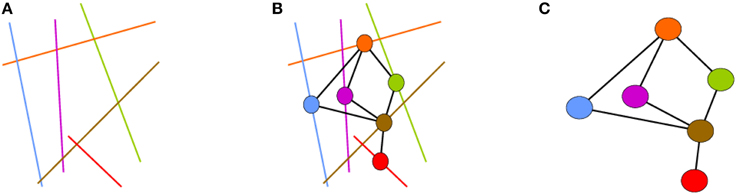
Figure 1. (A) Representation of a two-dimensional fracture network. (B) Equivalent graph placed on top of fracture network. (C) Equivalent graph representation of (A). (Figure from Andresen et al. [7].)

FIGURE 2

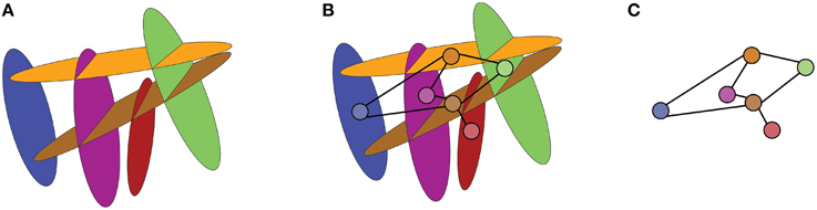
Figure 2. (A) Representation of a three-dimensional fracture network. (B) Equivalent graph placed on top of fracture network. (C) Equivalent graph representation of (A).

To evaluate the properties of a graph, it is useful to compare against randomized versions of the same graph [6]. For this purpose two randomized versions of each of the graphs are made. The first is a completely random model with the same number of nodes and links as the original graph [27], while the second is a rewired version of the original graph which preserves the degree of each node, but randomizes which nodes that are connected [28].

Clustering, C, is a measure of the local connectivity of a graph. For a specific node the coefficient, C_i, gives the ratio between the number of connections between the k_i neighbors of node i and the k_i(k_i − 1) ∕ 2 possible ways they could be connected [29, 30]. In terms of the original fracture network, the number of connections, or degree, of a given node k_i in the graph is the number of fractures that intersect the fracture represented by the node.

The average over the clustering coefficients of all nodes gives a measure of the clustering in the entire graph and can be expressed as

$\begin{array}{ll}C=\frac{1}{N}{\displaystyle \sum _{i=1}^N}{C}_i=\frac{1}{N}{\displaystyle \sum _{i=1}^N}\frac{2K_i}{k_i(k_i-1)}.& (4)\end{array}$

where N is the number of nodes in the graph and K_i is the number of connections between node i's neighbors [30].

In the case where a node has less than two neighbors, the local clustering coefficient is defined to be zero [31].

Efficiency, E, is a measure of the long range connectivity of a network. High efficiency indicates that one can expect to go from a given fracture to any other fracture without having to go through many intermediate fractures. Given all possible paths between nodes i and j the shortest path, d_ij, is found based on the fewest number of links traversed. The efficiency can then be defined as [32, 33]

$\begin{array}{ll}E=\frac{1}{N(N-1)}{\displaystyle \sum _{(i,j)\in N,i\ne j}}\frac{1}{d_{ij}}.& (5)\end{array}$

In the case were nodes i and j are unconnected d_ij = ∞ [32].

A measure of degree mixing is the assortativity coefficient r, which for a graph with M links can be expressed as follows [34]

$\begin{array}{cc}r=\frac{M^{-1}{\displaystyle {\sum }_i{k}_{1i}{k}_{2i}}-{[M^{-1}{\displaystyle {\sum }_i\frac{1}{2}(k_{1i}+k_{2i})}]}^2}{M^{-1}{\displaystyle {\sum }_i\frac{1}{2}(k_{1i}{}^2+k_{2i}{}^2)}-{[M^{-1}{\displaystyle {\sum }_i\frac{1}{2}(k_{1i}+k_{2i})}]}^2},& \left(6\right)\end{array}$

where k_1i and k_2i are the degrees of the nodes linked by the ith link. Assortative mixing is indicated by r > 0, while r < 0 indicates disassortative mixing.

An estimate of the variance of the assortative coefficient for a single sample can be found using the jackknife estimate

$\begin{array}{ll}{\sigma }_j^2=\frac{M-1}{M}{\displaystyle \sum _{i=1}^M}{\left[r_i-r\right]}^2,& (7)\end{array}$

where M is the number of links in the network and r_i is the assortative coefficient when excluding the ith link in the calculation [31, 35].

Community detection identifies parts of the network which are highly interconnected but have relatively few connections to other parts of the network. What is found to constitute a community structure will depend on the algorithm used as well as the number of communities one divide the network into [6]. This work make use of the Girvan-Newman algorithm [36]. The number of communities is chosen to maximize modularity, Q. The modularity measures the fraction of links in a network that connects nodes of the same type minus the expected value for a network with the same community divisions but with random connections between the nodes [37]. If the number of links within the communities is not higher than in the random case random, then Q = 0, while Q = 1 is the maximum limit for extremely strong community structure [37]. Newman and Girvan report that typical values for networks with strong community structure are in the range from 0.3 to 0.7 and that higher values are rare [37].

4. Results and Discussion

As was to be expected, the stop criteria in the two limits of the mechanical models has a significant impact on the ratio between links and nodes in the corresponding graphs, as well as degree distribution (as shown in Tables 1, 2 and Figures 3, 4). This is caused by the higher number of connections in the mode B versions of the models resulting from the fact that fractures are only arrested in the direction where they intersect larger fractures. With regard to the ratio between links and nodes the two mechanical models with stop criterion B have a much higher number of links than nodes. However, the mechanical model with stop criterion A results in either a similar number of nodes and links (M-C-A) or a higher number of nodes than links (M-S-A). As such the mechanical model offers a large diversity when it comes to the number of intersections per fracture. It should be noted that there is a difference between two-dimensional and three-dimensional networks and as seen in Tables 1, 2, the number of links in the Poissonian model is much closer to the number of nodes in two dimensions than what is the case for three dimensions. For the low density case in two dimensions, the Poissonian model in fact shows fewer links than nodes.

TABLE 1

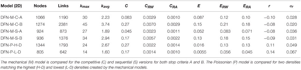
Table 1. Averaged values of the number of nodes, links, maximum degree k_max, average degree k_avg, clustering coefficient C, clustering coefficient for rewired graphs C_RW, clustering coefficient for random graphs C_RA, efficiency E, efficiency for rewired graphs E_RW, efficiency for random graphs E_RA, assortativity coefficient r with its standard deviation σ_r for 50 samples of each of the different limits of the two DFN models in two dimensions.

TABLE 2

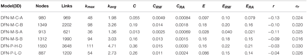
Table 2. Averaged values of the number of nodes, links, maximum degree k_max, average degree k_avg, clustering coefficient C, clustering coefficient for rewired graphs C_RW, clustering coefficient for random graphs C_RA, efficiency E, efficiency for rewired graphs E_RW, efficiency for random graphs E_RA, assortativity coefficient r with its standard deviation σ_r for 50 samples of each of the different limits of the two DFN models in three dimensions.

FIGURE 3

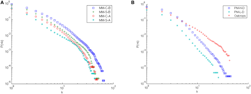
Figure 3. Cumulative degree distribution for the two-dimensional DFN models. Results are based on 50 samples of each model. (A) Results for the mechanical model in all limits. (B) Results for the Poissonian model in both limits as well as for the outcrops.

FIGURE 4

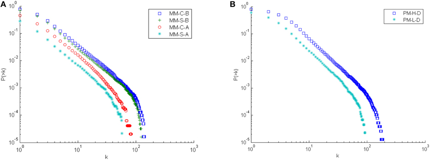
Figure 4. Cumulative degree distribution for the three-dimensional DFN models. Results are based on 50 samples of each model. (A) Results for the mechanical model in all limits. (B) Results for the Poissonian model in both limits.

The difference in the stop criteria also has an impact on clustering, which is up to an order of magnitude higher in the mode B cases. However, when comparing the clustering against rewired and random versions of the networks, all models, mechanical and Poissonian, are similar in having clustering much higher than in their randomized versions. Broadly speaking, the clustering is an order of magnitude higher than the closest of the randomized networks (as shown in Tables 1, 2). With an efficiency of the same order as the randomized network, this indicates that all models form small-world networks [29, 33]. This is consistent with previous results for both DFN models and outcrops by Andresen et al. [7].

With regard to the degree distribution for the three-dimensional models, Figure 4 shows similar results for the competitive and sequential models when stop criterion B is used, but that the models differ when making use of stop criterion A. Sequential and competitive models differ both when it comes to density and ratio of X- and T- intersections. The sequential model with stop criteria A differs from the others and is close to critical organization with both low density and high number of T-intersections.

It should be noted that connectivity increases with increasing dimensionality. This is e.g. illustrated by the site percolation threshold being around 0.592 for the square lattice and 0.246 for the cubic lattice [38].

The main difference between the DFN model and the outcrops found by Andresen et al. was in the degree mixing [7]. While the DFN model resulted in assortative mixing, the outcrops resulted in disassortative mixing. The analysis of the mechanical DFN model shows disassortative mixing, as shown in Tables 1, 2, indicating that the limitations on fracture propagation have a significant impact on the degree mixing.

This is consistent with a previous study of fractures in sea ice by Vevatne et al. where it was shown that a simple growing fracture network model could produce disassortative mixing if existing fractures could stop the propagation of fractures growing into them [39]. In the model by Vevatne et al. the fractures ability to arrest intersecting fractures was a fixed probability, equal for all fractures [39].

The assortative coefficient indicates a clear difference between the two-dimensional models. While all limits of the mechanical model result in disassortative networks, the Poissonian model results in assortative networks. For three-dimensional networks all models result in disassortative networks and the difference between the models is limited to the mechanical model showing stronger disassortative mixing than the Poissonian model.

Another noticeable difference between the two-dimensional and three-dimensional DFN models is the size of the largest component. With the exception of the mechanical DFN model in the (M-S-A) limit where the largest component only makes up 40 % of the nodes in the graph, all three-dimensional models appear, as shown in Table 3, to be highly connected with the largest component making up from 69 to 92 % of the network. The mechanical model is still well connected in two dimensions, as shown in Table 4, but the Poissonian model results in the largest component making up only 7–28 % of the network. Comparing the two-dimensional models to the outcrops, indicates that the mechanical model is closest, but that the model is too connected.

TABLE 3

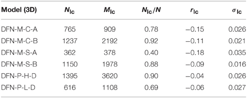
Table 3. Average values for number of nodes N_lc, links M_lc, average ratio of nodes in the largest component and the entire graph N_lc∕N, as well as assortativity coefficient r_lc with its standard deviation σ_lc, for the largest component for 50 samples of each of the different limits of the two DFN models in three dimensions.

TABLE 4

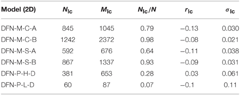
Table 4. Average values for number of nodes N_lc, links M_lc, average ratio of nodes in the largest component and the entire graph N_lc∕N, as well as assortativity coefficient r_lc with its standard deviation σ_lc, for the largest component for 50 samples of each of the different limits of the two DFN models in two dimensions.

The networks generated by the DFN models are compared against the same outcrops which Andresen et al. [7] used in their topological comparison. The outcrops are from two locations on the Swedish south-east coast, namely Simpevarp and Laxemar [40, 41]. The outcrops cover between 215 and 524 m² and all visible fractures with length over 0.5 m have been recorded [40, 41]. Detailed descriptions of the bedrock composition and geological history are given in Hermanson et al. [40, 41] and Strøm et al. [42].

The average assortativity coefficient of the outcrops is found to be r = −0.02 with σ_r = 0.058. The individual samples span, as shown in Table 5, from r = −0.11 to r = 0.05 and weakens the general conclusion of disassortative outcrops. An overview of the assortativity coefficient for all outcrops and their largest components are given in Table 5. Further studies of more outcrops could clarify the question of the degree mixing behavior in outcrops.

TABLE 5

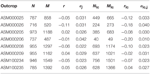
Table 5. Number of nodes N, links M, assortativity coefficient r with its jackknife-based standard deviation σ_j, and the same for the largest component (lc) for each outcrop.

As shown in Figures 5, 6 both models and the outcrops show a strong correlation between degree and fracture length. As such the difference in degree mixing is closely related to whether fractures intersect fractures of similar or dissimilar length. The stop criteria clearly separates the mechanical models and the use of stop criterion B, as expected, generate fractures with more intersections than the models using stop criterion A. In addition, the area belonging to a fracture of a given degree tends to be larger for the models using stop criterion A, than for the models using criterion B, reflecting density differences between the models.

FIGURE 5

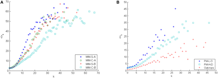
Figure 5. Averaging the area for all fractures with similar degree shows a clear connection between length and degree. Results are based on 50 samples of each two-dimensional DFN model. (A) Results for the mechanical model in all limits. (B) Results for the Poissonian model in both limits as well as the outcrops.

FIGURE 6

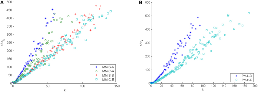
Figure 6. Averaging the area for all fractures with similar degree shows a clear connection between area and degree. Results are based on 50 samples of each three-dimensional DFN model. (A) Results for the mechanical model in all limits. (B) Results for the Poissonian model in both limits.

The difference between networks displaying assortative degree mixing and those displaying disassortative degree mixing has been attributed to the existence of communities with strong internal connectivity in assortative networks [43]. However, the presence of community structure also in disassortative networks has been suggested by Radicchi et al. [44]. To investigate the community structure of the fracture networks, the analysis is limited to the largest component of each of the two-dimensional networks.

It is noted that the largest clusters generally are more disassortative than the whole samples. In fact the average assortativity coefficient for the largest cluster in each sample of the two-dimensional Poissonian DFN model in the low density case shows disassortative mixing, as shown in Table 4. The largest component in the two-dimensional Poissonian DFN model however, makes up a relative small part of the network.

As shown in Figures 7, 8, the existence of community structure is not limited to the assortative networks, but also exist in the disassortative networks.

FIGURE 7

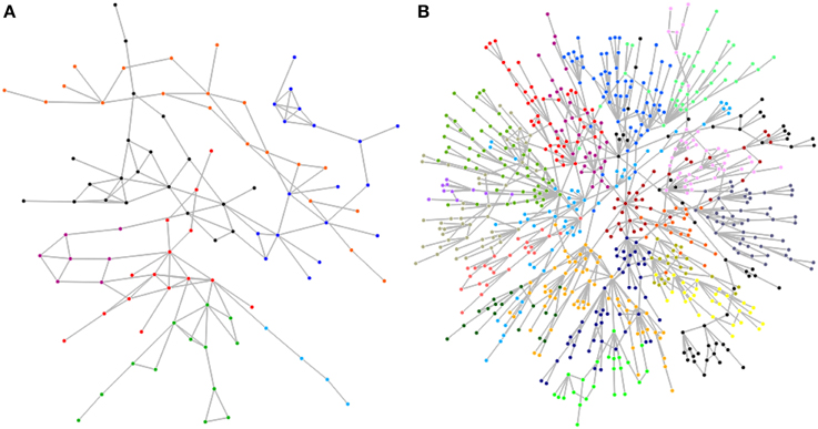
Figure 7. (A) Community structure of the largest component (r = 0.12) of a sample of the Poissonian DFN model shows seven distinct groups. (B) Community structure of the largest component (r = −0.18) of a sample of the mechanical DFN model shows 20 distinct groups. The different groups or communities are identified by the color of the nodes.

FIGURE 8

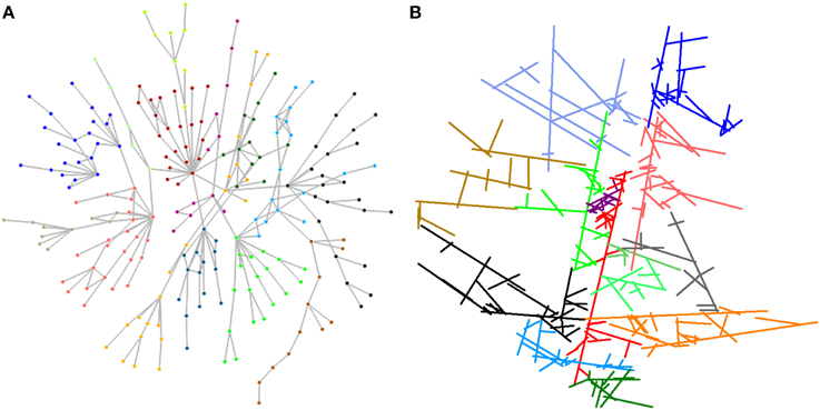
Figure 8. (A) Community structure of the largest component (r = −0.18) of outcrop ASM000026 shows 14 distinct groups. (B) The groups in (A) plotted as they are positioned in the fracture network.

Figure 7 shows the community structure of the largest component in samples of the Poissonian DFN model and the mechanical DFN model. The component from the Poissonian model has an assortativity coefficient of r = 0.12 and when divided into communities by maximize modularity, it shows 7 different groups and a resulting modularity of Q = 0.69. The component from the mechanical DFN model has an assortativity coefficient of r = −0.18 and shows a community structure with 20 different groups and corresponding modularity of Q = 0.86.

The most disassortative outcrop, ASM000026, has an assortativity coefficient of r = −0.18 for the largest component. However, as shown in Figure 8 a strong community structure is found with 14 different groups and a modularity as high as Q = 0.84.

Even though a clear community structure is found for both the assortative and disassortative networks, there are clear differences between them. While the number of nodes in the largest components is a dominant difference as shown in Figure 7, it is also worth noticing the tree-structure for both disassortative samples (Figures 7B, 8A). While there are few links between the communities, the tree-structure shows that there are relatively few interconnections in the communities as well.

The low number of links connecting the different communities results, as illustrated in Figure 8B, in a few fractures being the only connections between different parts of the network. As such, these few fractures are the only flow channels between their community and the connected communities.

As they are likely to be important flow channels, the largest fractures are of special interest. When looking at how the ten largest fractures connect to each other in the three-dimensional model, there is trend for the number of connection to increase with density and for the variants of the Poissonian DFN model to show more connections between these fractures than the variants of the mechanical DFN model do. The least dense of the mechanical DFN models (S-A) typically does not show connections between the largest fractures, while the densest version (C-B) typically shows that the longest fractures connect to one of the other longest fractures. This is comparable to the low density case for the Poissonian model, while the high density case shows the longest fractures linking on average to 1.5 of the other longest fractures. The Poissonian model could probably approach the mechanical model on this point by the introduction of a correlation between fracture length and orientation.

5. Conclusion

The mechanical DFN model, and its implementation of fractures acting as barriers for smaller fractures, has significant impact on the topology of the generated fracture networks. For two-dimensional fracture networks the mechanical DFN model, independent of the limit used, generates disassortative degree mixing, while the Poissonian model generates assortative degree mixing. For three-dimensional fracture networks there is also a clear separation between the different limits of the mechanical DFN model on one hand, and their Poissonian counterparts on the other hand. However, in three dimensions both models generate disassortative networks, and the difference is limited to the strength of the disassortative mixing.

The assortativity coefficient for the outcrops shows individual differences between the samples when it comes to whether they are assortative or disassortative, with the average leaning toward disassortative. Further study of more samples could clarify the matter.

The Poissonian model in its two limits tends to be much more connected in three dimensions than in two dimensions. This results in the largest component making up a much larger part of the network in the three-dimensional case than in the two-dimensional case. Comparing the two-dimensional models to the outcrops shows that the mechanical model is the closest, but that the model is too connected. This could possibly be addressed by introducing a threshold of available energy for each fracture so that fractures could stop propagating even if they do not meet other fractures.

The difference between the Poissonian and mechanical DFN models in how the fractures connect is likely to have an impact on the flow properties of the networks. The existence of such differences has been identified by Maillot et al. [10] who showed that the mechanical DFN model in the different limits results in more flow channeling, or localization of the flow, than the Poissonian DFN model.

Author Contributions

SH performed the network analysis and wrote the first version of the paper. PD and JM contributed the DFN data and to the presentation of the DFN models. PD and RL contributed to elaborating the DFN mechanical model. PD and AH took part in discussions and in writing the paper.

Conflict of Interest Statement

The authors declare that the research was conducted in the absence of any commercial or financial relationships that could be construed as a potential conflict of interest.

Acknowledgments

The authors thank Svensk Kärnbränslehantering AB for outcrop data and MIT Strategic Engineering for making their Matlab Tools for Network Analysis publicly available. SH and AH thank Norges Forskningsråd for funding through the CLIMIT program (grant no. 199970) and the RENERGI program (grant no. 217413/E20).

References

1. Berkowitz B. Characterizing flow and transport in fractured geological media: a review. Adv Water Resour. (2002) 25:861–84. doi: 10.1016/S0309-1708(02)00042-8

CrossRef Full Text | Google Scholar

2. Sausse J, Dezayes C, Dorbath L, Genter A, Place J. 3D model of fracture zones at Soultz-sous-Forêts based on geological data, image logs, induced microseismicity and vertical seismic profiles. C R Geosci. (2010) 342:531–45. doi: 10.1016/j.crte.2010.01.011

CrossRef Full Text | Google Scholar

3. Davy P, Le Goc R, Darcel C. A model of fracture nucleation, growth and arrest, and consequences for fracture density and scaling. J Geophys Res Solid Earth (2013) 118:1393–407. doi: 10.1002/jgrb.50120

CrossRef Full Text | Google Scholar

4. McClure MW, Horne RN. Discrete Fracture Network Modeling of Hydraulic Stimulation. New York, NY: Springer (2013). doi: 10.1007/978-3-319-00383-2

CrossRef Full Text | Google Scholar

5. Barabási AL. Linked. New York, NY: Plume (2003).

Google Scholar

6. Newman MEJ. Networks: An Introduction. Oxford: Oxford University Press (2010). doi: 10.1093/acprof:oso/9780199206650.001.0001

CrossRef Full Text | Google Scholar

7. Andresen CA, Le Goc R, Davy P, Hansen A, Hope SM. Topology of fracture networks. Front Phys. (2013) 1:7. doi: 10.3389/fphy.2013.00007

CrossRef Full Text | Google Scholar

8. Jing L, Stephansson O. Fundamentals of Discrete Element Methods for Rock Engineering. Amsterdam: Elsevier (2007).

Google Scholar

9. Davy P, Bour O, de Dreuzy JR, Darcel C. Flow in multiscale fractal fracture networks. In: Cello G, Malamud BD, editors. Fractal Analysis for Natural Hazards. Vol. 261. London: Geological Society (2006). pp. 31–45. doi: 10.1144/gsl.sp.2006.261.01.03

CrossRef Full Text

10. Maillot J, Davy P, de Dreuzy JR, Le Goc R, Darcel C, Stigsson M. Comparison between “Poissonian” and “mechanically-oriented” DFN models for the prediction of permeability and flow channeling. In: International Conference on Discrete Fracture Network Engineering. Vancouver, BC (2014). p. 114.

Google Scholar

11. Hope SM, Kundu S, Roy C, Manna SS, Hansen A. Network topology of the desert rose. Front Phys. (2015) 3:72. doi: 10.3389/fphy.2015.00072

CrossRef Full Text | Google Scholar

12. Parteli EJR, da Silva LR, Andrade JS. Self-organized percolation in multi-layered structures. J Stat Mech Theory Exp. (2010) 2010:P03026. doi: 10.1088/1742-5468/2010/03/P03026

CrossRef Full Text | Google Scholar

13. Neuman SP. Trends, prospects and challenges in quantifying flow and transport through fractured rocks. Hydrogeol J. (2005) 13:124–47. doi: 10.1007/s10040-004-0397-2

CrossRef Full Text | Google Scholar

14. Oron AP, Berkowitz B. Flow in rock fractures: the local cubic law assumption reexamined. Water Resour Res. (1998) 34:2811–25. doi: 10.1029/98WR02285

CrossRef Full Text | Google Scholar

15. Ronayne MJ, Gorelick SM. Effective permeability of porous media containing branching channel networks. Phys Rev E (2006) 73:026305. doi: 10.1103/PhysRevE.73.026305

PubMed Abstract | CrossRef Full Text | Google Scholar

16. Trinchero P, Sánchez-Vila X, Fernàndez-Garcia D. Point-to-point connectivity, an abstract concept or a key issue for risk assessment studies? Adv Water Resour. (2008) 31:1742–53. doi: 10.1016/j.advwatres.2008.09.001

PubMed Abstract | CrossRef Full Text | Google Scholar

17. Kerrou J, Renard P, Franssen HJH, Lunati I. Issues in characterizing heterogeneity and connectivity in non-multiGaussian media. Adv Water Resour. (2008) 31:147–59. doi: 10.1016/j.advwatres.2007.07.002

CrossRef Full Text | Google Scholar

18. Cacas MC, Daniel JM, Letouzey J. Nested geological modelling of naturally fractured reservoirs. Petrol Geosci. (2001) 7:S43–52. doi: 10.1144/petgeo.7.S.S43

CrossRef Full Text | Google Scholar

19. Josnin JY, Jourde H, Fénart P, Bidaux P. A three-dimensional model to simulate joint networks in layered rocks. Can J Earth Sci. (2002) 39:1443–55. doi: 10.1139/e02-043

CrossRef Full Text | Google Scholar

20. Davy P, Le Goc R, Darcel C, Bour O, de Dreuzy JR, Munier R. A likely universal model of fracture scaling and its consequence for crustal hydromechanics. J Geophys Res Solid Earth (2010) 115:411. doi: 10.1029/2009JB007043

CrossRef Full Text | Google Scholar

21. Darcel C, Bour O, Davy P, de Dreuzy JR. Connectivity properties of two-dimensional fracture networks with stochastic fractal correlation. Water Resour Res. (2003) 39:1272. doi: 10.1029/2002wr001628

CrossRef Full Text | Google Scholar

22. de Dreuzy JR, Méheust Y, Pichot G. Influence of fracture scale heterogeneity on the flow properties of three-dimensional discrete fracture networks (DFN). J Geophys Res Solid Earth (2012) 117:B11207. doi: 10.1029/2012jb009461

CrossRef Full Text | Google Scholar

23. Bour O, Davy P. On the connectivity of three-dimensional fault networks. Water Resour Res. (1998) 34:2611–22. doi: 10.1029/98WR01861

PubMed Abstract | CrossRef Full Text | Google Scholar

24. de Dreuzy JR, Davy P, Bour O. Percolation parameter and percolation-threshold estimates for three-dimensional random ellipses with widely scattered distributions of eccentricity and size. Phys Rev E (2000) 62:5948–52. doi: 10.1103/PhysRevE.62.5948

PubMed Abstract | CrossRef Full Text | Google Scholar

25. Renshaw CE. Connectivity of joint networks with power law length distributions. Water Resour Res. (1999) 35:2661–70. doi: 10.1029/1999WR900170

CrossRef Full Text | Google Scholar

26. Bonnet E, Bour O, Odling NE, Davy P. Scaling of fracture systems in geological data. Rev Geophys. (2001)39:347–83. doi: 10.1029/1999RG000074

PubMed Abstract | CrossRef Full Text | Google Scholar

27. Erdős P, Rényi A. On random graphs i. Publ Math. (1959) 6:290–7.

PubMed Abstract

28. Maslov S, Sneppen K. Specificity and stability in topology of protein networks. Science (2002) 296:910–3. doi: 10.1126/science.1065103

PubMed Abstract | CrossRef Full Text | Google Scholar

29. Watts DJ, Strogatz SH. Collective dynamics of ‘small-world’ networks. Nature (1998) 393:440–2. doi: 10.1038/30918

PubMed Abstract | CrossRef Full Text | Google Scholar

30. Albert R, Barabási AL. Statistical mechanics of complex networks. Rev Mod Phys. (2002) 74:47–97. doi: 10.1103/RevModPhys.74.47

PubMed Abstract | CrossRef Full Text | Google Scholar

31. Newman MEJ. Mixing patterns in networks. Phys Rev E (2003) 67:026126. doi: 10.1103/PhysRevE.67.026126

PubMed Abstract | CrossRef Full Text | Google Scholar

32. Boccaletti S, Latora V, Moreno Y, Chavez M, Hwang DU. Complex networks: structure and dynamics. Phys Rep. (2006) 424:175–308. doi: 10.1016/j.physrep.2005.10.009

PubMed Abstract | CrossRef Full Text | Google Scholar

33. Latora V, Marchiori M. Efficient behavior of small-world networks. Phys Rev Lett. (2001) 87:1198701. doi: 10.1103/PhysRevLett.87.198701

PubMed Abstract | CrossRef Full Text

34. Newman MEJ. Assortative mixing in networks. Phys Rev Lett. (2002) 89:208701. doi: 10.1103/PhysRevLett.89.208701

PubMed Abstract | CrossRef Full Text | Google Scholar

35. Efron B. The Jackknife, the Bootstrap and Other Resampling Plans. Philadelphia, PA: Society for industrial and applied mathematics (1982). doi: 10.1137/1.9781611970319

CrossRef Full Text | Google Scholar

36. Girvan M, Newman MEJ. Community structure in social and biological networks. Proc Natl Acad Sci USA. (2002) 99:7821–6. doi: 10.1073/pnas.122653799

PubMed Abstract | CrossRef Full Text | Google Scholar

37. Newman MEJ, Girvan M. Finding and evaluating community structure in networks. Phys Rev E (2004) 69:026113. doi: 10.1103/PhysRevE.69.026113

PubMed Abstract | CrossRef Full Text | Google Scholar

38. Stauffer D, Aharony A. Introduction to Percolation Theory. London: Taylor and Francis (1994).

Google Scholar

39. Vevatne JN, Rimstad E, Hope SM, Korsnes R, Hansen A. Fracture networks in sea ice. Front Phys. (2014) 2:21. doi: 10.3389/fphy.2014.00021

PubMed Abstract | CrossRef Full Text | Google Scholar

40. Hermanson J, Forssberg O, Fox A, La Pointe P. Statistical Model of Fractures and Deformation Zones - Preliminary Site Description, Laxemar subarea, Version 1.2. Technical Report R-05-45. Swedish Nuclear Fuel and Waste Management (2005).

41. Hermanson J, Fox A, Öhman J, Rhén I. Compilation of Data Used for the Analysis of the Geological and Hydrogeological DFN Models - Site Descriptive Modelling SDM-Site Laxemar. Technical Report R-08-56. Swedish Nuclear Fuel and Waste Management (2008).

42. Strøm A, Andersson J, Skagius K, Winberg A. Site descriptive modelling during characterization for a geological repository for nuclear waste in Sweden. Appl Geochem. (2008) 23:1747–60. doi: 10.1016/j.apgeochem.2008.02.014

CrossRef Full Text

43. Newman MEJ, Park J. Why social networks are different from other types of networks. Phys Rev E (2003) 68:036122. doi: 10.1103/PhysRevE.68.036122

PubMed Abstract | CrossRef Full Text | Google Scholar

44. Radicchi F, Castellano C, Cecconi F, Loreto V, Parisi D. Defining and identifying communities in networks. Proc Natl Acad Sci USA. (2004) 101:2658–62. doi: 10.1073/pnas.0400054101

PubMed Abstract | CrossRef Full Text | Google Scholar