Compaction of North-Sea Chalk by Pore-Failure and Pressure Solution in a Producing Reservoir

1. Introduction

The Ekofisk field is one of the largest petroleum fields in the Norwegian North Sea and the largest where oil is produced from chalk formations (map on Figure 1). The early stages of oil production caused considerable changes in pore fluid pressure [1] which led to a reservoir compaction. This was first identified in 1984 when subsidence of the overlying seafloor was discovered [2]. The extent of the subsidence was still smaller than the volume of produced petroleum but considerably larger than expected by elastic models developed by Geertsma [3] and Segall [4] using reasonable elastic parameters ([5], Figure 1, Data Sheet 1 in Supplementary Material). The reservoir compaction was initially ascribed to pore collapse due to the dramatic increase in effective stress associated with hydrocarbon production and fluid pressure reduction [6, 7], however the exact mechanism was not investigated.

FIGURE 1

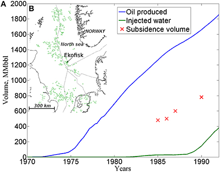
Figure 1. (A) Comparison of produced and injected volume with estimated subsidence volume during the production and (B) the map of Norwegian Sea with petroleum fields showing the location of Ekofisk field.

After the identification of the subsidence, a new production scheme started by waterflooding the reservoir and thus increasing the pore pressure and decreasing the effective stress inside the reservoir. However, the subsidence continued even after the new production scheme was introduced and pore pressure was raised to the initial values. Currently, the total subsidence observed since the beginning of oil production at the Ekofisk field is 9 m at the center of the field [8]. The high value of subsidence made it necessary to raise the platform and storage facilities above the subsiding bowl [9].

Several compaction models were created in an attempt to predict reservoir compaction and seafloor subsidence (e.g., [6, 10–12]). These apply a number of different phenomenological approaches to model the compaction of chalk based on macroscopic continuum equation models where parameters are fitted to experiments and observations. The first models explained the compaction as being elastic until the porous chalk riches a critical stress when sudden pore collapse happens resulting in a considerable plastic strain. Later models (e.g., [10]) included the idea that shear failure due to the build-up of differential stresses is responsible for the compaction. Inspired by these ideas several constitutive models for chalk were created most of which included 2–3 failure/yield mechanisms which they represented as separate failure surfaces intersecting each other. A generalized concept of the yield/failure surfaces is shown on Figure 2. With the introduction of water injection scheme the attention shifted toward the effect of water and how it decreases the material strength of chalk. This phenomenon is often referred as “water weakening” of chalk and several models were created to explain it (e.g., [14, 15]). A more detailed review of the previous models can be seen in Data Sheet 1 in Supplementary Material.

FIGURE 2

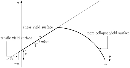
Figure 2. A generalization of the constitutive models yield surfaces in p-q stress invariant plane: tensile, shear failure, and pore collapse mechanism have their distinct yield surfaces, the resulting surface is a closed union of these surfaces. The tensile yield surface is characterized by p_t critical tensile strength, the shear surface by φ friction angle and c cohesion and the pore collapse surface by p_c critical stress and the shape of the ellipse. Some models introduce smooth changes close to the intersections while the model of Papamichos et al. [13] creates a similar shape yield surface by formulating their model as one mechanism.

Here we present a different approach, based on microscopic mechanisms with no fitting parameters using a universal creep model which combines microscopic fracturing and pressure solution where the local fracture stress is related to pore size, and then use a statistical mechanical approach to scale it up and predict strain rate at reservoir scale. We apply the model to field data and find that it reproduces the observed magnitude of seafloor subsidence. An advatage of this model over previous models is that it follows a bottom-up physics-based approach and therefore it provides a thorough insight into the underlying physical phenomena giving a higher predictive value.

2. The Ekofisk Reservoir

The Ekofisk field is an elongated anticlinal structure in the Southern part of the Norwegian North Sea with an aerial extent of about 6.8 by 9.3km. The thickness of the overlying sediments is 2840m in the central part of the field and increases toward the flanks [16]. Oil is produced from Ekofisk and the deeper Tor formation which are separated by a typically 15m thick low porosity chalk layer, the so-called Ekofisk Tight Zone. The thickness of the Ekofisk formation varies between 100 and 150m, while the thickness of the Tor formation varies between 75 and 150m.

The reservoir rocks are high-porosity fine-grade chalk, a limestone composed of coccolith fragments, the skeletal debris of unicellar algae (Coccolithophorids). The reservoir rock's porosity ranges between 30 and 48%, while the Ekofisk Tight Zone has porosity between 10 and 20%. Even the high porosity chalk has relatively low matrix permeability (i.e., the permeability of the matrix itself) between 1 and 5mD (1 – 5 · 10⁻¹⁵m²). Natural fractures give a high fracture permeability (i.e., the permeability caused by the macroscopic fractures) resulting in total chalk permeability between 10⁻¹³ and 10⁻¹⁴ m² (10 − 100mD) [16].

The overburden is mainly composed of clays and shales with thin interlayered limestone or silty layers [11, 14]. The permeability is extremely low (10⁻¹⁸ – 10⁻²¹ m², 10⁻³ – 10⁻⁶ mD) [16]. These rocks have a very low cohesional strength which makes them difficult to sample and therefore there is sparse and uncertain data about their rock properties [17].

In the early stage of oil production, pore fluid pressure dropped and the reservoir compacted, leading to a seafloor subsidence of up to 0.4 m per year which corresponds to a mean strain rate of 5 · 10⁻¹¹ $\frac{\text{m}}{\text{s}}$. Later a new reservoir management program was introduced maintaining pore pressure [18], however compaction and sea-floor subsidence continued.

3. Modeling the Subsidence

In this paper we predict subsidence history for the production phase before water injection using a very simple creep model (detailed in Keszthelyi et al. [19]). This model has the following simplifying assumptions:

• Prior to production, the reservoir rock is a non-reactive, elastic solid with a collection of pores with a probability distribution, p(r) of pore radii r.

• The reservoir rock is subject to confining stress σ of overlying sediments and a pore fluid pressure, P. All deformations are controlled by the effective stress σ_e = σ − P.

• When the effective stress exceeds a threshold, microscopic fractures will start to propagate from all pores with radius larger than a threshold value r_max. This threshold is defined by linear elastic fracture mechanics: $r_{max}=\gamma E∕{\sigma }_e^2$ where E is the Young's modulus of the rock and γ is the interfacial energy of the rock-pore fluid surface [20].

• The number of fractures created is proportional to the number of pores involved in the fracturing process. The fracture density ρ_f describes the abundance of the microscopic fractures and has the unit m∕s. We calculate this by statistical means from pore size distribution p(r) and initial porosity Φ₀.

• Fracturing is instantaneous and we neglect the strain in the solid due to the formation of these fractures and the poroelastic response of the rock.

• The new microscopic fractures are reactive sites where pressure solution takes place if there is water present. The fraction of water-wet fractures equals the water saturation S_w of the rock.

• The rate $\dot{\xi }$ of pressure solution at each reaction sites (expressed in m ∕ s) can be calculated by any pressure solution model independently from any other part of thee creep model. In this article we compared two approaches: a theoretical approach presented in Zhang et al. [21] and Pluymakers and Spiers [22] where pressure solution rate is a function of initial porosity Φ₀, temperature T and effective stress σ_e. In the other approach pressure solution rate is calculated from long-term strain rates measured in creep experiments.

The equations of the compaction model are presented in Data Sheet 1 in Supplementary Material.

The change in rock volume V = V_p + V_s, where V_s is the solid volume and V_p the pore volume, with time t, is expressed by the volumetric strain rate:

$\begin{array}{ll}{\dot{\epsilon }}_v(t)=\frac{1}{V}\frac{\partial V}{\partial t}=S_w·{\rho }_f\left({\sigma }_e,p(r)\right)\dot{\xi }\left({\sigma }_e,{\Phi }_0,T\right).& (1)\end{array}$

The input parameters of the creep model are: effective stress σ_e, initial porosity Φ₀, pore size distribution p(r), temperature T and water saturation S_w. Except for the effective stress we use constants obtained from literature (see Table 1). For pore size distribution p(r) we use a Weibull-type distribution with a shape parameter 1.5 and mean pore size of r_mean = 2.2μm as found in Japsen et al. [20]. Effective stress is calculated using the relation

$\begin{array}{ll}{\sigma }_e=\sigma -P.& (2)\end{array}$

TABLE 1

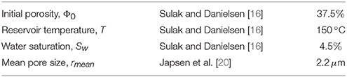
Table 1. Reservoir parameters used to calculate the subsidence history.

This is a much simpler definition for effective stress than used in some previous chalk compaction papers. In the following subsections we show that choosing this relation introduces only a small error in the result while the model is kept simple and physical. Then we present simple calculations to illustrate why the reservoir pressure P can be considered quasi equal to the pressure inside the boreholes. We then present a method used to calculate borehole pressures from production data and oil properties. Finally, we discuss how to calculate the other variable in the effective stress law: the confining stress σ.

3.1. Effective Stress Law

According to Coussy [23] effective stress definitions can be summerized in the following two equations assuming that deformations can be decomposed into a plastic and an elastic component:

$\begin{array}{ll}{\sigma }_{ij,e}^{\prime }={\sigma }_{ij}-\alpha P{\delta }_{ij}\text{ and }{\sigma }_{ij,p}^{\prime }={\sigma }_{ij}-{\beta }_{p}P{\delta }_{ij},& (3)\end{array}$

where ${\sigma }_{ij,e}^{\prime }$ denotes the element of the effective elastic stress tensor which is the driving stress for elastic strains, while ${\sigma }_{ij,p}^{\prime }$ is the element of the plastic stress tensor: the driving stress for plastic strains [23]. σ_ij is the element of the confining stress tensor, δ_ij is the Kronecker-delta function, P is the pore pressure, α is the Biot-coefficient and β_p is a plastic compressibility parameter.

The two constants (α and β_p) in the equations can vary between 0 and 1 and they describe how strain is distributed in the porous media between the solid matrix and the pore volume. α = 1 means an elastically incompressible matrix and 0 corresponds to the case when the pore volume is incompressible and all the elastic strains originate from the elastic deformation of the matrix. Similarly, β_p = 1 means a plastically incompressible matrix and 0 corresponds to an incompressible pore volume and all plastic stains originating from the plastic deformation of the matrix.

There have been several studies on the determination of the Biot-coefficient of chalk. While some of them claim a coefficient as low as 0.7–0.8 [24, 25], other experiments indicated a Biot-coefficient of 1 [26]. Hickman [5] showed considerably smaller bulk modulus (1–3 GPa) for chalk samples in the Ekofisk porosity range than the 70 GPa bulk modulus of calcite [27]. This implies a Biot-coefficient close to 1. Vajdova et al. [28] found experimentally that some plastic deformation (e.g., twinning) of calcite occurs in deforming limestones, however microcracking is the dominant deformation mechanism which implying a plastic compressibility parameter close to 1.

As the determination of the exact Biot-coefficient and compressibility parameter is beyond the scope of this article we assume that both are 1.

$\begin{array}{ll}\alpha =1\text{\hspace{1em}and\hspace{1em}}{\beta }_p=1& (4)\end{array}$

Furthermore, we assume that compaction is conrolled by the compressive stress:

$\begin{array}{ll}\sigma =\frac{1}{3}{\displaystyle \sum _i}{\sigma }_{ii}.& (5)\end{array}$

With these assumptions we can apply the simplified definition of the effective stress:

$\begin{array}{ll}{\sigma }_e(t):={\sigma }^{\prime }=\sigma -P(t).& (6)\end{array}$

3.2. Pressure Propagation

Oil is produced from the reservoir layer through boreholes penetrating the layer. Inside the boreholes they introduce a lower pressure than in the surrounding reservoir layer to facilitate the flow of pore fluids toward the well. To characterize the pressure changes inside the reservoir layer away from boreholes we treat the problem as the boreholes were uniformly distributed and calculate the fluid density function ρ(r, t) around a single well at a horizontal distance r from the borehole at time t after the pressure change inside the well took place.

The reservoir layer is treated as an axisymmetric layer with a finite thickness and with relatively high permeability compared to the surrounding (i.e., no fluid flow into or out from the layer). Its horizontal dimensions exceed the diameter of the reservoir field, the outer part is filled with water.

For the calculations we follow Muskat [29]'s approach based on the following two equations:

$\begin{array}{rcl}\mathrm{\text{Continuity equation}}& div(\Phi \rho \overrightarrow{v})=-\frac{\partial (\Phi \rho )}{\partial t}& (7)\end{array}$

$\begin{array}{rcl}\mathrm{\text{Darcy-law}}& \Phi \overrightarrow{v}=-\frac{k}{\mu }\nabla P& (8)\end{array}$

where Φ is the porosity, k is the permeability of the rock, μ is the dynamic viscosity of the fluid, ρ denotes the fluid density and $\overrightarrow{v}$ is the Darcy speed.

Furthermore, we assume that the reservoir fluid is compressible and it has the pressure-density relation ρ = ρ₀ · exp(βP) where β is the compressibility of the fluid and ρ₀ is a reference density at P = 0 pressure. By assuming that the initial fluid pressure was p₀ throughout the reservoir, and that there exists an outer boundary at distance r₂ where the fluid pressure remains constant and a borehole radius r_w inside which the pressure equals to well pressure p_w we obtain:

$\begin{array}{l}\rho (r,t)={\rho }_{stationary}+{\rho }_{scaling}·e^{-\kappa {\alpha }_n^{2}t}\\ \text{where}\kappa =\frac{\mu \Phi }{k}\left(\beta +\frac{1}{\Phi }\frac{\partial \Phi }{\partial P}\right)& (9)\end{array}$

and α_n is a constant depending on the boundary conditions. For details see Data Sheet 1 in Supplementary Material.

We perform calculations with material parameters relevant to the Ekofisk field (see Table 2) with a range of borehole radii r_w and reservoir outer boundary values r₂ (Figure 3) to estimate the half-time of the pressure propagation: the time required for that the amplitude of the pressure change become the half of the difference between the initial and the steady-state solution after pressure perturbation was introduces inside the borehole. We consider borehole radius r_w as unknown since this radius corresponds to an extremely highly fractured region around the physical borehole. Figure 3B shows that pressure propagation half times are in the order of minutes or hours in most of the cases. Therefore, we assume that the pressure respond instantaneously following the pressure changes in the boreholes.

TABLE 2

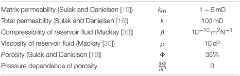
Table 2. Material and reservoir parameters (approximate values) for the estimation of pressure propagation characteristics.

FIGURE 3

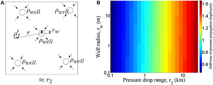
Figure 3. (A) Model of pressure propagation characteristic time calculations. We are interested in the pressure changes around a well: at any point with a distance r from the borehole. As fluid is moving toward the well pressure decreases in the reservoir. For the calculations our assumptions was that there exist a finite radius inside which pressure and thus fluid density (ρ_well) is constant—the well radius r_w—and an outer finite radius r₂ outside which pressure is constant and equals to the initial pressure. (B) Half-time of pressure propagation: the time necessary to experience 50% of pressure change—defined as the integral of the pressure change along the whole field—from the initial to the final pressure profile.

Based on this we calculated the pressure evolution during time from production data. The calculation assumes that the ratio between the produced gas and liquid phases at the surface depends on the gas and liquid fraction in the reservoir which is a function of the pressure inside the reservoir.

The stationary solution of the pressure propagation problem around a well is a conical pressure depression around the well where the center of the cone is the borehole where pressure is decreased. However, in the Ekofisk field hydrocarbons are produced from numerous wells penetrating into the reservoir and pressure is decreased in all of these wells. By 1980 forty wells were already producing from the reservoir. Given that the extent of the field is ~9 by 4 km, this implies that boreholes are placed closer than 1 km to each other. Hence the pressure depression cones are overlapping and the pressure changes inside the reservoir between two boreholes are small. Therefore, if we neglect the permeability inhomogeneites in the reservoir on the large scale we can assume a constant pressure throughout the reservoir as in [16, 17].

3.3. Calculating Reservoir Pressure from Production Data

To estimate how our model performs in terms of predicting the subsidence during the years of production, historical reservoir pressure data were needed. We use publicly available production and crude oil property data to make an estimae of the reservoir pressure history. We use the widely accepted concept of reservoir engineering (e.g., [31]) that the fraction of hydrocarbon in the liquid and gas state depends on the current pressure: at high pressure light components tend to dissolve in the liquid phase implying that above a certain threshold pressure (called bubble point) all hydrocarbons are in liquid phase.

Initially, when the reservoir was highly pressurized all hydrocarbons were in liquid phase. As pore pressure was decreased the reservoir became more saturated until it reached its bubble point (5990 psi, 41.3 MPa) in 1976 [1]. Thereafter two phases were present in the reservoir and the concentration of dissolved gas decreased while pressure declined. This resulted in a relative increase in the volume of gaseous phase both due to the liberation of natural gas from the liquid phase and to the relatively higher volume increase of the gaseous phase during decompression.

The increasing amount of gas inside the reservoir was clearly reflected in production data. Initially, before reaching the bubble point, the ratio of produced gas and oil—commonly referred as GOR, gas-oil-ratio—was constant and reflected the amount of gas deliberated from the fluid phase as the hydrocarbons were exposed to surface pressure. However, as pressure declined below the bubble point, gas bubbles appeared in the liquid phase and therefore the produced hydrocarbon contained considerably larger amount of gas which now were partly due to degassing from the liquid phase and partly due to the expansion of the gas bubbles originally present in the reservoir when they became exposed to surface conditions (see Figure 4).

FIGURE 4

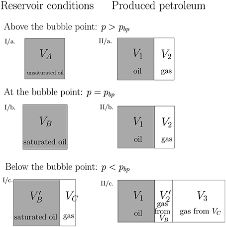
Figure 4. Volumes and phase changes of hydrocarbons inside the reservoir and during production as reservoir pressure is changed corresponding to same volume V₁ of oil produced at the surface. (I/a.) Initially there is a V_A volume unsaturated oil. (I/b.) As pressure is decreased to the bubble point oil becomes saturated and meanwhile there is a small expansion of its volume to V_B. (I/c.) As pressure is further decreased a free gas phase will form with V_C volume which largely depends on the reservoir pressure. Meanwhile the saturated oil phase also expands to $V_B^{\prime }$ volume. The right side of the figure shows the composition of the produced petroleum: all volumes are relative to the amount of oil produced and for simplicity it is V₁ in all cases. (II/a,b.) At the bubble point pressure and above it the gas phase with V₂ volume is formed by the degassing due to pressure drop from reservoir to surface conditions. Note that the gas-oil ratio is the same in both cases since the degasing starts only at the bubble point pressure. (II/c.) If pressure is decreased below the bubble point the produced gas is partly due to degasing ($V_2^{\prime }$) and partly to the free gas phase occupying a portion of the reservoir (V_C). $V_2^{\prime }$ is slightly smaller than V₂ since $V_B^{\prime }$ contains slightly less dissolved gas than V_B, however $V_3+V_2^{\prime }\gg V_2$. Note that the exact production volumes depend largely on reservoir pressure, larger reservoir pressures allow larger amount of petroleum to be produced, so in reality much less amount of oil is produced when pressure is lower. However, the dependence of produced petroleum to the reservoir pressure is controlled by the production technic, therefore, it is not show on this figure.

Knowing the amount of dissolved and free gas at different pressure and the relative volume of the phases at different pressure [32] it is possible to inversely calculate the pressure history from published GOR history data ([33], see Figure 5). We also account for the effect of injected gas volume assuming that due to the fact that reservoir fluid is already saturated it will mainly increase the free gas volume after compression. The calculated pressures can be seen on Figure 6.

FIGURE 5

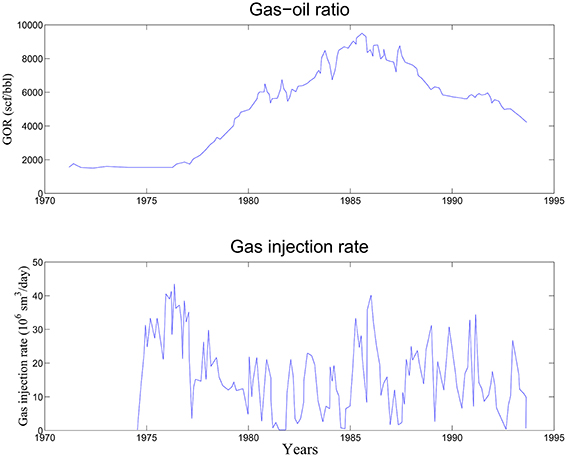
Figure 5. Gas injection rates and gas-oil ratio during the first period of production at the Ekofisk field. Source of data: Jakobsson et al. [33]. 1 ft³ ∕ barrel oil = 0.1781 sm³ ∕ sm³ oil. sm³: m³ at surface conditions.

FIGURE 6

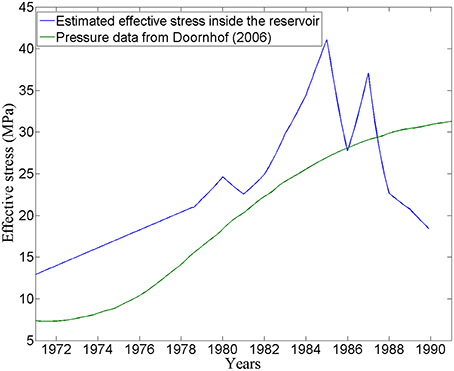
Figure 6. Estimated reservoir pressure during the years of production. The estimation was constrained by some data from Rhett [12] and Mes et al. [34]. Pressure history data presented in Doornhof et al. [35] are also plotted. SI units are used, 1 MPa = 145 psi.

3.4. Overburden Behavior

A schematic view of the Ekofisk reservoir during production can be seen in Figure 7. The majority of reservoir scale simulations treat overburden as a linear elastic material which is fully coupled to the reservoir and therefore follows its subsidence.

FIGURE 7

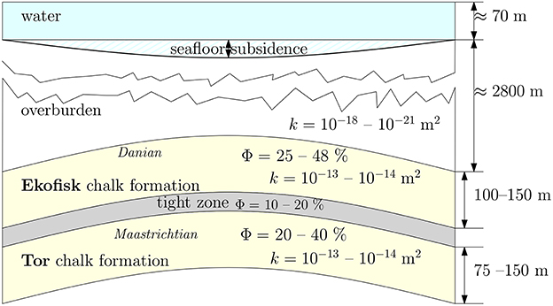
Figure 7. Schematic view of the produced Ekofisk field showing the layering of the chalk reservoir, the thick overburden, and the shallow layer of seawater. The most important material parameters (k: permeability and Φ porosity) are shown on the figure. SI units are used, 9.87 · 10⁻¹⁰ m² = 1 mD.

However, it has been pointed out that the overburden has a certain rigidity compared to the reservoir [7, 16]. Hamilton et al. [36] suggested that fractures formed inside the overburden as a consequence of stress field change and they supported the idea with the argument that the overburden has a high smectite content which facilitate fracturing.

The existence and nature of fractures inside the overburden are not yet completely understood. Observations show that casing deformations inside the overburden are most pronounced inside those wells which have a horizontal position between the central and the peripheral part of the reservoir [17, 37]. This implies that a fracture network is present inside the overburden and the location of the fractures coincide with the sites where stress is maximal due to arching effect. To better understand the overburden behavior future work is necessary.

For simplicity, we assume that the overburden is completely soft and follows the motion of the compacting reservoir layer and we neglect the effect of shear. Therefore, the subsidence rate, ṡ(t) of the field can be estimated as the product of the strain rate ${\dot{\epsilon }}_v$ corresponding to the reservoir pressure P(t) and the thickness of the reservoir h:

$\begin{array}{ll}ṡ(t)={\dot{\epsilon }}_v\left(P(t)\right)·h.& (10)\end{array}$

4. Results

The model of Keszthelyi et al. [19] can be used to predict compaction and subsidence if the pore size distribution and the average porosity is known. However, the pore size distribution is somewhat uncertain. In the following we assume a Weibull distribution ([38], see subfigure in Figure 8) with 2.2μm as mean pore size [20] that was fitted to SEM image data of chalk from wells in the same formation. We calculate microscopic fracture density as a function of effective stress (see Figure 8) with these input parameters. It can be seen that at lower effective stresses the fracture density is virtually zero. It rises very rapidly in a very narrow effective stress range and it flattens out at higher effective stress to an asymptotic value around 10⁵m⁻¹.

FIGURE 8

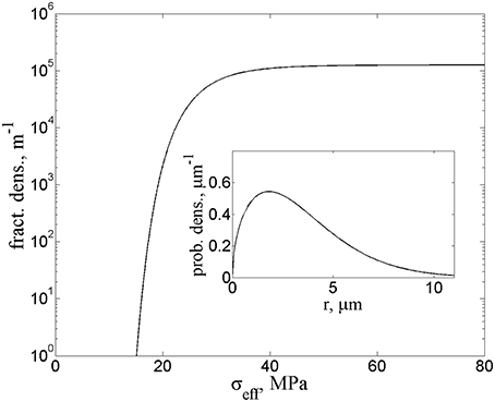
Figure 8. Fracture density as function of effective stress if Weibull-type distribution and 2.2μm average pore diameter is assumed. The pore size distribution's density function is shown in the inset. It is defined by the equation $p(r)=1.5{\lambda }^{-1}\sqrt{r∕\lambda }·e^{-{(r∕\lambda )}^{1.5}}$ where the shape factor λ = 1.5. SI units are used, 1 MPa = 145 psi.

Due to the uncertainty of the pore size distribution data we calculate fracture densities for a range of mean pore sizes relevant to the Ekofisk field, while preserving the shape of the pore size distribution. We plotted the fracture density as a function of two variables: effective stress σ_e and mean pore size r_mean (see Figure 9). It can be seen that fracture density varies in a relatively narrow band of effective stress values, however, the interval where this band is exactly located is a non-linear function of the mean pore size: for smaller pores only larger stress produce fracturing, while for larger pores require smaller stresses can produce fracturing.

FIGURE 9

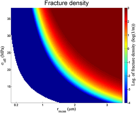
Figure 9. Fracture density as a function of effective stress and mean pore diameter assuming a Weibull distribution (similar to Figure 8). The figure is color-coded representing the magnitude—logarithm—of the fracture density. SI units are used, 1 MPa = 145 psi.

We also calculate the resulting strain rate in the same range of the variables by using both approaches for the pressure solution rate calculation (theoretical model: Figure 10 and long-term model: Figure 11). Initial (pre-production) and maximal effective stress values are marked with horizontal lines and strain rates corresponding to the initial and maximal effective stress using 2.2μm mean pore size value are also marked. An isoline at a strain rate of 10⁻¹¹s⁻¹ corresponding to the average measured strain rate is also shown. In the theoretical model the dissolution rate depends on effective stress while in the long-term model dissolution rate remains constant and fracture density has the only pressure dependence.

FIGURE 10

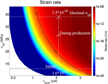
Figure 10. Strain rate calculated assuming a Weibull distribution of pore size, using a range of mean pore size and effective stress values and dissolution rates calculated from the theoretical model. A line representing the modeled mean pore size for Ekofisk chalk (following Japsen et al. [20]) and average strain rate for this period is also plotted on the figure. The contour line crosses the line corresponding to Ekofisk chalk. SI units are used, 1 MPa = 145 psi.

FIGURE 11

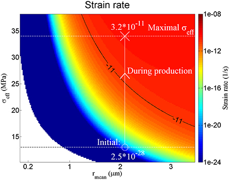
Figure 11. Long-term strain rate calculated assuming a Weibull distribution of pore size, using a range of mean pore size and effective stress values and dissolution rates calculated from the long-term strain rates of Zhang et al. [21] experiments. A line representing the modeled mean pore size for Ekofisk chalk (following Japsen et al. [20]) and average strain rate for this period is also plotted on the figure. The contour line crosses the line corresponding to Ekofisk chalk. SI units are used, 1 MPa = 145 psi.

In both cases, the initial effective stress corresponds to a negligible amount of compaction, while at maximum effective values we get realistic predicted strain rates, the average measured strain rate is between the initial and maximal values.

In order to compare model prediction with field data we calculate the subsidence rate and resulting subsidence for a 20 year long period (see Figures 12, 13) using the estimated pressure history data calculated from the produced amount of hydrocarbons (see Figure 6 and Section 3.3 for the principles of the calculation) and estimated pressure history curve from Doornhof et al. [35]. These calculations show that the theoretical model gives subsidence comparable to field observations, and by using the estimates from production curves the model prediction agrees very well with field observations, while the model based on the long-term compaction experiments somewhat underestimates the compaction, though it gives significantly better estimates than the poroelastic model of Segall [4].

FIGURE 12

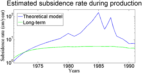
Figure 12. Estimated subsidence rate according to the model using reservoir pressure history estimations (see Section 3.3). The resulting subsidence rate are similar to the observed rates.

FIGURE 13

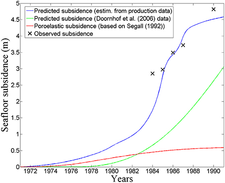
Figure 13. Estimated subsidence during the first period of the production. Estimation based on pressure history calculations in Section 3.3 and on data from Doornhof et al. [35]. Predictions of the poroelastic model of Segall [4] is also plotted.

5. Concluding Remarks

We were able to apply a micromechanical model of carbonate compaction which combines microscopic fracturing (pore failure) with creep (pressure solution) using upscaling to reservoir scale through the concept of fracture density. This model predicted surprisingly well the observed compaction and subsidence making it the first microstructural model which can explain the Ekofisk subsidence. The model contains a very small number of internal parameters: Young's modulus of chalk, the water-wet interfacial energy of calcite and reaction constants describing the dissolution-precipitation kinetics and diffusion of calcite all of which can be meausured with simple physical experiments independently. The input parameters are pore size distribution, water saturation, porosity and pressure history. Furthermore, the model is based on physical assumptions, eliminating the need of unphysical fitting parameters. We believe this results in a higher predictive power than previously used models with a large number of fine-tuned parameters.

The discrepancy between the model prediction and field observations is due to the uncertainty of input parameters and the simplifying assumptions during the application or inside the model.

The model is very sensitive to the pore size distribution. Application of this model depends on reliable data for the actual situation to estimate the pore size distribution. Pore size distribution data can be obtained by accurate measurements: currently the most accurate being X-ray microtomography data, although only a few measurements exist currently. Mercury injection data are considerably more common and can be used as a less reliable source of pore size distribution measurements since it does not measure pore size distribution directly but pore throat distribution.

A previous study [20] found that the Weibull distribution fit observations reasonably well for chalk samples from wells close to the Ekofisk field. There have been several other measurements on chalks from different origin: Hellmann et al. [39] measured pore size distribution by mercury-injection on chalk samples from Paris basin and found a sigmoid-type cummulative pore size distribution with some larger pores in addition. Price et al. [40] investigated chalk samples from the Upper Chalk formation and found also a sigmoid-type cummulative pore size distribution function, however the mean pore size differs from that of Japsen et al. [20]. Being the closest analogue to the Ekofisk field we used Weibull distribution presented in Japsen et al. [20].

Investigating the effect of water saturation can presumably help to address the question of ongoing subsidence during production with water injection when the pore pressure was increased to the original values. As water is pumped in and water saturation increases inside the reservoir the newly entering water can also flow into the initially oil-filled recent microscopic fractures triggering pressure solution there. This may cause the reservoir to compact after the start of injection, but to settle down as water saturation levels to equilibrium. The model also shows that there is a large potential of further subsidence if water saturations increase in the reservoir and thus it can serve as an explanation for “water weakening” effect of chalk.

Inhomogeneities inside the reservoir are present in every scale. Apart from the variability of material parameters (porosity, pore size distribution, and water saturation) a complicated network of macroscopic fractures makes the modeling difficult. While some part of the reservoir are extensively fractured and pressure changes can happen rapidly, other parts of the reservoir contain less macroscopic fractures slowing down pressure propagation and the whole compaction process. In order to characterize the compaction and subsidence in detail these variations should be considered.

The current micromechanical model keeps the model of the microscopic fracturing process simple and claims that compaction is mainly driven by vertical stress. This approach neglects the modifying effect of horizontal stresses which are present as far-field tectonic stresses, while laterial variations in the compaction process due to different reservoir parameters can also cause local build-up of horizontal stresses. Therefore, a 3-dimensional reservoir-scale model of compaction should take into account the effect of horizontal stresses and should be tested against a detailed data on the compaction process.

Author Contributions

All authors listed, have made substantial, direct and intellectual contribution to the work, and approved it for publication.

Conflict of Interest Statement

The authors declare that the research was conducted in the absence of any commercial or financial relationships that could be construed as a potential conflict of interest.

Acknowledgments

We gratefully acknowledge the support of the FlowTrans Marie-Curie ITN for the funding of the PhD grant of DK (under grant agreement no. 31688 in the European Seventh Framework Programme). Thanks to Anja Røyne and Amélie Neuville for their valuable comments and for the employees of ConocoPhilips Norway for the thoughtful discussions.

Supplementary Material

The Supplementary Material for this article can be found online at: https://www.frontiersin.org/article/10.3389/fphy.2016.00004

References

1. Hermansen H, Landa G, Sylte J, Thomas L. Experiences after 10 years of waterflooding the Ekofisk Field, Norway. J Petrol Sci Eng. (2000) 26:11–8. doi: 10.1016/S0920-4105(00)00016-4

CrossRef Full Text | Google Scholar

2. Boade R, Chin L, Siemers W. Forecasting of Ekofisk reservoir compaction and subsidence by numerical simulation. J Petrol Technol. (1989) 41:723–8. doi: 10.2118/17855-PA

CrossRef Full Text

3. Geertsma J. Land subsidence above compacting oil and gas reservoirs. J Petrol Technol. (1973) 25:734–44. doi: 10.2118/3730-PA

CrossRef Full Text | Google Scholar

4. Segall P. Induced stresses due to fluid extraction from axisymmetric reservoirs. Pure Appl Geophys. (1992) 139:535–60.

Google Scholar

5. Hickman RJ. Formulation and Implementation of a Constitutive Model for Soft Rock. Ph.D. dissertation, Virginia Polytechnic Institute and State University (2004).

6. Johnson J, Rhett D. Compaction behavior of Ekofisk chalk as a function of stress. In: European Petroleum Conference. London (1986). doi: 10.2118/15872-MS

CrossRef Full Text

7. Sulak R, Thomas L, Boade R. 3D reservoir simulation of ekofisk compaction drive (includes associated papers 24317 and 24400). J Petrol Technol. (1991) 43:1272–8.

Google Scholar

8. Jones G, Kendall JM, Bastow I, Raymer D, Wuestefeld A. Characterization of fractures and faults: a multi-component passive microseismic study from the Ekofisk reservoir. Geophys Prospect. (2014) 62:779–96. doi: 10.1111/1365-2478.12139

CrossRef Full Text | Google Scholar

9. Gutierrez M. Fully coupled analysis of reservoir compaction and subsidence. In: European Petroleum Conference. London (1994). doi: 10.2118/28900-MS

CrossRef Full Text

10. Chin L, Boade R, Prevost J, Landa G. Numerical simulation of shear-induced compaction in the Ekofisk reservoir. Int J Rock Mech Mining Sci Geomech Abstr. (1993) 30:1193–200.

Google Scholar

11. Abdulraheem A, Zaman M, Roegiers JC. A finite-element model for Ekofisk field subsidence. J Petrol Sci Eng. (1994). 10:299–310.

Google Scholar

12. Rhett DW. Ekofisk revisited: a new model of Ekofisk reservoir geomechanical behavior. In: EUROCK 98 Symposium. Trondheim (1998). doi: 10.2118/47273-MS

CrossRef Full Text

13. Papamichos E, Brignoli M, Santarelli F. An experimental and theoretical study of a partially saturated collapsible rock. Mech Cohesive-frictional Mater. (1997) 2:251–78.

Google Scholar

14. Plischke B. Finite element analysis of compaction and subsidence-Experience gained from several chalk fields. Rock Mech Petrol Eng. Delft (1994). doi: 10.2118/28129-MS

CrossRef Full Text

15. Datcheva M, Charlier R, Collin F. Constitutive equations and numerical modelling of time effects in soft porous rocks. In: Numerical Analysis and Its Applications. Berlin; Heidelberg: Springer (2001). pp. 222–29.

16. Sulak R, Danielsen J. Reservoir aspects of Ekofisk subsidence. J Petrol Technol. (1989) 41:709–16.

Google Scholar

17. Chin L, Boade R, Nagel B, Landa G. Numerical simulation of Ekofisk reservoir compaction and subsidence: treating the mechanical behavior of the overburden and reservoir. Rock Mech Petrol Eng. Delft (1994). doi: 10.2118/28128-MS

CrossRef Full Text

18. Sylte J, Thomas L, Rhett D, Bruning D, Nagel N. Water induced compaction in the Ekofisk field. In: SPE Annual Technical Conference and Exhibition. Houston, TX (1999). doi: 10.2118/56426-MS

CrossRef Full Text

19. Keszthelyi D, Dysthe DK, Jamtveit B. Modeling of carbonate compaction by pore failure and pressure solution. J Geophys Res. (in review).

20. Japsen P, Dysthe D, Hartz E, Stipp SLS, Yarushina V, Jamtveit B. A compaction front in North Sea chalk. J Geophys Res. (2011) 116:B11208. doi: 10.1029/2011JB008564

CrossRef Full Text | Google Scholar

21. Zhang X, Spiers CJ, Peach CJ. Compaction creep of wet granular calcite by pressure solution at 28 C to 150 C. J Geophys Res. (2010) 115:B09217. doi: 10.1029/2008JB005853

CrossRef Full Text | Google Scholar

22. Pluymakers A, Spiers C. Compaction creep of simulated anhydrite fault gouge by pressure solution: theory v. experiments and implications for fault sealing. Geol Soc Lond Spec Publ. (2014) 409:SP409–6. doi: 10.1144/SP409.6

CrossRef Full Text | Google Scholar

23. Coussy O. Poromechanics. Chichester: John Wiley & Sons (2004).

Google Scholar

24. Alam MM, Fabricius IL, Christensen HF. Static and dynamic effective stress coefficient of chalk. Geophysics (2012) 77:L1–11. doi: 10.1190/geo2010-0414.1

CrossRef Full Text | Google Scholar

25. Kristiansen TG, Plischke B. History matched full field geomechanics model of the Valhall Field including water weakening and re-pressurisation. In: SPE EUROPEC/EAGE Annual Conference and Exhibition. Barcelona: Society of Petroleum Engineers (2010). doi: 10.2118/131505-MS

CrossRef Full Text

26. Warpinski N, Teufel L. Determination of the effective stress law for permeability and deformation in low-permeability rocks. SPE Form Eval. (1992) 7:123–31.

Google Scholar

27. Dvorkin J, Prasad M, Sakai A, Lavoie D. Elasticity of marine sediments: rock physics modeling. Geophys Res Lett. (1999) 26:1781–4.

Google Scholar

28. Vajdova V, Baud P, Wu L, Wong Tf. Micromechanics of inelastic compaction in two allochemical limestones. J Struct Geol. (2012) 43:100–17. doi: 10.1016/j.jsg.2012.07.006

CrossRef Full Text

29. Muskat M. The Flow of Homogeneous Fluids through Porous Media, Vol. 12. New York, NY: McGraw-Hill (1937).

30. Mackay D. Ekofisk Crude Oil Properties. Version 4, October 2007 to April 2008, Gatineau, QC: Environment Canada, Emergencies Science and Technology Division (1995).

31. Dake LP. Fundamentals of Reservoir Engineering. Amsterdam: Elsevier (1983).

Google Scholar

32. NPD. Norwegian Petroleum Directorate Technical Report: Reservoir Fluid Study for Phillips Petroleum Company - Norway, 2/4-2X well DST No. 6B Ekofisk field, North Sea, Norway (1970). Available online at: http://www.npd.no/engelsk/cwi/pbl/wellbore_documents/97_05_2_4_3(2X)_Reservoir_Fluid_Study_DST_6.pdf

33. Jakobsson NM, Christian TM. Historical performance of gas injection of Ekofisk. In: SPE Annual Technical Conference and Exhibition. New Orleans, LA: Society of Petroleum Engineers (1994). doi: 10.2118/28933-MS

CrossRef Full Text | Google Scholar

34. Mes MJ. Ekofisk reservoir pressure drops and seabed subsidence. In: Offshore Technology Conference. Houston, TX: Offshore Technology Conference (1990). doi: 10.4043/6241-MS

CrossRef Full Text | Google Scholar

35. Doornhof D, Kristiansen TG, Nagel NB, Pattillo PD, Sayers C. Compaction and subsidence. Oilfield Rev. (2006) 18:50–68.

Google Scholar

36. Hamilton JM, Mailer AV, Prins MD. Subsidence-induced shear failures above oil and gas reservoirs. In: The 33th US Symposium on Rock Mechanics (USRMS). Santa Fe, NM: American Rock Mechanics Association (1992).

37. Schwall G, Denney C. Subsidence induced casing deformation mechanisms in the Ekofisk field. Rock Mech Petrol Eng. Delft (1994). doi: 10.2118/28091-MS

CrossRef Full Text | Google Scholar

38. Weibull, W. A statistical distribution function of wide applicability. J. Appl. Mech. (1951). 18:293–297.

39. Hellmann R, Renders PJ, Gratier JP, Guiguet R. Experimental pressure solution compaction of chalk in aqueous solutions. Part 1. Deformation behavior and chemistry. In: Hellmann R and Wood SA, editors. Water-Rock Interaction, Ore Deposits, and Environmental Geochemisty: A tribute to David A Crerar, Vol. 7, (Washington, DC: Geochemical Society) (2002). pp. 129–52.

40. Price M, Bird M, Foster S. Chalk pore-size measurements and their significance. Water Serv. (1976) 80:596–600.

41. Johnson J, Rhett D, Siemers W. Rock mechanics of the Ekofisk reservoir in the evaluation of subsidence. In: Offshore Technology Conference. Houston, TX (1988). doi: 10.4043/5621-MS

CrossRef Full Text

42. Shao J, Henry J. Development of an elastoplastic model for porous rock. Int J Plast. (1991) 7:1–13.

Google Scholar

43. Andersen M, Foged N, Pedersen H. The rate-type compaction of a weak North Sea chalk. In: The 33th US Symposium on Rock Mechanics (USRMS). Santa Fe, NM: American Rock Mechanics Association (1992).

44. Andersen M, Foged N, Pedersen H. The link between waterflood-induced compaction and rate-sensitive behavior in a weak North Sea chalk. In: Proceedings of 4th North Sea Chalk Symposium. Deauville (1992).

45. Nagel N. Compaction and subsidence issues within the petroleum industry: from Wilmington to Ekofisk and beyond. Phys Chem Earth A Solid Earth Geod. (2001) 26:3–14. doi: 10.1016/S1464-1895(01)00015-1

CrossRef Full Text | Google Scholar

46. Du J, Olson JE. A poroelastic reservoir model for predicting subsidence and mapping subsurface pressure fronts. J Petrol Sci Eng. (2001) 30:181–197. doi: 10.1016/S0920-4105(01)00131-0

CrossRef Full Text | Google Scholar

47. De Gennaro V, Delage P, Cui YJ, Schroeder C, Collin F. Time-dependent behaviour of oil reservoir chalk: a multiphase approach. Soils Found. (2003) 43:131–47. doi: 10.3208/sandf.43.4_131

CrossRef Full Text | Google Scholar

48. Collin F, Cui YJ, Schroeder C, Charlier R. Mechanical behaviour of Lixhe chalk partly saturated by oil and water: experiment and modelling. Int J Numerical Anal Methods Geomech. (2002) 26:897–924. doi: 10.1002/nag.229

CrossRef Full Text | Google Scholar