A Matrix Model from String Field Theory

1. Introduction

Two different candidates for the nonperturbative formulation of string theory have been known—string field theory (SFT) and matrix model. It is commonly believed that they are just different descriptions of the underlying theory. Therefore, it is important to investigate the relationship between these formulations. However, a few examples have been known to reduce open SFT (OSFT) [1] to certain matrix models. First is OSFT for topological A or B model [2] which reduces to Chern-Simons matrix model [3] or ordinary Hermitian matrix model [4] respectively. Second is OSFT for (2,1) minimal string [5] which reduces to Kontsevich matrix model [6]. In addition, less direct examples for c = 1 [7], c = 0 [8], and critical [9] strings have been known. In those examples, each matrix model is obtained from different OSFT associated with particular boundary conformal field theory (BCFT). A systematic way to derive different matrix models from OSFT in fixed background has not yet known. Finding such method is important to study the background independence of OSFT.

In this paper, we present an example for such method. Our idea is simple: instead of varying BCFT, we start with a general setup in critical string, and approximate the string field to its first few components. An example we will study is the level truncation in the universal sector [10] of critical (D = 26) OSFT in which the string field is approximated at level n as

$\begin{array}{ll}\text{Ψ}={\psi }_0+{\psi }_1+{\psi }_2+\cdots +{\psi }_n.& (1)\end{array}$

 ¹

Given this approximation, the OSFT action [1] immediately reduces to a matrix action²

$\begin{array}{ll}S=a_{mn}Tr\left[M_m{M}_n\right]+b_{mnp}Tr\left[M_m{M}_n{M}_p\right],& (2)\end{array}$

where M_n is a Hermitian matrix. The approximation is known to work well in the first few level and improves quickly as the level increases [11–15].

A possible reason that such method has not yet been examined is the lack of understanding of Chan-Paton factors in OSFT. Although Chan-Paton factors can be introduced to OSFT consistently, their origin has not yet been explained. Recently, Erler and Maccaferri proposed a new construction of classical solutions of OSFT in terms of the regularized boundary conditions changing (BCC) projectors [16]. Their construction covers a wide range of backgrounds including multiple D-branes, which is the main interest of present paper. Following their work, Kishimoto, Masuda, Takahashi, and Takemoto (KMTT) demonstrated that N Chan-Paton factors naturally arise from the decomposition of string field in terms of the regularized BCC projectors [17]. SFT expanded around the multiple D-branes solution was interpreted as a system of N + 1 D-branes. We will employ their formulation as our foundation.

This paper is organized as follows. Section 2 introduces KMTT formulation. In Section 3, we derive a one-matrix model in terms of the level truncation. In Section 4, we derive the partition function of the model both in finite and large N. Section 5 summarizes our results and further discussions are given.

2. KMTT Formulation

Let us briefly review the KMTT formulation [17] of OSFT. They begin with Erler-Maccaferri solution for multiple D-branes [16]

$\begin{array}{ll}{\text{Ψ}}_0={\text{Ψ}}_T-{\displaystyle \sum _{a=1}^N}{\Sigma }_a{\text{Ψ}}_T{\overline{\Sigma }}_a,& (3)\end{array}$

where Ψ_T is the tachyon vacuum solution and Σ_a and ${\overline{\Sigma }}_a$ are the regularized BCC projectors which obey

$\begin{array}{ll}{\overline{\Sigma }}_a{\Sigma }_b={\delta }_{ab},Q_T{\Sigma }_a=Q_T{\overline{\Sigma }}_a=0.& (4)\end{array}$

Here Q_T is the kinetic operator at the tachyon vacuum defined by

$\begin{array}{ll}{Q}_T\text{Ψ}=Q_B\text{Ψ}+{\text{Ψ}}_T\text{Ψ}+\text{Ψ}{\text{Ψ}}_T.& (5)\end{array}$

The index a in Σ_a or ${\overline{\Sigma }}_a$ is a Chan-Paton factor which labels D-branes. The solution (Equation 3) carries degrees of freedom required for multiple D-branes. We further expect that non-Abelian gauge gauge symmetry is realized in OSFT expanded around (Equation 3). KMTT [17] introduced the decomposition of the string field which realizes this:

$\begin{array}{ll}\text{Ψ}=\chi +{\chi }_a{\overline{\Sigma }}_a+{\Sigma }_a{\overline{\chi }}_a+{\overline{\Sigma }}_a{\varphi }_{ab}{\Sigma }_b,& (6)\end{array}$

where χ, χ_a, ${\overline{\chi }}_a$ and χ_ab are component string fields. By expanding OSFT action around Ψ₀ according to Equation (6), they derived the matrix action

$\begin{array}{ll}S=S_1+S_2+S_3,& (7)\end{array}$

$\begin{array}{ll}{S}_1=-\frac{1}{g^2}Tr{\displaystyle \int }\left(\frac{1}{2}\varphi Q_B\varphi +\frac{1}{3}{\varphi }^3\right),& (8)\end{array}$

$\begin{array}{ll}{S}_2=-\frac{1}{g^2}{\displaystyle \int }\left(\frac{1}{2}\chi Q_T\chi +\frac{1}{3}{\chi }^3\right),& (9)\end{array}$

$\begin{array}{ll}{S}_3=-\frac{1}{g^2}{\displaystyle \int }\left(\frac{1}{2}{\overline{\chi }}_a{Q}_{T0}{\chi }_a+{\overline{\chi }}_a\chi {\chi }_a+{\overline{\chi }}_a{\varphi }_{ab}{\chi }_b\right),& (10)\end{array}$

where Q_T0 is the kinetic operator defined by Q_T0Ψ = Q_BΨ + Ψ_TΨ. The trace in (Equation 8) runs over indices of ϕ_ab, and identical indices in Equation (10) are to be summed over³. KMTT [17] claimed that (Equation 7) describes N + 1 D-branes rather than N D-branes. In addition to the N unstable D-branes, there is a “D-brane” at the tachyon vacuum described by χ. According to their interpretation, ϕ_ab connects two unstable D-branes a and b while χ_a connects D-brane a with the D-brane at the tachyon vacuum. χ represents fluctuation on the D-brane at the tachyon vacuum.

A remarkable feature of the action (Equation 7) is the presence of the “vector” sector described by χ_a and ${\overline{\chi }}_a$, which has not been found in literature. The action S₃ is quadratic for the vectors therefore can be integrated out in the path integral. With assuming suitable gauge fixing, we perform path integral for χ_a and ${\overline{\chi }}_a$ and obtain a determinant factor

$\begin{array}{ll}det{(Q_{T0}+\varphi +\chi )}^{-1}& (11)\end{array}$

in the partition function. In the following sections, we will evaluate this determinant by truncating the string field rather than imposing conventional gauge condition such as linear gauge [18].

3. Truncation to Matrices

Although the string fields presented in previous section carry Chan-Paton factors, they also depend on infinitely many labels which distinguish each state in a BCFT. In order to make our analysis tractable, we introduce an approximation in which dynamical variables reduce to matrices. Let us consider the string field in the universal sector⁴ truncated at level n, where the level is defined by eigenvalue of the kinetic operator of OSFT. Denoting the level k base element of the string field ψ_k, we truncate each component in Equation (6) as

$\begin{array}{l}{\varphi }_{ab}={\displaystyle \sum _{k=1}^n}{M}_{ab}^{(k)}{\psi }_k,{\chi }_a={\displaystyle \sum _{k=1}^n}{\xi }_a^{(k)}{\psi }_k,{\overline{\chi }}_a={\displaystyle \sum _{k=1}^n}{\overline{\xi }}_a^{(k)}{\psi }_k,\\ \chi ={\displaystyle \sum _{k=1}^n}{t}^{(k)}{\psi }_k,& (12)\end{array}$

where $M_{ab}^{(k)}$ is a Hermite matrix, ${\xi }_a^{(k)}$ is a complex vector, ${\overline{\xi }}_a^{(k)}$ is its complex conjugate, and t^(k) is a real number. Note that these component fields do not depend on any other variables. As a concrete example of such truncation, we choose the expansion examined in Zeze [19] for dressed ${B}$₀ gauge [20]. In this case, the level k base is given by

$\begin{array}{ll}{\psi }_k=c{K}^{n}Bc\frac{1}{1+K},& (13)\end{array}$

where K, B, c are the elements of the KBc algebra [21]. We would like to study level 1 truncation in which string fields are given by

$\begin{array}{llll}\hfill {\varphi }_{ab}& =M_{ab}^{(0)}{\psi }_0+M_{ab}^{(1)}{\psi }_1,& & (14)\end{array}$

$\begin{array}{llll}\hfill {\chi }_a& ={\xi }_a^{(0)}{\psi }_0+{\xi }_a^{(1)}{\psi }_1,& & (15)\end{array}$

$\begin{array}{llll}\hfill {\overline{\chi }}_a& ={\overline{\xi }}_a^{(0)}{\psi }_0+{\overline{\xi }}_a^{(1)}{\psi }_1,& & (16)\end{array}$

$\begin{array}{llll}\hfill \chi & =t^{(0)}{\psi }_0+t^{(1)}{\psi }_1.& & (17)\end{array}$

A matrix action obtained by this truncation is rather complex since it includes both level 0 and 1 fields. However, it is possible to reduce degrees of freedom further. It is know that level 1 fields cannot have cubic terms since [19]

$\begin{array}{ll}{\displaystyle \int }{\psi }_1^3=0.& (18)\end{array}$

Thus, level 1 fields are quadratic in the action and can be integrated out using equations of motion. With the help of the explicit values of products of the basis ψ₀ and ψ₁ evaluated in Zeze [19], a nontrivial solution of equations of motion for $M_{ab}^{(1)},{\xi }_a^{(1)},{\overline{\xi }}_a^{(1)}$, and t⁽¹⁾ turns out to be

$\begin{array}{ll}{M}_{ab}^{(0)}=M_{ab}^{(1)},{\xi }_a^{(0)}={\xi }_a^{(1)},{\overline{\xi }}_a^{(0)}={\overline{\xi }}_a^{(1)},t^{(0)}=t^{(1)}.& (19)\end{array}$

By this assignment, four string fields in Equation (12) become proportional to Erler-Schnabl solution [20]:

$\begin{array}{ll}{\text{Ψ}}_T=c(1+K)Bc\frac{1}{1+K}.& (20)\end{array}$

Thus, the four fields⁵ can be written as

$\begin{array}{ll}{\varphi }_{ab}=M_{ab}{\text{Ψ}}_T,{\chi }_a={\xi }_a{\text{Ψ}}_T,{\overline{\chi }}_a={\overline{\xi }}_a{\text{Ψ}}_T,\chi =t{\text{Ψ}}_T.& (21)\end{array}$

Although only few fields are included in the approximation, we expect that it well captures the essence of the dynamics of D-branes, as is the case in the conventional level truncation analysis. An evidence that supports our expectation is that the truncation interpolates between two analytic solutions: one is the Erler-Maccaferri's multiple D-branes denoted as $(M_{ab},{\xi }_a,{\overline{\xi }}_a,t)=(0,0,0,0)$ while the other is the perturbative vacuum, also denoted as (δ_ab, 0, 0, −1).

Let us derive the truncated action. The requirement that Ψ_T reproduces the correct value of the D-brane tension is represented by

$\begin{array}{l}{\displaystyle \int }{\text{Ψ}}_T{Q}_B{\text{Ψ}}_T=-\frac{3}{{\pi }^2},{\displaystyle \int }{\text{Ψ}}_T{Q}_{T0}{\text{Ψ}}_T=0,\\ {\displaystyle \int }{\text{Ψ}}_T{Q}_T{\text{Ψ}}_T=+\frac{3}{{\pi }^2},{\displaystyle \int }{\text{Ψ}}_T^3=+\frac{3}{{\pi }^2}.& (22)\end{array}$

Applying these to Equation (7), we find

$\begin{array}{l}S=-\frac{1}{{g^{\prime }}^2}[\text{Tr}\left(-\frac{1}{2}{M}^2+\frac{1}{3}{M}^3\right)+\frac{1}{2}{t}^2+\frac{1}{3}{t}^3\\ +{\overline{\xi }}_a(t{\delta }_{ab}+M_{ab}){\xi }_b]\text{},& (23)\end{array}$

where we have rescaled the open string coupling as

$\begin{array}{ll}\frac{1}{g^{\prime 2}}=\frac{3}{g^2{\pi }^2}.& (24)\end{array}$

For later convenience, we shift M to M + 1 and omit the prime in g′. Then, ignoring constant shift, we obtain an action

$\begin{array}{ll}S=-\frac{1}{g^2}\left[TrW(M)+W(t)+\overline{\xi }(1+t+M)\xi \right],& (25)\end{array}$

where $W(x)=\frac{1}{2}{x}^2+\frac{1}{3}{x}^3$. In this way, the truncation (Equation 12) reduces OSFT action to a cubic matrix action coupled with a scalar and complex vectors⁶. The partition function for Equation (25) can be obtained by employing the standard technique of matrix model⁷. As readily found in Equation (25), the action is invariant under U(N) transformation $M\to UM{U}^{†},\xi \to U\xi ,\overline{\xi }\to \overline{\xi }{U}^{†}$, where U denotes an U(N) matrix. This is a residual gauge symmetry of KMTT action [17]. This U(N) symmetry can be fixed by diagonalizing M_ab to its eigenvalues λ_a with inserting Vandermonde determinant ${({\lambda }_a-{\lambda }_b)}^2$ in the partition function. After performing Gaussian integral for ξ, we obtain a partition function

$\begin{array}{ll}Z={\displaystyle \int }{\displaystyle \prod _{a=1}^N}d{\lambda }_{a}dt{e}^{-V},& (26)\end{array}$

where

$\begin{array}{l}V=\frac{1}{g^2}\left(W(t)+{\displaystyle \sum _{a=1}^N}W({\lambda }_a)\right)+{\displaystyle \sum _{a=1}^N}log|t+{\lambda }_a+1|\\ -{\displaystyle \sum _{a<b}}log{({\lambda }_a-{\lambda }_b)}^2.& (27)\end{array}$

This can describes a system of N + 1 particles moving in the potential W. An eigenvalue λ_a feels repulsive forces from other eigenvalues through the last term of Equation (27). Also, it is attracted toward −t − 1 due to the second term in Equation (27).

It is interesting to compare our result with the matrix formulation of c < 1 noncritical string theories. It has been recognized that Hermitian one-matrix model serves nonperturbative definition of (2, 2k + 1) minimal string theory. As an example, let us consider the action studied in Kutasov et al. [23]:

$\begin{array}{ll}S=-\frac{1}{g^2}\left[TrW(M)+\overline{\psi }(M-z)\psi \right],& (28)\end{array}$

where ψ and $\overline{\psi }$ are fermionic vectors. They can be integrated out so that insert a factor

$\begin{array}{ll}det(M-z)& (29)\end{array}$

in the matrix integral. In double scaling limit, this determinant is identified with a FZZT brane [24, 25], and the fermionic vectors are identified with fermionic strings between a FZZT brane and a stuck of N ZZ branes [26]. In contrast, our action (Equation 25) contains bosonic vectors ξ and $\overline{\xi }$ rather than fermionic ones. Integration with respect to them yields a factor

$\begin{array}{ll}{det(M+t+1)}^{-1}& (30)\end{array}$

in the partition function. Comparison between Equation (29) and Equation (30) naturally identifies the determinant Equation (30) as a ghost FZZT brane [27] which cancels the effect of a FZZT brane⁸. Unfortunately, corresponding observable in minimal string theory is not yet identified.

4. Effective Potential

In this section, we will evaluate the effective potential for t in terms of saddle point equations for eigenvalues. In large N limit of t'Hooft expansion, saddle point configurations are leading contributions to the matrix integral. Even for finite N, saddle point configurations also offer a good approximation to the matrix integral when g is small. In either case, saddle point equations are obtained from the variation of Equation (27):

$\begin{array}{ll}\frac{1}{g^2}{W}^{\prime }({\lambda }_a)+\frac{1}{t+{\lambda }_a+1}-2{\displaystyle \sum _{b\ne a}^N}\frac{1}{{\lambda }_a-{\lambda }_b}=0,(a=1\dots N),& (31)\end{array}$

$\begin{array}{ll}\frac{1}{g^2}{W}^{\prime }(t)+{\displaystyle \sum _{a=1}^N}\frac{1}{t+{\lambda }_a+1}=0.& (32)\end{array}$

4.1. N = 1

Let us study the dynamics of the model at finite N. We begin with N = 1, which corresponds to a system of an unstable D-brane and another D-brane at the tachyon vacuum. Denoting λ_a as λ, the potential (Equation 27) is given by

$\begin{array}{ll}V=\frac{1}{g^2}\left(W(t)+W(\lambda )\right)+log|t+\lambda +1|,& (33)\end{array}$

and saddle point equations are

$\begin{array}{ll}\frac{1}{g^2}(\lambda +{\lambda }^2)+\frac{1}{t+\lambda +1}=0,& (34)\end{array}$

$\begin{array}{ll}\frac{1}{g^2}(t+t^2)+\frac{1}{t+\lambda +1}=0.& (35)\end{array}$

By combining above two equations, we obtain a coupling independent equation

$\begin{array}{ll}t(t+1)=\lambda (\lambda +1),& (36)\end{array}$

which has two roots λ = t and λ = −t − 1. The latter is not appropriate since it hits the singularity (t + λ + 1)⁻¹ in the partition function. Therefore, we choose t = λ as our solution. Given this choice, Equation (34) and Equation (35) reduce to single equation

$\begin{array}{ll}\frac{1}{g^2}(t+t^2)+\frac{1}{2t+1}=0.& (37)\end{array}$

This can be rewritten to a cubic equation,

$\begin{array}{ll}t(t+1)(2t+1)+g^2=0& (38)\end{array}$

whose roots correspond to saddle points. It is easily understood that while there are three roots for small g, two of them disappear beyond critical value of g. Let us discuss further details as follows. Small g expansion of these roots is

$\begin{array}{lll}\hfill & -g^2-3g^4+{O}(g^6),-1-g^2+3g^4+{O}(g^6),& \\ \hfill & -\frac{1}{2}+2g^2+{O}(g^6).& & (39)\end{array}$

It is useful to show positions of these roots in a plot of the potential W. Figures 1, 2 are such plots for different values of g. Figure 1 shows that saddle points for small g; saddle points are placed within the region (−1, 0) with equal intervals.

FIGURE 1

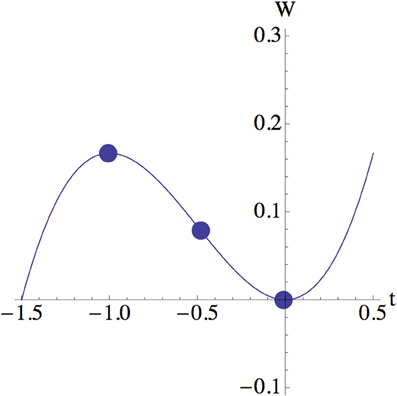
Figure 1. Solutions at g = 0.10.

FIGURE 2

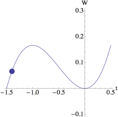
Figure 2. Solution at g = 1.0.

As g become larger, two larger roots become closer and annihilate beyond the critical value

$\begin{array}{ll}{g}_c=2^{-1/2}{3}^{-3/4}\simeq 0.31.& (40)\end{array}$

Figure 2 shows a placement of a root after the annihilation.

Analysis made here is merely a classical approximation and not full quantum treatment. Fortunately, we can integrate out one variable in the potential without relying on the saddle point approximation since present example is enough simple. Let us change the variables as

$\begin{array}{ll}u=\frac{t+\lambda }{2},v=\frac{t-\lambda }{2}.& (41)\end{array}$

Then, the partition function can be written as

$\begin{array}{lll}\hfill Z={\displaystyle \int }dudv\frac{1}{|2u+1|}exp\left\{\frac{1}{g^2}\left(-2W(u)-(2u+1)v^2\right)\right\}& & (42)\end{array}$

$\begin{array}{ll}={\displaystyle \int d}u\frac{1}{|2u+1{|}^{\frac{3}{2}}}\exp \left(-\frac{2}{g^2}W(u)\right)& (43)\end{array}$

where we performed Gaussian integral for v in the second line. Thus, we obtain one dimensional effective potential

$\begin{array}{ll}{V}_{e\mathrm{ff}}(u)=\frac{2}{g^2}W(u)+\frac{3}{2}log|2u+1|.& (44)\end{array}$

We note that the saddle point approximation corresponds to setting v = 0 in Equation (42), since we our choice of the saddle point, λ = t corresponds to it. Therefore,

$\begin{array}{ll}{V}_{\mathrm{saddle}}(u)=\frac{2}{g^2}W(u)+\frac{1}{2}log|2u+1|.& (45)\end{array}$

By comparing Equation (44) and Equation (45), we find that they only differ in the coefficient of the logarithmic term which is negligible for small g. Thus, the saddle point approximation works well for small coupling.

Finally, let us compare the shape of the potential for different values of g. Figure 3 is a plot of Equation (44) for small and large g. It is observed that the stable vacuum around u = 0 disappears for large g due to dominance of the logarithmic term. This phenomenon corresponds to the annihilation of saddle points which has already been observed in the saddle point analysis. Such dependence of the effective potential on the coupling is consistent with the fact that the D-brane describes the system at small coupling.

FIGURE 3

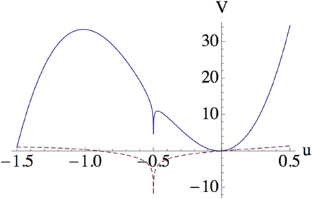
Figure 3. Effective potential for u, where solid line is a plot for g = 0.1 while dashed line is for g = 1.0.

4.2. N ≥ 2

Next we proceed to N ≥ 2, where the equations of motions are given by Equations (31) and (32). We again perform saddle point approximation by finding roots of these equations. The roots can be obtained numerically for each value of g. Numerical solutions for g = 0.01 and up to N = 3 are shown in Tables 1–3. We pick real roots only, and each solution is specified as (t, λ₁, …, λ_N). Due to the symmetry which exchanges λs, we only need to specify single configuration for each value of t among N permutations of λ. We also evaluate the value of effective potential V(λ, t) normalized by the value of D-brane tension 1/(6g²).

TABLE 1

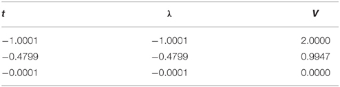
Table 1. Numerical solutions for N = 1 at g = 0.01.

TABLE 2

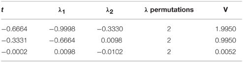
Table 2. Numerical solutions for N = 2 at g = 0.01.

TABLE 3

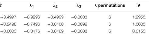
Table 3. Numerical solutions for N = 3 at g = 0.01.

We observe an interesting pattern in these results. Each root is located at one of a ‘site’ which is obtained by dividing the region −1 ≤ λ ≤ 0 into N + 1 intervals, i.e.,

$\begin{array}{lll}\hfill x_m=-\frac{m}{N+1},(m=0,1,\dots N+1).& & (46)\end{array}$

We also observe that the minimum value of t is given by −2/(N + 1) while values of λs can reach −1. We also observed that the sum of all eigenvalues are close to its value of potential, i.e.,

$\begin{array}{ll}t+{\displaystyle \sum _{a=1}^N}{\lambda }_a~V.& (47)\end{array}$

Finally, it is also interesting to see that the maximum value of the potential is close to 2 for all N.

We would like to close this subsection with a summary of our result:

• The stable vacuum is lost for large coupling. This indicates breakdown of D-brane description. The critical value of the coupling can be determined by saddle point equations.

• At small g, the local maximum of the effective potential is about twice higher than that of original one.

4.3. Large N

Let us evaluate the partition function in large N limit following with the standard method of matrix model (hep-th/0410165). We begin with the partition function

$\begin{array}{ll}Z={\displaystyle \int }d{\lambda }_{a}dt\frac{\prod _{a<b}{({\lambda }_a-{\lambda }_b)}^2}{\prod _a|t+{\lambda }_a+1|}{e}^{-\frac{1}{g^2}\left(W(t)+\sum _{a=1}^{N}W({\lambda }_a)\right)}& (48)\end{array}$

and introduce the t'Hooft coupling

$\begin{array}{ll}\mu =g^{2}N.& (49)\end{array}$

Then, saddle point equations read

$\begin{array}{ll}\frac{N}{\mu }(t+t^2)+{\displaystyle \sum _a}\frac{1}{{\lambda }_a+t+1}=0,& (50)\end{array}$

$\begin{array}{ll}\frac{N}{\mu }({\lambda }_a+{\lambda }_a^2)+\frac{1}{{\lambda }_a+t+1}-{\displaystyle \sum _b}\frac{2}{{\lambda }_a-{\lambda }_b}=0.& (51)\end{array}$

In large N limit, eigenvalues are described by a continuous distribution ρ(λ) and summation for eigenvalues is replaced with integration

$\begin{array}{ll}\frac{1}{N}{\displaystyle \sum _a}\to {\displaystyle \int }d\lambda \rho (\lambda ).& (52)\end{array}$

Then, saddle point equations are replaced with

$\begin{array}{ll}\frac{1}{\mu }(t+t^2)+{\displaystyle \int }d\lambda \frac{\rho (\lambda )}{t+\lambda +1}=0,& (53)\end{array}$

$\begin{array}{ll}\frac{1}{\mu }(\lambda +{\lambda }^2)+\frac{1}{N}\frac{1}{t+\lambda +1}-2{\displaystyle \int }d{\lambda }^{\prime }\frac{\rho ({\lambda }^{\prime })}{\lambda -{\lambda }^{\prime }}=0.& (54)\end{array}$

At leading order, the second term in Equation (54) becomes negligible. Thus, we obtain saddle point equations

$\begin{array}{ll}\frac{1}{\mu }(t+t^2)+{\displaystyle \int }d\lambda \frac{\rho (\lambda )}{\lambda +t+1}=0,& (55)\end{array}$

$\begin{array}{ll}\frac{1}{\mu }(\lambda +{\lambda }^2)-2{\displaystyle \int }d{\lambda }^{\prime }\frac{\rho ({\lambda }^{\prime })}{\lambda -{\lambda }^{\prime }}=0.& (56)\end{array}$

The latter equation (Equation 56) solves the planar limit of a cubic matrix model whose solution can be found elsewhere [28]. It is convenient to introduce the resolvent

$\begin{array}{ll}\omega (z)={\displaystyle \int }d\lambda \frac{\rho (\lambda )}{\lambda -z}.& (57)\end{array}$

The equation (Equation 56) can be replaced with an equation for ω(z). Once ω(z) is obtained, Equation (55) can be solved by finding solutions of

$\begin{array}{ll}\frac{1}{\mu }(t+t^2)+\omega (-t-1)=0.& (58)\end{array}$

The “one-cut” solution for the resolvent in large N limit is known to be [28]

$\begin{array}{ll}\omega (z)=\frac{1}{2\mu }\left\{z+z^2-\sqrt{(z-a)(z-b)}\left(1+\frac{a+b}{2}+z\right)\right\},& (59)\end{array}$

where a and b are endpoints of the branch cut, which define a support for the eigenvalue density ρ(λ). Requiring ω(z) ~ z⁻¹ at infinity, we obtain equations

$\begin{array}{ll}3{(a+b)}^2+4(a+b)-4ab=0,& (60)\end{array}$

$\begin{array}{ll}{(a+b)}^3+{(a+b)}^2-4ab(a+b+1)=16\mu .& (61)\end{array}$

which solve a and b as functions of μ. These equations are conveniently rewritten in terms of parameters σ = a + b and $\overline{\sigma }=a-b$ as

$\begin{array}{ll}16\mu =-\sigma (\sigma +1)(\sigma +2),& (62)\end{array}$

$\begin{array}{ll}2{(\sigma +1)}^2+\overline{\sigma }=2.& (63)\end{array}$

The latter equation restricts σ inside −2 ≤ σ ≤ 0. Further, Equation (62) tells us that there are no real roots of Equation (62) within −2 < σ < 1. Therefore, σ is constrained within

$\begin{array}{ll}-1\le \sigma \le 0.& (64)\end{array}$

Let us choose a brunch which starts from σ = 0. From Equation (62), the maximum value of μ reads

$\begin{array}{ll}{\sigma }_c=\frac{1}{3}(-3+\sqrt{3})~-0.42,{\mu }_c=\frac{1}{24\sqrt{3}}~0.024& (65)\end{array}$

Given these ingredients, Equation (55) can be rewritten into

$\begin{array}{ll}\frac{1}{\mu }\left\{\frac{3}{2}(t+t^2)+\frac{1}{2}\sqrt{t^2+(\sigma +2)t+\frac{3}{4}{\sigma }^2+2\sigma +1}\left(t-\frac{\sigma }{2}\right)\right\}=0.& (66)\end{array}$

Integrating this equation yields an effective potential for t,

$\begin{array}{ll}V(t)=\frac{1}{\mu }(v_1(t)+v_2(t))& (67)\end{array}$

where

$\begin{array}{ll}{v}_1(t)=\frac{3}{2}W(t),& (68)\end{array}$

$\begin{array}{ll}{v}_2(t)=\frac{1}{2}{{\displaystyle \int }}_0^{t}dz\left(z-\frac{\sigma }{2}\right)\mathrm{Re}\sqrt{z^2+(\sigma +2)z+\frac{3}{4}{\sigma }^2+2\sigma +1}.& (69)\end{array}$

A plot of effective potential (Equation 67) is shown in Figure 4. The local minimum at t = 0 and the local maximum around t = −1 are observed for any value of μ. This is consistent with the t'Hooft limit, in which g is small so that the D-brane description of the system holds. On the other hand, the height of the local maximum is always higher than that of the original potential W. The height is maximum for μ = 0; in this case, the potential is twice higher than W. While the height decreases as μ increases, it remains higher than W even at a maximum value of μ = μ_c. The increase of the height from the original one can be understood from the particle description of eigenvalues. Eigenvalues filled in the bottom of W(t) pull the tachyon t by attractive force. It makes harder for t to climb the potential wall, thus increases the height of the potential height. Such dependence of the effective potential on μ is quite different from that of the probe eigenvalue model investigated in Hanada et al. [29] where a plateau along the eigenvalue distribution is observed. The existence of the plateau is explained by the fact that a probe eigenvalue cannot be distinguished from others. Our model has no plateau since t can be distinguished from other eigenvalues.

FIGURE 4

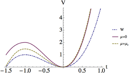
Figure 4. Effective potential at large N. The value of the potential is normalized by 1/(6μ). The original potential W(t) is shown together.

5. Conclusions and Discussions

In this paper, we proposed a systematic method to derive matrix models from level truncated OSFT. Obtained matrix model contains U(N) vectors and a scalar in addition to Hermite matrix. We have evaluated the effective potential of the scalar both for finite and large N. Increase of the potential height was observed at small coupling. In Section 3, we have interpreted our model as a system of ZZ branes and a ghost FZZT brane.

We would like to discuss further issues to be explored. First, we would like to present an alternative but rather heuristic interpretation of our result. Let us go back to the inverse of the determinant :

$\begin{array}{ll}det{(Q_{T0}+\varphi +\chi )}^{-1}.& (70)\end{array}$

The basic idea is that this quantity can be regarded as a propagator with ϕ and χ insertions. Recall that this factor is obtained by an integrating out χ_a and ${\overline{\chi }}_a$ which connect a D-brane with the tachyon vacuum where the world-sheet boundary disappears. Therefore, it is natural to think that Equation (70) amounts to a disk amplitude with single world-sheet boundary of a D-brane. Schematically, such disk amplitude can be written

$\begin{array}{ll}-Tr{\displaystyle \int }\frac{dt}{t}{e}^{-t(Q_{T0}+\varphi +\chi )}.& (71)\end{array}$

As is well known, small t limit of such amplitude corresponds to closed string propagation [30]. Therefore, the inverse determinant (Equation 70) encodes gravitational force between N D-branes and the tachyon vacuum⁹.

Second issue is abut the level truncation. We have seen that the approximated OSFT action at first few levels yields a one-matrix model which can be interpreted as c < 1 noncritical string theory [31]. It is interesting to improve the approximation by including higher level fields to obtain multi-matrix models. We speculate that that the improved matrix action continues to be dual to some closed string theory on more nontrivial background. Finally, we will recover original OSFT with infinitely many matrices in infinite level limit. We also expect that this matrix model describes a critical string theory in nontrivial background through AdS/CFT like duality [32]. Thus, the level truncated OSFT offers a way to describe closed strings in approximated geometry.

Last issue is the matrix description of OSFT based on the left-right splitting of open strings which have been examined in past [33–36]. Our model based on the KMTT decomposition looks quite differently from these models. However, as mentioned in the previous paragraph, our model will recover full OSFT in infinite level. Thus, the left-right splitting models and our model both describe same OSFT. We expect that all ingredients of KMTT, including Chan-Paton factors and regularized BCC projectors, are embedded in the left-right type matrix model in quite nontrivial manner.

Together with recent development which deals with different backgrounds as classical solutions [16], our result presents further evidence for SFT as a formulation of nonperturbative string theory. We hope that further developments in this direction will shed light on the landscape of string theory.

Author Contributions

The author confirms being the sole contributor of this work and approved it for publication.

Conflict of Interest Statement

The author declares that the research was conducted in the absence of any commercial or financial relationships that could be construed as a potential conflict of interest.

Footnotes

1. ^Each component field carries Chan-Paton indices.

2. ^As we will see later, extra vectors and scalars couple with the matrix. Here we omit them for simplicity.

3. ^We will ignore a constant shift in the action hereafter since it is not relevant for remaining discussions.

4. ^The open string field in universal sector is build from the Virasoro generator L_n and conformal ghosts b_n and c_n on the SL(2, R) vacuum [10].

5. ^This truncation makes sense if we replace Ψ_T with another representation of the tachyon vacuum solution, since we do not require its explicit form in following analysis.

6. ^A matrix model with U(N) vector was proposed in Klebanov et al. [22] in a different setting.

7. ^For example, see hep-th/0410165.

8. ^The ghost D-brane has been proposed as an object which cancels the effects of a D-brane [27].

9. ^This interpretation is consistent with the attractive force between λ and t observed in Section 3.

References

1. Witten E. Noncommutative geometry and string field theory. Nucl Phys. (1986) B268:253–94.

Google Scholar

2. Witten E. Chern-Simons gauge theory as a string theory. Prog Math. (1995) 133:637–678.

PubMed Abstract | Google Scholar

3. Dijkgraaf R, Vafa C. Matrix models, topological strings, and supersymmetric gauge theories. Nucl Phys. (2002) B644:3–20. doi: 10.1016/S0550-3213(02)00766-6

CrossRef Full Text | Google Scholar

4. Marino M. Chern-Simons theory, matrix integrals, and perturbative three manifold invariants. Commun Math Phys. (2004) 253:25–49. doi: 10.1007/s00220-004-1194-4

CrossRef Full Text | Google Scholar

5. Gaiotto D, Rastelli L. A Paradigm of open/closed duality: Liouville D-branes and the Kontsevich model. J High Energy Phys. (2005) 07:053. doi: 10.1088/1126-6708/2005/07/053

CrossRef Full Text | Google Scholar

6. Kontsevich M. Intersection theory on the moduli space of curves and the matrix Airy function. Commun Math Phys. (1992) 147:1–23.

Google Scholar

7. Takayanagi T, Terashima S. C=1 matrix model from string field theory. J High Energy Phys. (2005) 06:074. doi: 10.1088/1126-6708/2005/06/074

PubMed Abstract | CrossRef Full Text | Google Scholar

8. Ishibashi N, Kawai H. String field theory of noncritical strings. Phys Lett. (1993) B314:190–6.

Google Scholar

9. Fukuma M, Kawai H, Kitazawa Y, Tsuchiya A. String field theory from IIB matrix model. Nucl Phys. (1998) B510:158–74.

Google Scholar

10. Sen A. Universality of the tachyon potential. J High Energy Phys. (1999) 12:027.

Google Scholar

11. Sen A, Zwiebach B. Tachyon condensation in string field theory. J High Energy Phys. (2000) 03:002. doi: 10.1088/1126-6708/2000/03/002

PubMed Abstract | CrossRef Full Text | Google Scholar

12. Moeller N, Taylor W. Level truncation and the tachyon in open bosonic string field theory. Nucl Phys. (2000) B583:105–44. doi: 10.1016/S0550-3213(00)00293-5

CrossRef Full Text | Google Scholar

13. Gaiotto D, Rastelli L. Experimental string field theory. J High Energy Phys. (2003) 08:048. doi: 10.1088/1126-6708/2003/08/048

PubMed Abstract | CrossRef Full Text | Google Scholar

14. Kishimoto I, Takahashi T. Exploring vacuum structure around identity-based solutions. Theor Math Phys. (2010) 163:717–24. doi: 10.1007/s11232-010-0055-x

CrossRef Full Text | Google Scholar

15. Kishimoto I. On numerical solutions in open string field theory. Prog Theor Phys Suppl. (2011) 188:155–62. doi: 10.1143/PTPS.188.155

CrossRef Full Text | Google Scholar

16. Erler T, Maccaferri C. String Field Theory Solution for Any Open String Background. J High Energy Phys. (2014) 10:029. doi: 10.1007/JHEP10(2014)029

CrossRef Full Text | Google Scholar

17. Kishimoto I, Masuda T, Takahashi T, Takemoto S. Open string fields as matrices. Prog Theor Exp.Phys. (2015) 2015:033B05. doi: 10.1093/ptep/ptv023

CrossRef Full Text

18. Asano M, Kato M. New covariant gauges in string field theory. Prog Theor Phys. (2007) 117:569–87. doi: 10.1143/PTP.117.569

CrossRef Full Text | Google Scholar

19. Zeze S. Tachyon potential in KBc subalgebra. Prog Theor Phys. (2010) 124:567–80. doi: 10.1143/PTP.124.567

CrossRef Full Text | Google Scholar

20. Erler T, Schnabl M. A simple analytic solution for tachyon condensation. J High Energy Phys. (2009) 10:066. doi: 10.1088/1126-6708/2009/10/066

CrossRef Full Text | Google Scholar

21. Okawa Y. Comments on Schnabl's analytic solution for tachyon condensation in Witten's open string field theory. J High Energy Phys. (2006) 04:055. doi: 10.1088/1126-6708/2006/04/055

CrossRef Full Text | Google Scholar

22. Klebanov IR, Maldacena JM, Seiberg N. D-brane decay in two-dimensional string theory. J High Energy Phys. (2003) 07:045. doi: 10.1088/1126-6708/2003/07/045

CrossRef Full Text | Google Scholar

23. Kutasov D, Okuyama K, Park Jw, Seiberg N, Shih D. Annulus amplitudes and ZZ branes in minimal string theory. J High Energy Phys. (2004) 08:026. doi: 10.1088/1126-6708/2004/08/026

CrossRef Full Text

24. Fateev V, Zamolodchikov AB, Zamolodchikov AB. Boundary Liouville field theory. 1. Boundary state and boundary two point function (2000). arXiv:hep-th/0001012.

Google Scholar

25. Teschner J. Remarks on Liouville theory with boundary (2000). arXiv:hep-th/0009138.

Google Scholar

26. Zamolodchikov AB, Zamolodchikov AB. Liouville field theory on a pseudosphere (2001). arXiv:hep-th/0101152.

Google Scholar

27. Okuda T, Takayanagi T. Ghost D-branes. J High Energy Phys. (2006) 03:062. doi: 10.1088/1126-6708/2006/03/062

CrossRef Full Text | Google Scholar

28. Brezin E, Itzykson C, Parisi G, Zuber JB. Planar diagrams. Commun Math Phys. (1978) 59:35.

PubMed Abstract | Google Scholar

29. Hanada M, Hayakawa M, Ishibashi N, Kawai H, Kuroki T, Matsuo Y, et al. Loops versus matrices: the nonperturbative aspects of noncritical string. Prog Theor Phys. (2004) 112:131–81. doi: 10.1143/PTP.112.131

CrossRef Full Text | Google Scholar

30. Polchinski J. Dirichlet Branes and Ramond-Ramond charges. Phys Rev Lett. (1995) 75:4724–7.

PubMed Abstract | Google Scholar

31. Maldacena JM, Moore GW, Seiberg N, Shih D. Exact vs. semiclassical target space of the minimal string. J High Energy Phys. (2004) 10:020. doi: 10.1088/1126-6708/2004/10/020

CrossRef Full Text | Google Scholar

32. Maldacena JM. The Large N limit of superconformal field theories and supergravity. Int J Theor Phys. (1999) 38:1113–33. [Adv Theor Math Phys. (1998) 2:231].

Google Scholar

33. Rastelli L, Sen A, Zwiebach B. Half strings, projectors, and multiple D-branes in vacuum string field theory. J High Energy Phys. (2001) 11:035. doi: 10.1088/1126-6708/2001/11/035

CrossRef Full Text | Google Scholar

34. Gross DJ, Taylor W. Split string field theory. 1. J High Energy Phys. (2001) 08:009. doi: 10.1088/1126-6708/2001/08/009

PubMed Abstract | CrossRef Full Text | Google Scholar

35. Gross DJ, Taylor W. Split string field theory. 2. J High Energy Phys. (2001) 08:010. doi: 10.1088/1126-6708/2001/08/010

CrossRef Full Text | Google Scholar

36. Furuuchi K, Okuyama K. Comma vertex and string field algebra. J High Energy Phys. (2001) 09:035. doi: 10.1088/1126-6708/2001/09/035

CrossRef Full Text | Google Scholar