
- 1 Department of Electrical and Computer Engineering, Michigan State University, East Lansing, MI, USA
- 2 Department of Mechanical Engineering, University of Alberta, Edmonton, AB, Canada
A useful model of the arterial system is the uniform, lossless tube with parametric load. This tube-load model is able to account for wave propagation and reflection (unlike lumped-parameter models such as the Windkessel) while being defined by only a few parameters (unlike comprehensive distributed-parameter models). As a result, the parameters may be readily estimated by accurate fitting of the model to available arterial pressure and flow waveforms so as to permit improved monitoring of arterial hemodynamics. In this paper, we review tube-load model parameter estimation techniques that have appeared in the literature for monitoring wave reflection, large artery compliance, pulse transit time, and central aortic pressure. We begin by motivating the use of the tube-load model for parameter estimation. We then describe the tube-load model, its assumptions and validity, and approaches for estimating its parameters. We next summarize the various techniques and their experimental results while highlighting their advantages over conventional techniques. We conclude the review by suggesting future research directions and describing potential applications.
Introduction
Mathematical modeling of arterial hemodynamics has been longstanding. Two basic modeling approaches have been employed: forward modeling and inverse modeling. Forward modeling concerns building a model based on physical principles to predict data (i.e., estimating data from physical models with known parameters). This approach is useful for testing our understanding of the physiology underlying arterial hemodynamics. On the other hand, inverse modeling concerns building a model from observed data (e.g., estimating model parameters by fitting measured waveforms). Although less developed than its forward modeling counterpart, this approach is becoming more and more important by virtue of its ability to permit individualized monitoring of arterial hemodynamics.
The available models may be divided into two classes: lumped-parameter models and distributed-parameter models. The most popular lumped-parameter model is the “Windkessel” model proposed by Frank (Sagawa et al., 1990). It analogizes the arterial system as a capacitor connected in parallel with a resistor. The capacitor represents the large artery compliance, whereas the resistor represents the total peripheral resistance. This two-parameter Windkessel model can be extended to include additional circuit elements in order to improve accuracy (Stergiopulos et al., 1999). Because Windkessel models are so simple, they are highly suitable for parameter estimation purposes. That is, Windkessel models are characterized by only a few parameters, which can be readily estimated from the limited arterial waveforms typically available in practice. However, lumped-parameter models assume infinite pulse wave velocity and therefore cannot reproduce wave propagation and reflection phenomena that are essential in shaping these waveforms.
By contrast, distributed-parameter models can reproduce wave propagation and reflection phenomena through finite pulse wave velocity. Most often, distributed-parameter models represent the arterial system using a one-dimensional simplification of the Navier–Stokes equation. These models usually account for both geometrical and mechanical properties of the arteries explicitly as model parameters. Detailed distributed-parameter models have been built that account for multi-level branching, elastic and geometric tapering, and arterial terminations (Raines et al., 1974; Avolio, 1980; Zagzoule and Marc-Vergnes, 1986; Wan et al., 2002; Sherwin et al., 2003; Azer and Peskin, 2007; Huberts et al., 2009). These comprehensive models can provide great accuracy. However, the models cannot be readily applied for parameter estimation purposes, because they are characterized by an excessive number of model parameters that makes it virtually impossible to obtain unique parameter estimates from limited arterial waveforms.
Less accurate, yet mathematically tractable, distributed-parameter models have also been developed. These models usually consist of multiple tubes with terminal loads in parallel. Often times, the model comprises two such tubes and loads (“T-tube” model). The tube represents the wave propagation path in the large conduit arteries, whereas the load signifies the wave reflection site (e.g., arterial bed distal to a peripheral artery). The tube can be elastically and/or geometrically tapered or uniform as well as lossy (i.e., exhibits energy dissipation) or lossless, while the load can be non-parametric (i.e., characterized without a model structure through a generic frequency response) or parametric. It turns out that the simplest of these models, the uniform, lossless tube with parametric load, is almost as accurate as the most complicated of the models. Indeed, this model, which will henceforth be referred to simply as the tube-load model, is often able to fit arterial pressure and flow waveforms remarkably well despite being characterized by only a few parameters. Consequently, the tube-load model carries advantages of both Windkessel and comprehensive distributed-parameter models and therefore permits an attractive platform for improved monitoring of arterial hemodynamics.
In this paper, we review tube-load model parameter estimation techniques that have appeared in the literature for monitoring wave reflection, large artery compliance, pulse transit time, and central aortic pressure. We first provide a detailed explanation of the tube-load model and the estimation of its parameters. We then describe the various techniques and their experimental results while highlighting their advantages over conventional techniques. Table 1 provides a summary of the techniques. We conclude the review by suggesting future research directions and describing potential applications.
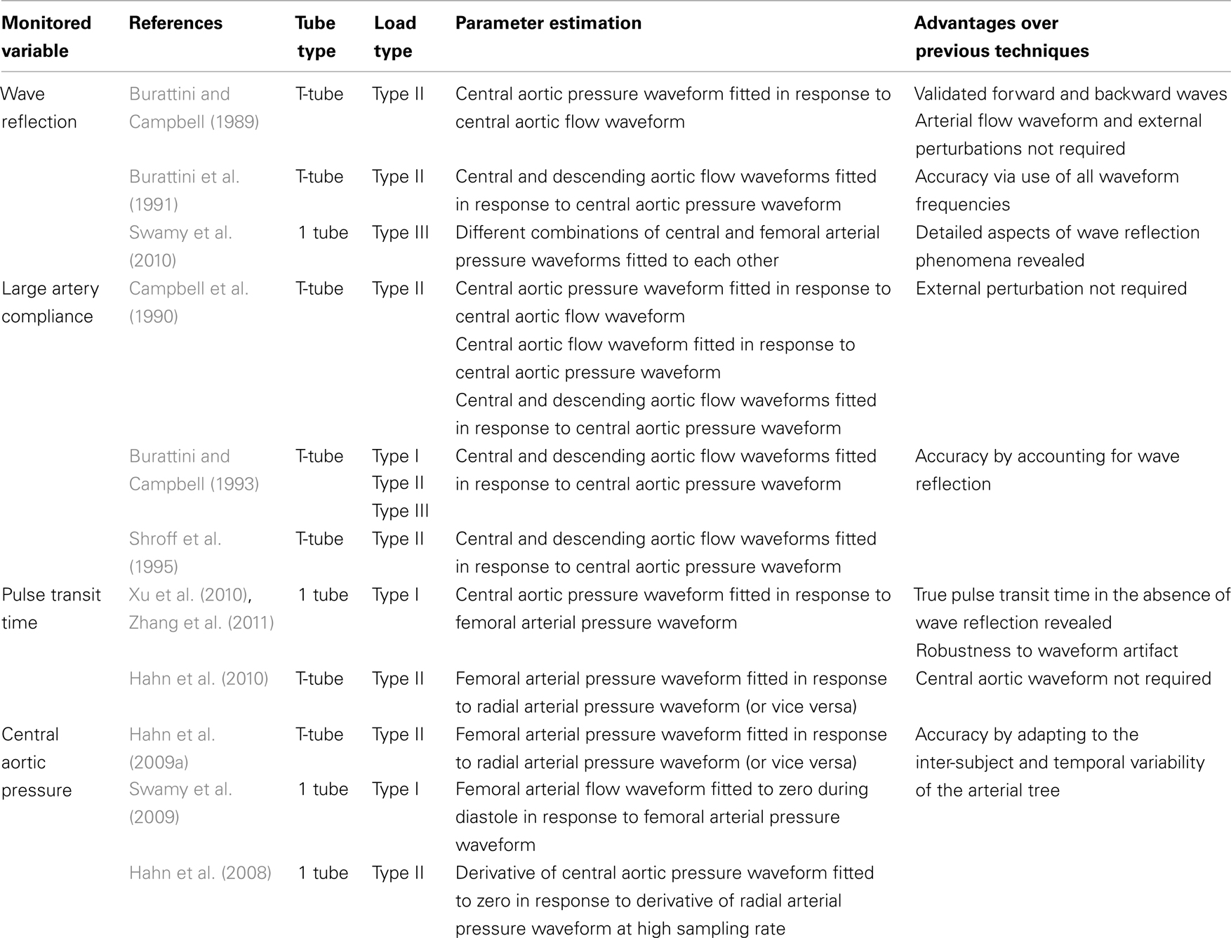
Table 1. Summary of available tube-load model parameter estimation techniques for monitoring arterial hemodynamics.
Tube-Load Model and Parameter Estimation
Model Description
Figure 1A illustrates the tube-load model. This model represents the arterial system as a parallel connection of m uniform, lossless tubes with parametric loads. The meaning of the tubes and loads depend on perspective. From the perspective of the central (ascending) aorta, a tube represents the wave propagation path through a segment of the aorta, whereas the load represents an effective reflection site due to the entire arterial network distal to the segment. For example, for the T-tube model in which m is equal to two, the two effective reflection sites correspond to the head-end and body-end arterial beds. The flow through the body-end tube represents the descending aortic flow, whereas the flow through the head-end tube represents the difference between central and descending aortic flows. From the perspective of a peripheral artery, on the other hand, a tube represents the wave propagation path from the central aorta to the peripheral artery, whereas the load represents the reflection site due to the arterial bed distal to the peripheral artery. In this case, m is equal to the number of peripheral arteries. The flow at the proximal end of a tube is not measurable. It represents the component of central aortic flow that reaches a peripheral artery. However, the sum of the flows at the proximal end of all tubes corresponds to the total central aortic flow.
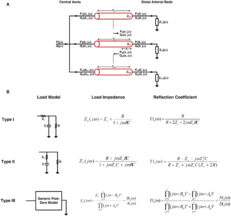
Figure 1. (A) The tube-load model with arbitrary load. (B) Three types of commonly used loads along with their corresponding impedances and reflection coefficients. See text for complete model details.
The ith tube is of length di and has constant characteristic impedance  , where li and ci are the large artery inertance and compliance, respectively. Pressure and flow waves propagate with constant time delay
  from one end of the tube to the other. Note that this time delay corresponds to pulse transit time and that its governing equation arises from the Bramwell–Hill equation (Bramwell, 1922). The mean value of the waves is constant throughout the tube.
The ith load has frequency-dependent impedance ZLi(jω), where j is the imaginary number and ω is the frequency, that is characterized by a pole–zero structure. Figure 1B shows three types of commonly used loads along with the specific form of their ZLi(jω). The Type I and Type II loads are three-parameter Windkessel models. These models account for the resistance R and compliance C of the effective load or peripheral resistance and compliance (depending on perspective) while matching the tube impedance at infinite frequency per arterial input impedance studies (Noordergraaf, 1978; Nichols and O’Rourke, 2005). The Type III load is a generic pole–zero model. A principal advantage of this type of model is that it allows a flexible system order rather than being fixed to first-order as with its Type I and Type II counterparts. The disadvantage is that it has no physiologic meaning. As a result, its coefficients are neither dependent on each other nor constrained as they are with the Type I and Type II loads. For any load, the wave reflection coefficient at the ith load is given by the following relationship involving tube and load impedances:
Qualitatively, pressure and flow waves propagate in the forward direction (proximal to distal tube ends) along a tube without distortion and are proportional to each other. These waves are reflected in the opposite direction at the load due to the impedance mismatch [Zci ≠ ZLi(jω)]. The resulting backward pressure and flow waves likewise propagate along the tube without distortion and are proportional to each other but have opposite sign. The actual arterial pressure and flow waveforms at any point on the tube then arise as the sum of the forward and backward propagating waves shifted in time to account for their wave propagation time to the point of interest.
Quantitatively, pressure and flow waves on a tube are related through its characteristic impedance as follows:

Here, Pf i(x, jω) and Pbi(x, jω) are forward and backward propagating pressure waves in the frequency-domain at a point x on the ith tube, and Qf i(x, jω) and Qbi(x, jω) are the corresponding flow waves at the same point. Note that the forward waves actually represent the sum of all waves propagating from the proximal to distal tube ends (i.e., the incident wave from the heart and the backward waves re-reflected at the heart), while the backward waves may be interpreted analogously. Also, note that x = 0 and x = di correspond to the distal and proximal ends of the tube, respectively.
The forward and backward waves at a distal tube end are related to each other through the wave reflection coefficient as follows:

The forward and backward waves at any point on a tube may be expressed in terms of the corresponding waves at the distal tube end as follows:
where the exponential term is the frequency-domain time shifting operator.
By combining Eqs 2–4, the actual arterial pressure and flow waveforms at any point on a tube may then be expressed in terms of the forward and backward waves as follows:
where Pi(x, jω) and Qi(x, jω) are the arterial pressure and flow waveforms in the frequency-domain at point x on the ith tube.
Due to the parallel connection of the model, the central aortic pressure waveform is identical to the arterial pressure waveforms at each proximal tube end, whereas the central aortic flow waveform is the sum of all flow waveforms at the proximal tube ends as follows:
where P(jω) and Q(jω) are the central aortic pressure and flow waveforms in the frequency-domain.
Finally, Eqs 5 and 6 may be given explicitly in terms of the tube-load model parameters by substituting a Γ(jω) from Figure 1B into these equations.
Assumptions and Validity
Assumptions of the tube-load model include: (a) wave propagation without energy loss in large conduit arteries, (b) a load characterized by a few parameters, and (c) non-interacting reflections occurring at distal sites only by virtue of neglecting elastic and geometric tapering and multi-level branching. Assumption (a) is quite valid. Friction in the large conduit arteries is indeed negligible, because resistance is inversely proportional to the fourth power of the vessel radius. Pressure loss in the descending aorta, for example, has been shown to be trivial (Burattini and Campbell, 2000). Assumption (b) is justifiable based on empirical data. That is, while the actual load is certainly complicated with many parameters needed for its representation, the arterial input impedance computed with the tube-load model has been shown to match that determined with standard non-parametric Fourier analysis (Burattini and Campbell, 1989, 1993). Note, however, that an even simpler purely real load may not be supported by empirical data (Burattini and Campbell, 2000). Assumption (c) is the least tenable but can be defended to some extent. The arterial terminations do often constitute the dominant reflection sites for two reasons. First, they pose the greatest impedance mismatch, as the radius of the arterioles is much smaller than that of proximal arteries (Pappano et al., 2007). Second, vessel tapering tends to be offset by vessel branching in the forward direction so as to achieve relative impedance matching (Noordergraaf, 1978). In addition, the tube-load model has been shown to fit experimental waveforms almost as well as an exponentially tapered version of the model (Fogliardi et al., 1997). On the other hand, backward waves should experience strong re-reflections as they return to the heart due to necessarily significant impedance mismatches in the backward direction (Noordergraaf, 1978). Further, the multiple reflected waves that return from distal sites actually interact in the aorta due to multi-level branching.
In short, the tube-load model has a physiologic foundation but does ignore aspects of actual arterial hemodynamics. Despite its simplicity, it is able to fit experimental arterial pressure and flow waveforms remarkably well. Figure 2 illustrates major waveform phenomena that the model can predict. This ability to fit experimental data provides further validation of the tube-load model and suggests that it may be phenomenological in addition to physiological.
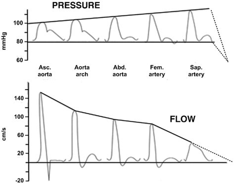
Figure 2. Experimental arterial pressure and flow waveforms with increasing distance from the heart. Reproduced from Nichols and O’Rourke (2005).
Parameter Estimation
Most often, estimating the tube-load model parameters is accomplished by casting the governing equations into a transfer function. The transfer function relating a pair of arterial pressure and/or flow waveforms at any points on a tube may be obtained based on Eq. 5. For example, using the T-tube model with Type II load, the transfer function relating the central aortic pressure waveform to the central aortic flow waveform is given as follows:
As another example, using the Type I load, the transfer function relating the central aortic pressure waveform to a peripheral arterial pressure waveform is given as follows:
The former transfer function is defined by the eight unknown parameters of the T-tube model. However, while the latter transfer function includes all four unknown model parameters of a single tube and load, only three aggregate parameters are actually observable (Ti, RiCi and ZciCi). Thus, all four parameters cannot be estimated, but identification of the transfer function is simplified to a three-parameter problem.
Estimation of the observable model parameters is accomplished in two steps. First, arterial pressure and flow waveforms corresponding to the input and output of the transfer function of interest are measured. Then, the parameters are estimated by finding the transfer function, which when applied to the measured input, optimally fits the measured output. Alternatively, in some instances, the parameters of the transfer function may be optimally estimated using a priori physiologic knowledge (see Pulse Transit Time Monitoring and Central Aortic Pressure Monitoring). The advantage of this alternative is to reduce the burden on the required waveform measurements. In either case, parameter estimation is usually performed in the time-domain by converting the transfer function into a recursive difference equation, and the optimality is typically established in the least squares sense.
The step of estimating the tube-load model parameters is actually quite challenging. First, the transfer functions are not simply linear in distinct parameters. For example, as can be ascertained from Eqs 7 and 8, the transfer functions are non-linear in the Ti (pulse transit time) parameter. Second, the parameter values have numerical constraints. For instance, the characteristic impedance should be smaller than the peripheral resistance, and all parameters must be positive and not exceed physiologic bounds. For these two reasons, straightforward parameter estimation techniques with analytical solutions are generally not applicable. The parameters are instead typically estimated via numerical search in which the needed global optimum cannot be guaranteed. Use of brute-force methods that search over a discretized grid in multi-dimensional parameter space increases the likelihood of identifying the global optimum at the expense of substantial computational time. On the other hand, use of available local search methods such as the steepest descent method, conjugate gradient method, Newton’s method and its Levenberg–Marquardt modification, and simplex method (possibly with penalty factors for keeping the parameters within physiologic bounds; Ljung, 1999) require little computational time, but the global optimum is seldom found without an initial guess that resides near the global optimum. This problem is often mitigated by employing multiple, initial guesses and then choosing the solution that represents the optimum amongst the multiple solutions of the local search method. However, the computational time will obviously increase with the number of initial guesses. Another practical issue is that the upper physiologic bounds on the parameters are often unclear. However, the challenge of parameter estimation can be alleviated to some degree by direct measurement of one or more parameters, especially pulse transit time and load resistance (Campbell et al., 1990; Burattini and Campbell, 1993; Hahn et al., 2009a; Swamy et al., 2009). Despite these challenges, asymptotic variance analysis has shown that the confidence intervals on the parameters estimates can be tight (Hahn et al., 2009a).
Wave Reflection Monitoring
Significance
The magnitude and timing of the backward wave relative to the forward wave in the central aorta can materially impact cardiac afterload and myocardial perfusion. For example, a significant reflected wave returning early from distal sites to the aorta during systole can impede stroke volume, whereas such a wave arriving later during diastole can augment myocardial perfusion. It would therefore be useful to be able to precisely monitor wave reflection.
Previous Techniques
Several techniques are available to separate arterial pressure and flow waveforms into their forward and backward wave components. The most popular of these techniques (Westerhof et al., 1972) models the proximal aorta as a short, uniform, lossless tube. The tube characteristic impedance is then estimated from measured central aortic pressure and flow waveforms as the average magnitude of the high frequency arterial input impedance. Finally, the forward and backward pressure waves in the tube are calculated from the central aortic pressure and flow waveforms and the characteristic impedance by adding pressure waves and subtracting flow waves (i.e., solution of two equations with two unknowns that arise from Eqs 2 and 5).
A couple of techniques are also available to calculate forward and backward waves from arterial pressure waveforms alone. The most interesting of these techniques (Newman et al., 1979) measures an arterial pressure waveform before and after complete occlusion of a distal artery. The backward pressure wave is then determined as half of the waveform obtained after the occlusion. Finally, the forward pressure wave is determined by subtracting this backward wave from the waveform obtained before the occlusion.
While these techniques have shed light on wave reflection phenomena, they have several disadvantages. First, it is generally difficult to validate the calculated waves against reference measurements. Indeed, to our knowledge, the techniques have yet to be validated in this way. Second, these techniques require either an arterial flow waveform, which is more difficult to measure than arterial pressure waveforms, or an experimental perturbation and are therefore not convenient to implement. Third, the estimation of characteristic impedance can be problematic. For example, the waveforms usually lack sufficient high frequency content. Finally, detailed aspects of wave reflection phenomena such as the location of the effective reflection sites cannot be ascertained with these techniques.
Tube-Load Model Parameter Estimation Techniques
Wave reflection can be readily monitored using tube-load model parameter estimation techniques. Once the model parameters are estimated from measured waveforms, the forward and backward waves can be determined. In particular, based on Eq. 5, the forward wave can be calculated from the parameter estimates and measured waveforms using standard deconvolution methods (Proakis and Manolakis, 2007). Then, according to Eq. 3, the backward wave can be computed from the forward wave and parameter estimates via convolution. Because these techniques are based on a model of the arterial system, they are able to overcome the disadvantages of the previous techniques enumerated above. First, the calculated waves can be validated in terms of their ability to predict a reference arterial pressure or flow waveform not utilized for parameter estimation (by adding or subtracting the waves after time shifting to account for the wave propagation time to the reference measurement site). Second, the waves can be calculated from only arterial pressure waveforms obtained without any external perturbation. Third, the model parameters can be estimated more accurately by the analysis of all waveform frequencies. Finally, the model parameters reveal detailed aspects of wave reflection phenomena. These advantages come at the cost of using a model that is not entirely correct (see Tube-Load Model and Parameter Estimation).
Burattini and Campbell (1989) calculated forward and backward waves from central aortic pressure and flow waveforms, validated the waves, and estimated the locations of the effective reflection sites. The authors specifically utilized the T-tube model with Type II load. They determined the load resistance parameters from measured total peripheral resistance and an assumed ratio of the head-end to body-end arterial flows. Then, based on Eq. 7b, they estimated the remaining six parameters by fitting the central aortic pressure waveform in response to the central aortic flow waveform. The waveform fitting was always satisfactory. From the model parameter estimates and Eq. 7a, they also predicted the descending aortic flow waveform. This prediction is equivalent to subtracting the calculated forward and backward waves at the proximal end of the body-end tube. Figure 3 illustrates that the predicted waveform corresponded quite well to the measured descending aortic flow waveform. The authors analyzed the validated forward and backward waves. A prominent oscillation observed in the central aortic pressure waveform during diastole was caused by reflection from the body-end. Based on phase velocity estimated with the descending aortic flow waveform, the effective body-end reflection site is located at abdominal aorta. Finally, the effective head-end reflection site is closer to the heart and responsible for reflection during late systole. Later, these authors (Burattini and Campbell, 1993) would confirm that the abdominal aorta represents the effective body-end reflection site using similar techniques and further validate the waves via prediction of the waveform at this site (see Large Artery Compliance Monitoring).
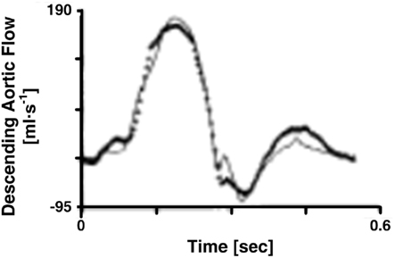
Figure 3. Descending aortic flow waveforms measured (line with crosses) and predicted (solid line) from central aortic pressure and flow waveforms. Adapted from Burattini and Campbell (1989).
Burattini et al. (1991) calculated forward and backward waves to investigate the existence of two distinct reflection sites. The authors specifically used the T-tube model with Type II load and measured the load resistance parameters. Based on Eq. 7a, they estimated the remaining six model parameters by fitting the central and descending aortic flow waveforms in response to the central aortic pressure waveform. Three waveforms were used in accordance with an earlier study by the authors (Campbell et al., 1990; see Large Artery Compliance Monitoring). They analyzed the forward and backward waves when a diastolic oscillation was present and absent in the central aortic pressure waveform. Two effective reflection sites could explain either case. When the diastolic oscillation was present, both reflection sites were needed to fit the oscillation. When this oscillation was absent, the backward waves from the head-end and body-end either canceled each other out or superimposed on each other to appear as a single backward wave. In this case, one tube and load sufficed in fitting the central aortic pressure waveform. Figure 4 illustrates the forward and backward waves calculated during both cases. In short, there are two reflection sites, but they can sometimes appear as one to the heart.
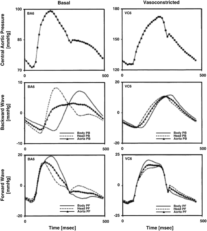
Figure 4. Measured central aortic pressure waveforms and forward and backward pressure waves in the central aorta (PF and PB) calculated from central aortic pressure and flow and descending aortic flow waveforms. Adapted from Burattini et al. (1991).
Swamy et al. (2010) calculated forward and backward waves from just two arterial pressure waveforms and validated the resulting waves during diverse hemodynamic interventions. The authors specifically employed a single tube with Type III load to relate central aortic and femoral arterial pressure waveforms and used the foot-to-foot detection technique to estimate the pulse transit time parameter (see Pulse Transit Time Monitoring). They re-cast Eq. 5with Type III load to the following form:
The waveforms X(jω) and Y(jω) can be easily constructed from the measured waveforms. Given these constructed waveforms, Eq. 9may be regarded as linear in distinct parameters for one-step ahead fitting (i.e., fitting the output in response to the past values of the input and output rather than fitting the entire output in response to the input as described in Tube-Load Model and Parameter Estimation). They therefore employed standard autoregressive exogenous input identification (Ljung, 1999) to analytically estimate the parameters as well as to determine the order of the wave reflection coefficient and thus the load (see Figure 1B). Rather than using standard deconvolution to calculate two versions of the forward wave from Eq. 5and each arterial pressure waveform, they computed a single, optimal forward wave from both waveforms using multi-channel linear least squares deconvolution (Abed-Meraim et al., 1997). From the calculated forward and backward waves, the authors predicted the abdominal aortic pressure and femoral arterial flow waveforms (wherein the appropriate time shift was established by again using the foot-to-foot detection technique to estimate the pulse transit time between the corresponding measured waveform and the femoral arterial pressure waveform). Figures 5A,B illustrate that the predicted waveforms agreed well with the corresponding measured waveforms. As further validation, Figure 5C shows that the magnitude of the backward wave relative to the forward wave correctly increased during vasoconstriction and decreased during vasodilation. Finally, the estimated load order was second-order on average. This finding indicates that the first-order Types I and II loads are reasonable choices.
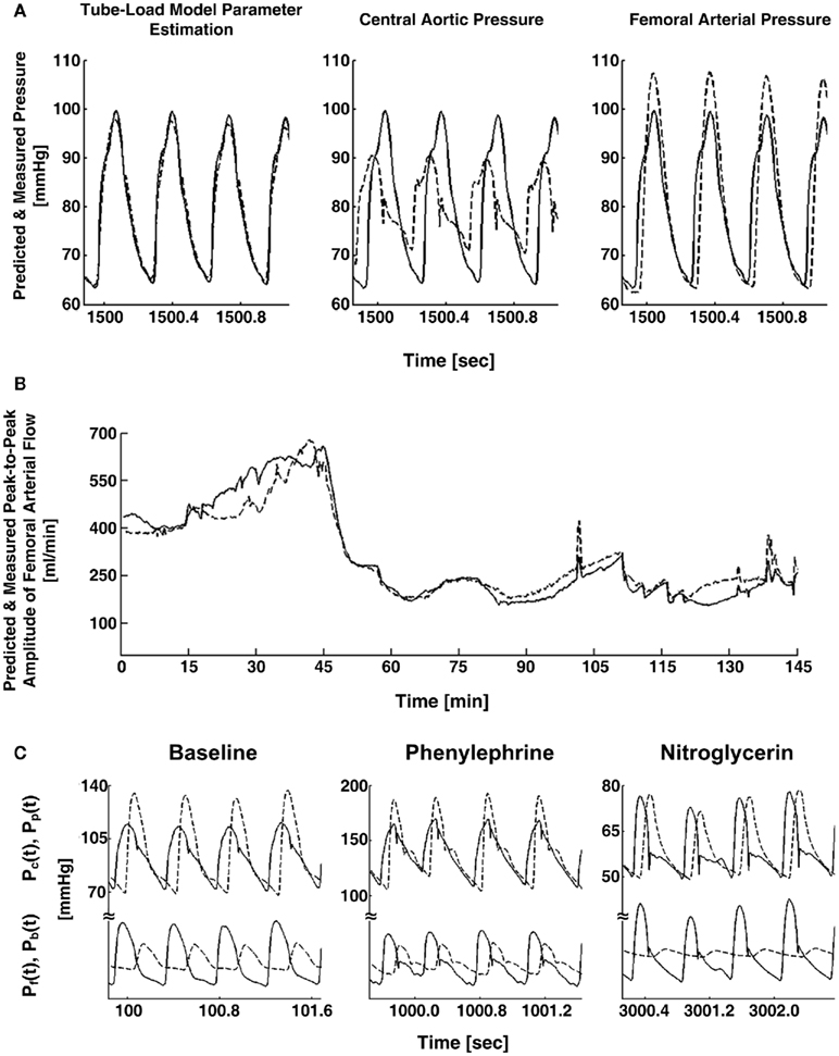
Figure 5. (A) Abdominal aortic pressure waveforms measured (solid) and predicted (dash) from central aortic and femoral arterial pressure waveforms (left) and the raw central aortic and femoral arterial pressure waveforms (center and right). (B) Femoral arterial flow measured (solid) and predicted (dash; after a single calibration) from central aortic and femoral arterial pressure waveforms during several interventions. (C) Measured central aortic [Pc(t), solid] and femoral arterial [Pp(t), dash] pressure waveforms (upper) and forward [Pf(t), solid] and backward [Pb(t), dash] waves in the central aorta (lower) calculated from the measured waveforms. Adapted from Swamy et al. (2010).
Large Artery Compliance Monitoring
Significance
Large artery compliance characterizes arterial stiffness. The decline in this parameter is a major part of the degenerative changes that occur in aging and arterial disease (Haynes et al., 1979; Benetos et al., 1993; Van Bortel and Spek, 1998; Lévy, 2001). Indeed, in hypertension, the age-matched increase in pulse pressure is mainly due to a decrease in large artery compliance caused in part by intrinsic alteration of the arterial wall (London et al., 1989; Reneman and Hoeks, 1995). Thus, large artery compliance is of great clinical value. For example, it has been shown to be able to sensitively discriminate the severity of coronary artery disease (Waddell et al., 2001), and early recognition of abnormal compliance may favor patients at risk for arterial disease (Glasser et al., 1998). In addition, the ability to monitor large artery compliance is important for advancing the understanding of its role in pathophysiology.
Previous Techniques
The gold standard technique for monitoring large artery compliance is to measure aortic volume (or cross-sectional area) and pressure during an external perturbation (e.g., vena cava balloon occlusion) and then determine the slope of the line that best relates the resulting changes in volume to pressure. However, this technique is difficult to implement. More convenient techniques are available in which large artery compliance is estimated from arterial pressure and flow waveforms without the need for any external perturbation. The simplest of these techniques is the ratio of the stroke volume to pulse pressure (Hamilton and Remington, 1947). Another popular technique is the diastolic decay time method in which the RC time constant of the Windkessel model is estimated from an arterial pressure waveform during diastole and then divided by the ratio of the average arterial pressure to cardiac output (Sagawa et al., 1990). However, these waveform analysis techniques are subject to limited reliability, because they neglect wave reflection phenomena.
Tube-Load Model Parameter Estimation Techniques
Large artery compliance can also be monitored from pressure and flow waveforms using tube-load model parameter estimation techniques. These techniques specifically calculate large artery compliance by dividing the estimated pulse transit time parameter ( ) by the estimated characteristic impedance parameter (
 ). Their obvious advantage over the previous waveform analysis techniques is taking wave reflection into account.
Campbell et al. (1990) compared large artery compliance and other parameter estimates of different waveform analysis techniques during three vasoactive states. The authors specifically used the T-tube model with Type II load and measured the load resistance parameters. Based on Eq. 7, they estimated the remaining six model parameters by fitting (a) the central aortic pressure waveform in response to the central aortic flow waveform, (b) the central aortic flow waveform in response to the central aortic pressure waveform, and (c) the central and descending aortic flow waveforms in response to the central aortic pressure waveform. In all cases, the model was able to fit the waveforms well. Figure 6A illustrates an example of the waveform fitting. However, tight confidence intervals on the parameter estimates were only obtained when all three waveforms were analyzed. They justified this finding by arguing that the descending aortic flow waveform carries additional information revealing distinct reflection characteristics associated with the body-end arterial system and thus advocated the use of three waveforms for estimating the T-tube model. Further, the resulting large artery compliance estimates (and other parameter estimates) were consistent with known physiology. That is, the body-end compliance was greater than the head-end compliance. Indeed, the body-end consists of the most compliant arterial vessels (e.g., thoracic aorta) and has a greater vascular network. In addition, both compliances decreased with vasoconstriction and increased with vasodilation, as expected. Finally, Figure 6B shows that the sum of the two compliances was consistently smaller than that estimated with the Windkessel model during the three vasoactive states. Thus, accounting for wave reflection does make a difference in estimating large artery compliance.
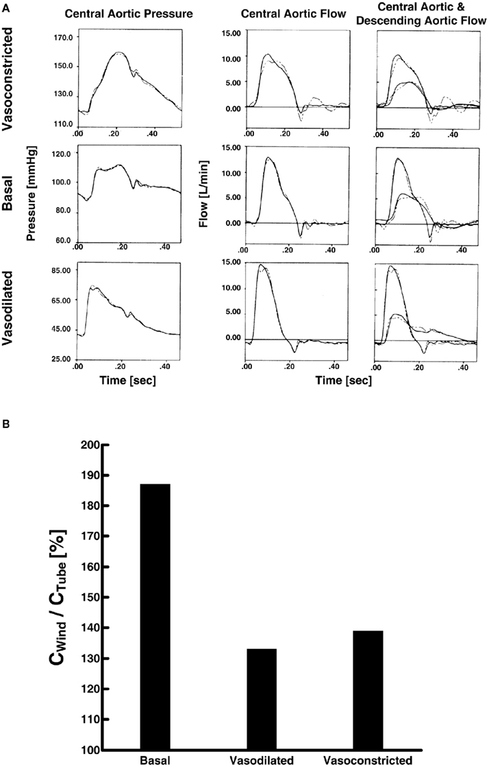
Figure 6. (A) Measured central aortic pressure and flow and descending aortic flow waveforms (solid) and waveforms fitted (dash) using the first two waveforms only (left and center) and all three waveforms (right). Adapted from Campbell et al. (1990). (B) Ratio of large artery compliance estimates via Windkessel model (CWind) and tube-load model (CTube; Campbell et al., 1990).
Burattini and Campbell (1993) validated the large artery compliance estimates against gold standard reference measurements. The authors specifically estimated the parameters of the T-tube model with all three load types by fitting the central and descending aortic flow waveforms in response to the central aortic pressure waveform as per Campbell et al. (1990). They then used pulse wave velocity measurements via the foot-to-foot detection technique (see Pulse Transit Time Monitoring) to conclude that the distal end of the body-end tube corresponds to the abdominal aorta. The estimated compliance of the body-end tube was very close to the reference measurements obtained from the aortic arch to the abdominal aorta (123 ± 20 × 10−6 g −1 cm−4 s2 versus 119 ± 10 × 10−6 g−1 cm−4 s2). On the other hand, they did not find physiologic meaning in the compliance estimates of the load model and therefore advocated the use of the Type III load. The authors also validated the model as a whole by predicting the abdominal aortic pressure waveform from the model parameter estimates and Eq. 8for the body-end tube and load (see Wave Reflection Monitoring). The predicted waveform was in good agreement with the pressure waveform measured at the abdominal aorta.
Shroff et al. (1995) investigated the ability of the model parameter estimates to track changes during local as well as global interventions, with emphasis on arterial compliance. The authors employed the same parameter estimation technique as Campbell et al. (1990). For a local intervention, they inflated a balloon in the iliac artery. The body-end tube compliance and all of the head-end model parameters were not affected by this intervention, whereas the compliance and resistances of the body-end load were significantly altered. Figure 7 illustrates these physiologically consistent results. For global interventions, they administered a vasoconstrictor and vasodilator. The compliances and other model parameters changed in the expected direction in response to these interventions similar to Campbell et al. (1990). However, one notable difference was that the head-end tube compliance did not change during vasodilation.
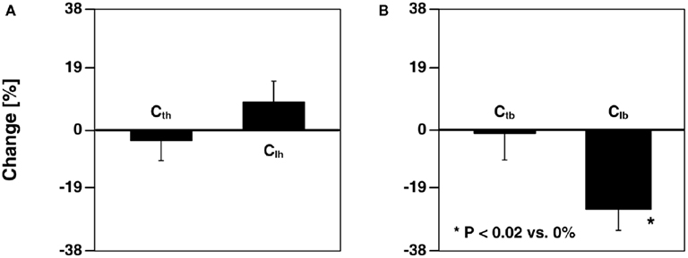
Figure 7. Percent changes in (A) head-end tube and load compliances (Cth and Clh) and (B) body-end tube and load compliances (Ctb and Clb) estimated from central aortic pressure and flow and descending aortic flow waveforms after inflation of a balloon in the left external iliac artery. Adapted from Shroff et al. (1995).
Pulse Transit Time Monitoring
Significance
As indicated above, pulse transit time varies with the square root of large artery compliance. Indeed, pulse transit time, in the form of pulse wave velocity, is now the most popular index of arterial stiffness for two reasons. First, it is an independent predictor of all-cause mortality and cardiovascular events in hypertensive and other patients (Mancia et al., 2007). Second, it can be estimated from only arterial pressure waveforms, whereas direct estimation of large artery compliance requires more difficult arterial flow waveform measurements.
Previous Techniques
Conventionally, pulse transit time is estimated by measuring central and peripheral arterial pressure waveforms with non-invasive transducers and then detecting the foot-to-foot time delay between the waveforms. The premise of this foot-to-foot detection technique is that interference from the backward wave is negligible during late diastole and early systole when the waveform feet occur. However, wave reflection interference may not always be trivial at the waveform feet. For example, at low heart rate, the backward wave adds constructively to the forward wave. Thus, in this condition, the technique can grossly underestimate pulse transit time. Just as important, the technique is not robust to artifact often present in the non-invasive waveforms (Solà et al., 2010). These two disadvantages of the foot-to-foot detection technique prevent pulse transit time from realizing its potential clinical value. Moreover, in contrast to peripheral arterial pressure waveforms, central arterial pressure waveforms are actually not easy to measure (Chen et al., 1997). As a result, pulse transit time is not widely used in clinical practice (Mancia et al., 2007).
Several other techniques are available for estimating pulse transit time/pulse wave velocity. However, for the most part, these techniques have not revealed any practical advantage over the foot-to-foot detection technique. As a relevant example, techniques have been conceived for estimating the true pulse transit time (i.e., the pulse transit time in the absence of wave reflection) via a tube model with a non-parametric load (see Milnor, 1989 and references therein). However, these techniques are inconvenient in that they necessitate three or more waveforms for measurement.
Tube-Load Model Parameter Estimation Techniques
Monitoring pulse transit time with tube-load model parameter estimation techniques potentially has significant advantages over the previous techniques. Since the model includes the true pulse transit time as an explicit parameter and characterizes the load with only a few parameters, these techniques can yield an artifact-robust estimate of the pulse transit time in the absence of wave reflection from only central and peripheral arterial pressure waveforms or even a pulse transit time estimate from just two peripheral arterial pressure waveforms.
Xu et al. (2010) and Zhang et al. (2011) estimated pulse transit time from central and peripheral arterial pressure waveforms during cardiac pacing and various other hemodynamic interventions. The authors specifically employed a single tube with Type I load. Based on Eq. 8, they estimated the true pulse transit time and the other two observable parameters by fitting the central aortic pressure waveform in response to a femoral arterial pressure waveform. Since the entire waveforms, rather than just their feet, were analyzed, they claimed that these pulse transit time estimates would be more robust to artifact in addition to reflecting the pulse transit time in the absence of wave reflection. To support this claim, the authors compared the tube-load model parameter estimation technique to the foot-to-foot detection technique in terms of the ability of their pulse transit time estimates to track changes in arterial pressure, a major, acute determinant of aortic stiffness with an inverse relationship to arterial compliance. The tube-load model parameter estimation technique showed tighter correlation between the pulse transit time estimates and arterial pressure than the foot-to-foot detection technique, especially during low signal-to-noise and low heart rate conditions. Figure 8 illustrates that the tube-load model parameter estimation technique revealed strong, negative correlation at low heart rates, whereas the conventional technique showed non-physiologic, positive correlation indicative of increasing underestimation of pulse transit time with decreasing heart rate.
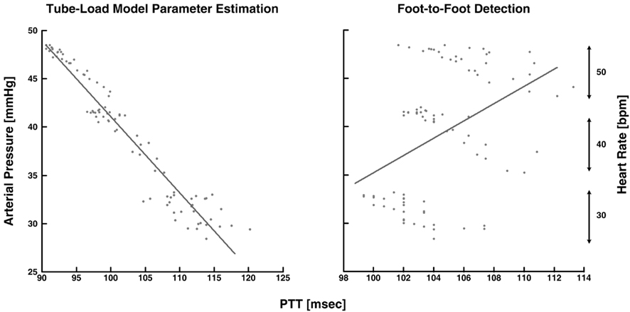
Figure 8. Measured arterial pressure versus pulse transit time (PTT) estimated from central aortic and femoral arterial pressure waveforms. Adapted from Zhang et al. (2011).
Hahn et al. (2010) estimated pulse transit time from two diametric peripheral arterial pressure waveforms measured at the radial and femoral arteries. The authors specifically employed a T-tube model with Type II load. To estimate the model parameters without using the central aortic pressure waveform, they assumed that the head-end and body-end effective reflection sites correspond to the arterial beds distal to the radial and femoral arteries, respectively. They used Eq. 8to define the transfer functions relating the central aortic pressure waveform to the radial and femoral arterial pressure waveforms as follows:
where the subscripts 1 and 2 denote the radial and femoral arteries, respectively. The authors were then able to estimate the true pulse transit time parameters and the other four observable parameters by fitting the femoral arterial pressure waveform in response to the radial arterial pressure waveform (or vice versa) via the second equality in Eq. 10. To facilitate the parameter estimation, they constrained the pulse transit times so that their difference is equal to the foot-to-foot time delay between the radial and femoral arterial pressure waveforms. It is important to note that Eq. 10may only be used to estimate the model parameters, if the transfer functions on the left- and right-hand sides of Eq. 10do not share any poles or zeros (i.e., the coprime condition Doyle et al., 2009). That is, common poles and/or zeros would cancel each other out, and the associated parameters would become unobservable in Eq. 10. In addition to the coprime condition, the authors showed in earlier work (Hahn et al., 2009a) that additional conditions must be met in order to uniquely estimate the parameters in Eq. 10. They further showed that these conditions can be fulfilled by appropriate choice of the peripheral arterial measurement sites and sampling frequency. The estimated pulse transit time was highly correlated with the foot-to-foot time delay between the central aortic (end of aortic arch) and peripheral arterial pressure waveforms. Figure 9 shows the estimates (after an initial calibration with the foot-to-foot time delay) versus the foot-to-foot time delays.
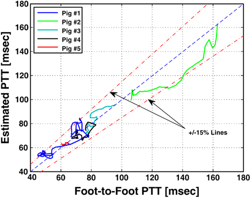
Figure 9. Pulse transit time estimated from radial and femoral arterial pressure waveforms (after a single calibration) versus PTT estimated from aortic and peripheral arterial pressure waveforms via foot-to-foot detection. Adapted from Hahn et al. (2010).
Central Aortic Pressure Monitoring
Significance
Systolic and diastolic pressures measured specifically in the central aorta truly reflect cardiac afterload and myocardial perfusion. Further, pressure exerted on the central (elastic) arteries, as opposed to the peripheral arteries, is a major determinant of the degenerative changes that occur in hypertension and aging (Agabiti-Rosei et al., 2007). Because of its greater physiologic relevance, central arterial pressure can provide superior clinical value. Indeed, central arterial pressure, but not peripheral arterial pressure, has been shown to be an independent predictor of morality and/or cardiovascular events in geriatric patients (Pini et al., 2008), end-stage renal disease patients (Safar et al., 2002), and coronary artery disease patients (Jankowski et al., 2008). Moreover, compared to peripheral arterial pressure, central arterial pressure has been shown to correlate more strongly with age (Choi et al., 2010) and better discriminate the severity of coronary artery disease (Waddell et al., 2001). However, peripheral arterial pressure waveforms can be measured more easily and safely and are therefore typically measured in practice. Thus, it would be of great value to be able to monitor central aortic pressure from peripheral arterial pressure.
Previous Techniques
Several generalized transfer function techniques are available for deriving the central aortic pressure waveform from a peripheral arterial pressure waveform (Karamanoglu et al., 1993; Chen et al., 1997; Fetics et al., 1999; Söderström et al., 2002; Hope et al., 2003). These techniques involve creating an average black-box (rather than physiology-based) transfer function using central aortic and peripheral arterial pressure waveform measurements from a group of subjects and then applying this transfer function to the peripheral arterial pressure waveform of a new subject to predict the central aortic pressure waveform. The techniques therefore do not adapt to the inter-subject and temporal variability of the arterial tree due to, for example, age-related large artery compliance differences and neuro-humoral modulation of peripheral resistance, and consequently may be prone to serious error.
To improve accuracy, a technique to adapt the transfer function to arterial parameters has become available more recently (Sugimachi et al., 2001). This technique defines the transfer function in terms of the tube-load model parameters (i.e., inverse of Eq. 8). The pulse transit time parameter is then measured for each subject using a non-invasive measurement of any waveform indicative of the timing of the central arterial pulse. However, similar to generalized transfer function techniques, this technique uses population averages for the remaining observable parameters and is therefore only mildly adaptive.
Tube-Load Model Parameter Estimation Techniques
The central aortic pressure waveform can also be monitored from peripheral arterial pressure waveforms using tube-load model parameter estimation techniques. These techniques estimate all observable transfer function model parameters by exploiting a priori physiologic knowledge. Thus, the resulting transfer functions are fully adaptive by virtue of continually re-estimating the model parameters for each subject.
Hahn et al. (2009a) derived the central aortic pressure waveform from radial and femoral arterial pressure waveforms. The authors specifically employed a T-tube model with Type II load, as opposed to a black-box model (Swamy et al., 2007; Swamy and Mukkamala, 2008). They estimated the model parameters based on Eq. 10in accordance with their parallel work (see Pulse Transit Time Monitoring). Then, they derived the central aortic pressure waveform by deconvolving the peripheral arterial pressure waveforms from the resulting transfer functions in Eq. 10using a filtering technique they developed for stable deconvolution of signals in multi-channel coprime systems. In addition to the central aortic pressure waveform, the authors used the model parameter estimates to derive the central aortic flow waveform. Figure 10A shows a block diagram of their derivation of the central aortic pressure and flow waveforms. They specifically used the six estimated parameters and the RC time constant, as determined from the peripheral arterial pressure waveforms during diastole, to determine all but one of the parameters of the transfer function in Eq. 7b. They were then able to apply this transfer function to the derived central aortic pressure waveform to estimate the contour of the central aortic flow waveform (i.e., without absolute gain factor). Finally, the authors developed a metric that correlates with the quality of the estimated T-tube model parameters. The metric is defined as the distance between the heart rate frequency and the frequency at which the transfer function of the body-end tube model in Eq. 10achieves its first maximum modulus. The rationale is that the fidelity of the parameter estimates depends on how well the arterial pressure waveforms (with maximum energy located at the heart rate frequency) excites the arterial tree at the first maximum modulus frequency (where the T-tube model is highly sensitive to all of the observable model parameters). Figure 10B illustrates that the derived central aortic pressure and flow waveforms (the latter after an initial calibration) agreed well with the corresponding measured waveforms.
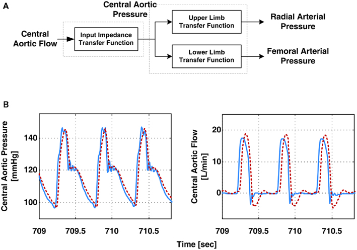
Figure 10. (A) Block diagram of derivation of the aortic pressure and central aortic flow waveforms from radial and femoral arterial pressure waveforms. (B) Measured (solid) and derived (dash) waveforms. Adapted from Hahn et al. (2009a).
Swamy et al. (2009) derived the central aortic pressure waveform from a single peripheral arterial pressure waveform during diverse hemodynamic interventions. The authors specifically employed a single tube with essentially Type I load to relate a peripheral arterial pressure waveform to the central aortic pressure waveform through the inverse of Eq. 8. They then estimated all three observable parameters by exploiting pre-knowledge that central aortic flow is negligible during diastole. More specifically, using Eq. 5, they first defined the transfer function relating the peripheral arterial pressure waveform to the central aortic flow waveform component to the peripheral artery in terms of the same unknown model parameters as follows:
They then estimated the common parameters by fitting the central aortic flow waveform component to zero during diastole (as estimated via heart rate Malik, 1996) in response to a femoral arterial pressure waveform. To facilitate the parameter estimation, they likewise obtained an initial pulse transit time parameter estimate using a one-time, non-invasive measurement of a central arterial waveform. Finally, they inserted the parameter estimates into the inverse of Eq. 8and applied this transfer function to the femoral arterial pressure waveform to derive the central aortic pressure waveform. The derived waveforms corresponded with reference central aortic pressure waveforms significantly better than those waveforms derived with the previous techniques, even though these techniques had the unfair advantage of being developed with a subset of the reference waveforms. Figure 11 illustrates examples of the derived and measured pressure waveforms during three different interventions.
Figure 11. Central aortic pressure waveforms measured (solid) and derived from a femoral arterial pressure waveform (dash). Adapted from Swamy et al. (2009).
Hahn et al. (2008) derived the central aortic pressure waveform from a single peripheral arterial pressure waveform at the head-end circulation (e.g., radial or finger artery) without requiring a pulse transit time measurement. The authors specifically employed a single tube with Type II load to relate the two waveforms through the inverse of Eq. 8with Type II load. First, they utilized the physiologic knowledge that the rate of change of the central aortic pressure waveform is smaller than that of the peripheral arterial pressure waveform. Thus, there exists a (sufficiently high) sampling frequency for which the rate of change of only the former waveform can be approximated as zero. By selecting this sampling frequency, the following equation results:
For a set of candidate pulse transit times, they were able to estimate the other two observable parameters by fitting the right-hand side of this equation to zero in response to the time derivative of the peripheral arterial pressure waveform. Second, to estimate the pulse transit time, they applied a feature extraction technique to the peripheral arterial pressure waveform. More specifically, they utilized the physiologic knowledge that, at the central aorta, the backward pressure wave from the head-end circulation will be positioned between the forward systolic wave and the backward pressure wave from the body-end circulation, which manifests itself as the secondary diastolic peak in the forward wave. They claimed that the forward systolic wave plus the head-end and body-end backward waves superposed in this way minimizes the sharpness of the central aortic pressure waveform (measured in terms of the second derivative norm of the waveform). Indeed, for small pulse transit time values corresponding to peripheral arterial pressure waveforms, strong superposition of forward systolic and head-end backward waves occurs, which yields a high systolic pressure that increases the sharpness of the waveform. On the other hand, for very large pulse transit time values that are not physiologically relevant, strong superposition of forward systolic and body-end backward waves occurs, which essentially yield a non-physiologic central aortic pressure waveform with a diastolic peak larger than its systolic counterpart. For each of the candidate pulse transit time values, they inserted the three-parameter estimates into the inverse of Eq. 8with Type II load and applied this transfer function to derive the candidate central aortic pressure waveform. They then calculated its second derivative norm. The central aortic pressure waveform was selected as the one with minimum sharpness among all candidate waveforms. Figure 12 shows exemplary results of the derived central aortic pressure waveforms in comparison with measured central aortic and radial arterial pressure waveforms.
Figure 12. Measured aortic and radial arterial pressure waveforms and aortic pressure waveform derived from the radial arterial pressure waveform. Adapted from Hahn et al. (2008).
Conclusion
Summary
The tube-load model of the arterial system represents an excellent balance between accuracy and simplicity. That is, this model can account for wave propagation and reflection phenomena (unlike lumped-parameter models models) while being characterized by only a few parameters that can be readily estimated from the limited arterial pressure and/or flow waveforms typically available in practice (unlike comprehensive distributed-parameter models). As a result, tube-load model parameter estimation represents an attractive platform for improved monitoring of arterial hemodynamics. A number of tube-load model parameter estimation techniques have appeared in the literature for monitoring wave reflection, large artery compliance, pulse transit time, and central aortic pressure. These techniques can offer significant advantages over previous waveform analysis techniques for monitoring these quantities. Indeed, they (a) have yielded important insights into the nature of wave reflections; (b) can allow for more convenient monitoring of wave reflection and pulse transit time; and (c) can permit more accurate monitoring of large artery compliance, pulse transit time, and central aortic pressure. A notable hallmark of the techniques is that their validation against reference measurements.
Future Directions
Although significant progress has been made in the area of tube-load model parameter estimation, there are still quite a few opportunities for future investigation. First, since peripheral arterial pressure waveforms are most easily measured, the application of tube-load model parameter estimation to these waveforms deserves further attention. The development of techniques for specifically estimating pulse transit time and central aortic flow from just a single peripheral arterial pressure waveform would be of tremendous clinical value. Second, the methods for parameter estimation require significant improvement. In particular, the development of efficient methods for honing in on the global optimum and useful physiologic bounds on the parameters would constitute a major contribution. Some combination of brute-force and local search methods may represent a good starting point. Third, investigation of the added value in using higher order loads that account for peripheral inertance for example would also be worthwhile. Finally and most importantly, continued validation of the techniques is necessary. The techniques have only been validated as applied to invasive waveforms from animals up to now. Therefore, validation in humans and as applied to non-invasive waveforms is a must (see, e.g., Hahn et al., 2009b). It would also be important to validate the pulse transit time estimates against gold standard measurements of large artery compliance and determine whether the techniques are applicable to waveforms measured at any peripheral arterial site or just certain sites.
Potential Applications
With further investigation, tube-load model parameter estimation techniques have several potential applications. That is, the techniques for monitoring wave reflection and large artery compliance could be applied to invasive arterial pressure and flow waveforms from animal models to advance the understanding of arterial hemodynamics in health and disease. In addition, the techniques, especially for monitoring central aortic pressure, could be conveniently employed in critically ill patients with peripheral arterial catheters already in place for more precise titration of therapy (Chen et al., 1997). Finally, and most importantly, the techniques for monitoring pulse transit time and central aortic pressure in particular could be applied to non-invasive arterial pressure waveforms obtained with applanation tonometry or finger-cuff photoplethysmography to improve the management of hypertensive and other outpatients as suggested by clinical guidelines (Mancia et al., 2007).
Conflict of Interest Statement
The authors declare that the research was conducted in the absence of any commercial or financial relationships that could be construed as a potential conflict of interest.
Acknowledgments
This work was supported in part by the National Science Foundation CAREER Grant 0643477, an award from the American Heart Association, and the Natural Sciences and Engineering Research Council of Canada.
References
Abed-Meraim, K., Qiu, W., and Hua, Y. (1997). Blind system identification. Proc. IEEE 85, 1310–1322.
Agabiti-Rosei, E., Mancia, G., O’Rourke, M. F., Roman, M. J., Safar, M. E., Smulyan, H., Wang, J.-G., Wilkinson, I. B., Williams, B., and Vlachopoulos, C. (2007). Central blood pressure measurements and antihypertensive therapy: a consensus document. Hypertension 50, 154–160.
Avolio, A. P. (1980). Multi-branched model of the human arterial system. Med. Biol. Eng. Comput. 18, 709–718.
Azer, K., and Peskin, C. S. (2007). A one-dimensional model of blood flow in arteries with friction and convection based on the Womersley velocity profile. Cardiovasc. Eng. 7, 51–73.
Benetos, A., Laurent, S., Hoeks, A. P., Boutouyrie, P. H., and Safar, M. E. (1993). Arterial alterations with aging and high blood pressure. A noninvasive study of carotid and femoral arteries. Arterioscler. Thromb. 13, 90–97.
Bramwell, J. C. (1922). The velocity of the pulse wave in man. Proc. R. Soc. Lond. B Biol. Sci. 93, 298–306.
Burattini, R., and Campbell, K. B. (1989). Modified asymmetric T-tube model to infer arterial wave reflection at the aortic root. IEEE Biomed. Eng. 36, 805–814.
Burattini, R., and Campbell, K. B. (1993). Effective distributed compliance of the canine descending aorta estimated by modified T-tube model. Am. J. Physiol. 264, 1977–1987.
Burattini, R., and Campbell, K. B. (2000). Physiological relevance of uniform elastic tube-models to infer descending aortic wave reflection: a problem of identifiability. Ann. Biomed. Eng. 28, 512–523.
Burattini, R., Knowlen, G. G., and Campbell, K. B. (1991). Two arterial effective reflecting sites may appear as one to the heart. Circ. Res. 68, 85–99.
Campbell, K. B., Burattini, R., Bell, D. L., Kirkpatrick, R. D., and Knowlen, G. G. (1990). Time-domain formulation of asymmetric T-tube model of arterial system. Am. J. Physiol. 258, 1761–1774.
Chen, C. H., Nevo, E., Fetics, B., Pak, P. H., Yin, F. C., Maughan, W. L., and Kass, D. A. (1997). Estimation of central aortic pressure waveform by mathematical transformation of radial tonometry pressure. Validation of generalized transfer function. Circulation 95, 1827–1836.
Choi, C. U., Kim, E. J., Kim, S. H., Shin, S. Y., Choi, U.-J., Kim, J. W., Lim, H. E., Rha, S. W., Park, C. G., Seo, H. S., and Oh, D. J. (2010). Differing effects of aging on central and peripheral blood pressures and pulse wave velocity: a direct intra-arterial study. J. Hypertens. 28, 1252–1260.
Doyle, J., Francis, B., and Tannenbaum, A. (2009). Feedback Control Theory. New York, NY: Macmillan Publishing Company.
Fetics, B., Nevo, E., Chen, C. H., and Kass, D. A. (1999). Parametric model derivation of transfer function for noninvasive estimation of aortic pressure by radial tonometry. IEEE Biomed. Eng. 46, 698–706.
Fogliardi, R., Burattini, R., and Campbell, K. B. (1997). Identification and physiological relevance of an exponentially tapered tube model of canine descending aortic circulation. Med. Eng. Phys. 19, 201–211.
Glasser, S. P., Arnett, D. K., McVeigh, G. E., Finkelstein, S. M., Bank, A. K., Morgan, D. J., and Cohn, J. N. (1998). The importance of arterial compliance in cardiovascular drug therapy. J. Clin. Pharmacol. 38, 202–212.
Hahn, J.-O., Asada, H. H., Reisner, A. T., and Jaffer, F. A. (2008). “A new approach to reconstruction of central aortic blood pressure using adaptive transfer function,” in 30th Annual International Conference of the IEEE Engineering in Medicine and Biology Society, Vancouver, 813–816.
Hahn, J.-O., Reisner, A. T., and Asada, H. H. (2009a). Blind identification of two-channel IIR systems with application to central cardiovascular monitoring. J. Dyn. Syst. Meas. Control 131, 051009.
Hahn, J.-O., Reisner, A. T., and Harry Asada, H. (2009b). Modeling and 2-sensor blind identification of human cardiovascular system. Control Eng. Pract. 17, 1318–1328.
Hahn, J.-O., Reisner, A. T., and Asada, H. H. (2010). Estimation of pulse transit time using two diametric blood pressure waveform measurements. Med. Eng. Phys. 32, 753–759.
Hamilton, W. F., and Remington, J. W. (1947). The measurement of the stroke volume from the pressure pulse. Am. J. Physiol. 148, 14–24.
Haynes, R. B., Taylor, D. W., and Sackett, D. L. (1979). “Determinants of compliance: the disease and the mechanics of treatment,” in Compliance in Health Care, eds R. B. Haynes, D. W. Taylor, and D. L. Sackett (Baltimore, MD: The Johns Hopkins University Press), 49–62.
Hope, S. A., Tay, D. B., Meredith, I. T., and Cameron, J. D. (2003). Use of arterial transfer functions for the derivation of aortic waveform characteristics. J. Hypertens. 21, 1299–1305.
Huberts, W., Bosboom, E. M. H., and van de Vosse, F. N. (2009). A lumped model for blood flow and pressure in the systemic arteries based on an approximate velocity profile function. Math. Biosci. Eng. 6, 27–40.
Jankowski, P., Kawecka-Jaszcz, K., Czarnecka, D., Brzozowska-Kiszka, M., Styczkiewicz, K., Loster, M., Kloch-Badelek, M., Wilinski, J., Curylo, A. M., Dudek, D., Aortic Blood Pressure and Survival Study Group. (2008). Pulsatile but not steady component of blood pressure predicts cardiovascular events in coronary patients. Hypertension 51, 848–855.
Karamanoglu, M., O’Rourke, M. F., Avolio, A. P., and Kelly, R. P. (1993). An analysis of the relationship between central aortic and peripheral upper limb pressure waves in man. Eur. Heart J. 14, 160–167.
Lévy, B. I. (2001). Artery changes with aging: degeneration or adaptation? Dialog. Cardiovasc. Med. 6, 104–111.
Ljung, L. (1999). System Identification: Theory for the User, 2nd Edn. Upper Saddle River, NJ: Prentice Hall.
London, G. M., Marchais, S. J., and Safar, M. E. (1989). Arterial compliance in hypertension. J. Hum. Hypertens. 3(Suppl. 1), 53–56.
Mancia, G., De Backer, G., Dominiczak, A., Cifkova, R., Fagard, R., Germano, G., Grassi, G., Heagerty, A. M., Kjeldsen, S. E., Laurent, S., Narkiewicz, K., Ruilope, L., Rynkiewicz, A., Schmieder, R. E., Boudier, H. A., Zanchetti, A., Vahanian, A., Camm, J., De Caterina, R., Dean, V., Dickstein, K., Filippatos, G., Funck-Brentano, C., Hellemans, I., Kristensen, S. D., McGregor, K., Sechtem, U., Silber, S., Tendera, M., Widimsky, P., Zamorano, J. L., Erdine, S., Kiowski, W., Agabiti-Rosei, E., Ambrosioni, E., Lindholm, L. H., Viigimaa, M., Adamopoulos, S., Agabiti-Rosei, E., Ambrosioni, E., Bertomeu, V., Clement, D., Erdine, S., Farsang, C., Gaita, D., Lip, G., Mallion, J. M., Manolis, A. J., Nilsson, P. M., O’Brien, E., Ponikowski, P., Redon, J., Ruschitzka, F., Tamargo, J., van Zwieten, P., Waeber, B., Williams, B., Management of Arterial Hypertension of the European Society of Hypertension and European Society of Cardiology. (2007). 2007 guidelines for the management of arterial hypertension: the task force for the management of arterial hypertension of the European Society of Hypertension (ESH) and of the European Society of Cardiology (ESC). J. Hypertens. 25, 1105–1187.
Newman, D. L., Greenwald, S. E., and Bowden, N. L. (1979). An in vivo study of the total occlusion method for the analysis of forward and backward pressure waves. Cardiovasc. Res. 13, 595–600.
Nichols, W. W., and O’Rourke, M. F. (2005). McDonald’ s Blood Flow in Arteries: Theoretical, Experimental and Clinical Principles, 5th Edn. New York, NY: Oxford University Press.
Pappano, A. J., Wier, W. G., Nelson, M. T., and Levy, M. N. (2007). Cardiovascular Physiology, 9th Edn. Philadelphia, PA: Mosby Elsevier.
Pini, R., Cavallini, M. C., Palmieri, V., Marchionni, N., Di Bari, M., Devereux, R. B., Masotti, G., and Roman, M. J. (2008). Central but not brachial blood pressure predicts cardiovascular events in an unselected geriatric population: the ICARe Dicomano study. J. Am. Coll. Cardiol. 51, 2432–2439.
Proakis, J. G., and Manolakis, D. K. (2007). Digital Signal Processing, 4th Edn. Upper Saddle River, NJ: Prentice Hall.
Raines, J. K., Jaffrin, M. Y., and Shapiro, A. H. (1974). A computer simulation of arterial dynamics in the human leg. J. Biomech. 7, 77–91.
Reneman, R. S., and Hoeks, A. P. (1995). Arterial distensibility and compliance in hypertension. Neth. J. Med. 47, 152–161.
Safar, M. E., Blacher, J., Pannier, B., Guerin, A. P., Marchais, S. J., Guyonvarc’h, P.-M., and London, G. M. (2002). Central pulse pressure and mortality in end-stage renal disease. Hypertension 39, 735–738.
Sagawa, K., Lie, R. K., and Schaefer, J. (1990). Translation of Otto Frank’s paper “Die Grundform des Arteriellen Pulses” Zeitschriftfür Biologie. J. Mol. Cell. Cardiol. 22, 253–254.
Sherwin, S. J., Franke, V., Peiró, J., and Parker, K. (2003). One-dimensional modelling of a vascular network in space-time variables. J. Eng. Math. 47, 217–250.
Shroff, S. G., Berger, D. S., Korcarz, C., Lang, R. M., Marcus, R. H., and Miller, D. E. (1995). Physiological relevance of T-tube model parameters with emphasis on arterial compliances. Am. J. Physiol. 269, 365–374.
Söderström, S., Nyberg, G., O’Rourke, M. F., Sellgren, J., and Pontén, J. (2002). Can a clinically useful aortic pressure wave be derived from a radial pressure wave? Br. J. Anaesth. 88, 481–488.
Solà, J. M., Rimoldi, S. F., and Allemann, Y. (2010). “Ambulatory monitoring of the cardiovascular system: the role of pulse wave velocity,” in New Developments in Biomedical Engineering, ed. D. Campolo (Rijeka, Croatia: InTech), 391–424.
Stergiopulos, N., Westerhof, B. E., and Westerhof, N. (1999). Total arterial inertance as the fourth element of the windkessel model. Am. J. Physiol. 276, 81–88.
Sugimachi, M., Shishido, T., Miyatake, K., and Sunagawa, K. (2001). A new model-based method of reconstructing central aortic pressure from peripheral arterial pressure. Jpn. J. Physiol. 51, 217–222.
Swamy, G., Ling, Q., Li, T., and Mukkamala, R. (2007). Blind identification of the aortic pressure waveform from multiple peripheral artery pressure waveforms. Am. J. Physiol. Heart Circ. Physiol. 292, 2257–2264.
Swamy, G., and Mukkamala, R. (2008). Estimation of the aortic pressure waveform and beat-to-beat relative cardiac output changes from multiple peripheral artery pressure waveforms. IEEE Biomed. Eng. 55, 1521–1529.
Swamy, G., Olivier, N. B., and Mukkamala, R. (2010). Calculation of forward and backward arterial waves by analysis of two pressure waveforms. IEEE Biomed. Eng. 57, 2833–2839.
Swamy, G., Xu, D., Olivier, N. B., and Mukkamala, R. (2009). An adaptive transfer function for deriving the aortic pressure waveform from a peripheral artery pressure waveform. Am. J. Physiol. Heart Circ. Physiol. 297, 1956–1963.
Van Bortel, L. M., and Spek, J. J. (1998). Influence of aging on arterial compliance. J. Hum. Hypertens. 12, 583–586.
Waddell, T. K., Dart, A. M., Medley, T. L., Cameron, J. D., and Kingwell, B. A. (2001). Carotid pressure is a better predictor of coronary artery disease severity than brachial pressure. Hypertension 38, 927–931.
Wan, J., Steele, B., Spicer, S. A., Strohband, S., Feijóo, G. R., Hughes, T. J. R., and Taylor, C. A. (2002). A one-dimensional finite element method for simulation-based medical planning for cardiovascular disease. Comput. Methods Biomed. 5, 195–206.
Westerhof, N., Sipkema, P., van den Bos, G. C., and Elzinga, G. (1972). Forward and backward waves in the arterial system. Cardiovasc. Res. 6, 648–656.
Xu, D., Zhang, G., Olivier, N. B., and Mukkamala, R. (2010). “Monitoring aortic stiffness in the presence of measurement artifact based on an arterial tube model,” in 32nd Annual International Conference of the IEEE Engineering in Medicine and Biology Society, Buenos Aires, 3453–3456.
Zagzoule, M., and Marc-Vergnes, J. P. (1986). A global mathematical model of the cerebral circulation in man. J. Biomech. 19, 1015–1022.
Zhang, G., Gao, M., and Mukkamala, R. (2011). “Robust, beat-to-beat estimation of the true pulse transit time from central and peripheral blood pressure or flow waveforms using an arterial tube-load model,” in 33rd Annual International Conference of the IEEE Engineering in Medicine and Biology Society, Boston, MA.
Keywords: arterial compliance, blood pressure and flow waveforms, central pressure, hemodynamic monitoring, pulse wave velocity, tube-load model, transfer function, wave reflection
Citation: Zhang G Hahn J and Mukkamala R (2011) Tube-Load Model Parameter Estimation for Monitoring Arterial Hemodynamics. Front. Physio. 2:72. doi: 10.3389/fphys.2011.00072
Received: 01 August 2011; Accepted: 30 September 2011; Published online: 01 November 2011.
Edited by:
Riccardo Barbieri, Massachusetts Institute of Technology, USAReviewed by:
Amina Eladdadi, The College of Saint Rose, USA; Zhe Chen, Massachusetts Institute of Technology, USACopyright: © 2011 Zhang, Hahn and Mukkamala. This is an open-access article subject to a non-exclusive license between the authors and Frontiers Media SA, which permits use, distribution and reproduction in other forums, provided the original authors and source are credited and other Frontiers conditions are complied with.
*Correspondence: Ramakrishna Mukkamala, Department of Electrical and Computer Engineering, Michigan State University, 2120 Engineering Building, East Lansing, MI 48824–1266, USA. e-mail: rama@egr.msu.edu