A Unified Point Process Probabilistic Framework to Assess Heartbeat Dynamics and Autonomic Cardiovascular Control

In recent years, time-varying inhomogeneous point process models have been introduced for assessment of instantaneous heartbeat dynamics as well as specific cardiovascular control mechanisms and hemodynamics. Assessment of the model’s statistics is established through the Wiener-Volterra theory and a multivariate autoregressive (AR) structure. A variety of instantaneous cardiovascular metrics, such as heart rate (HR), heart rate variability (HRV), respiratory sinus arrhythmia (RSA), and baroreceptor-cardiac reflex (baroreflex) sensitivity (BRS), are derived within a parametric framework and instantaneously updated with adaptive and local maximum likelihood estimation algorithms. Inclusion of second-order non-linearities, with subsequent bispectral quantification in the frequency domain, further allows for definition of instantaneous metrics of non-linearity. We here present a comprehensive review of the devised methods as applied to experimental recordings from healthy subjects during propofol anesthesia. Collective results reveal interesting dynamic trends across the different pharmacological interventions operated within each anesthesia session, confirming the ability of the algorithm to track important changes in cardiorespiratory elicited interactions, and pointing at our mathematical approach as a promising monitoring tool for an accurate, non-invasive assessment in clinical practice. We also discuss the limitations and other alternative modeling strategies of our point process approach.

1. Introduction

Modeling physiological systems by control systems theory, advanced signal processing, and parametric modeling and estimation approaches has been of focal importance in biomedical engineering (Khoo, 1999; Marmarelis, 2004; Xiao et al., 2005; Porta et al., 2009). Modeling autonomic cardiovascular control using mathematical approaches helps in the understanding and assessment of autonomic cardiovascular functions in healthy or pathological subjects (Task Force, 1996; Berntson et al., 1997; Parati et al., 2001; Stauss, 2003; Eckberg, 2008). Continuous quantification of heartbeat dynamics, as well as their interactions with other cardiovascular measures, have also been subject of important studies in the past decades (Baselli et al., 1988; Saul and Cohen, 1994; Chon et al., 1996; Barbieri et al., 2001; Porta et al., 2002). Non-linear system identification methods have also been applied to heartbeat interval analysis (Christini et al., 1995; Chon et al., 1996; Zou et al., 2003; Zhang et al., 2004; Xiao et al., 2005; Wang et al., 2007). Examples of higher order characterization for cardiovascular signals include non-linear autoregressive (AR) models, Volterra-Wiener series expansion, and Volterra-Laguerre models (Korenberg, 1991; Marmarelis, 1993; Akay, 2000). Several authors have demonstrated the feasibility and validity of non-linear autoregressive models, suggesting that heart rate dynamics studies should put greater emphasis on non-linear analysis (Christini et al., 1995; Chon et al., 1996; Zhang et al., 2004; Jo et al., 2007). However, the wide majority of these studies use either beat series (tachograms) unevenly distributed in time, or they interpolate these series with filters not supported by an underlying model of heartbeat generation.

More recently, advanced statistical methods have been developed for modeling the heartbeat dynamics, treating the heartbeats, detected from continuous electrocardiogram (ECG) recordings, as discrete events that can be described as a stochastic point process (Barbieri et al., 2005; Barbieri and Brown, 2006; Chen et al., 2009a, 2010a). Several probability density functions (e.g., the inverse Gaussian, Gaussian, lognormal, or gamma distribution) have been considered to model the probability of having a beat at each moment in time given the previous observations (Chen et al., 2008). An important result of our recent studies pointed at the inverse Gaussian model (here considered in the methods) as the best probability structure to explain heartbeat generation (Ross, 1997; Barbieri et al., 2005; Chen et al., 2009a), where the expected heartbeat interval (the distributions mean) is modulated by previous inter-beat intervals and other physiological covariates of interest, such as respiration and arterial blood pressure (ABP).

In this tutorial paper, in light of the Wiener-Volterra theory, we present a comprehensive point process framework to model linear and non-linear interactions between the heartbeat intervals, respiration, and arterial blood pressure. The point process framework provides a coherent way to assess the important cardiovascular functions by instantaneous quantitative indices, such as heart rate variability (HRV), respiratory sinus arrhythmia (RSA), and baroreflex sensitivity (BRS). These indices of interest can be estimated recursively based on online estimation approaches, such as adaptive filtering and local maximum likelihood estimation (Barbieri et al., 2005; Barbieri and Brown, 2006). The adaptive estimation, combined with the point process framework, provides a more accurate estimate in a finer timescale than conventional window-based adaptive filtering methods, such as the recursive least squares (RLS) filter (Haykin, 2001). Of note, we have also further extended the point process approach to consider the non-linear nature of heartbeat dynamics (Chen et al., 2010a).

Assessing and monitoring informative physiological indices is an important goal in both clinical practice and laboratory research. To provide an exemplary application, we employ the proposed point process methods to analyze experimental recordings from healthy subjects during administration of propofol to induce controlled states of general anesthesia (Purdon et al., 2009). To this extent, as reviewed in this article, our recent investigations have reported promising results in monitoring cardiovascular regulation under induction of anesthesia (Chen et al., 2009b, 2010b, 2011a).

2. Overview of the Point Process Framework

In computerized cardiology, various types of data such as the ECG, ABP (e.g., measured by invasive arterial line catheters or non-invasive finger cuffs), and respiratory effort (RP, e.g., measured by plethysmography or by piezoelectric respiratory belt transducers) are recorded, digitized, and saved to a computer to be available for off-line analysis. A specific goal in analyzing these data is to discover and quantify the statistical dependence between the physiological measurements, and consequently extract informative physiological indices from the data. A direct approach computes empirical statistics (e.g., mean and variance, spectral content, or degree of non-linearity) without making any assumption on how the observed quantities are motivated by the physiology. Conversely, a model-based approach relies on mathematical formulations to define either a mechanistic or a statistical model to explain the observed data. Despite the simplification, the model attempts to describe the generative mechanism of the physiological measurements, and therefore it is critical for further data simulation and interpretation. Being defined by unknown parameters, identification of the model also requires a statistical approach to estimate optimal sets of parameters that best fit the observed physiological dynamics (Xiao et al., 2005). Typically, modeling the complex nature of the data (e.g., non-linearity) would further call for more complex model structures. Model selection or model assessment can be evaluated by some established goodness-of-fit statistics.

Here we propose a unified point process statistical framework to model the physiological measurements commonly acquired in computerized cardiology. In statistics, a point process is a type of random process for which any one realization consists of a set of isolated points either in time or space (Daley and Vere-Jones, 2007). Point processes are frequently used to model random events in time or space (from simple scenarios like the arrival of a customer to a counter, to very complex phenomena such as neuronal spiking activity). In our specific case, heartbeat events detected from the ECG waveforms can be also viewed as a point process, and the generative mechanism of the beat-to-beat intervals can be described by a parametric probability distribution. To model the heartbeat dynamics and cardiovascular/cardio respiratory interactions, we will make some assumptions and simplifications about the data generative mechanisms, while facilitating the ease for data interpretation.

Our paradigm can be outlined in three separate phases (see the flowchart in Figure 1): acquisition and preprocessing (Phase I) where the raw physiological measurements are processed to obtain proper input variables to the models, modeling and goodness-of-fit assessment (Phase II) where a chosen number of models are tested and optimal parameters are estimated to best fit the observed input dynamics, and monitoring (Phase III) where a proper combination of the estimated parameters can be manipulated to define instantaneous indices directly related to specific cardiovascular control mechanisms. Mathematical and technical details of Phase II and Phase III will be described in the next section.

FIGURE 1

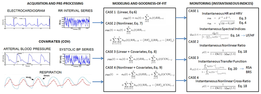
Figure 1. The flowchart of data acquisition and preprocessing (Phase I), modeling and goodness-of-fit assessment (Phase II), and monitoring (Phase III).

3. Methods and Data

3.1. Probability Models for the Heartbeat Interval

Given a set of R-wave events detected from the recorded ECG waveform, let RR_j = u_j − u_j−1 > 0 denote the jth R-R interval. By treating the R-waves as discrete events, we may develop a probabilistic point process model in the continuous-time domain. Assuming history dependence, the waiting time t − u_j (as a continuous random variable, where t > u_j) until the next R-wave event can be modeled by an inverse Gaussian model (Barbieri et al., 2005; Barbieri and Brown, 2006; Chen et al., 2009a)

where u_j denotes the previous R-wave event occurred before time t, þeta > 0 denotes the shape parameter (which might also be time-varying), and μ_RR(t) denotes the instantaneous R-R mean parameter. The use of an inverse Gaussian distribution to characterize the R-R intervals’ occurrences is further motivated by a physiological integrate-and-fire model of heartbeat generation: in fact, if the rise of the membrane potential to a threshold initiating the cardiac contraction is modeled as a Gaussian random-walk with drift, then the probability density of the times between threshold crossings (the R-R intervals) is indeed the inverse Gaussian distribution (Barbieri et al., 2005).

Note that when the mean μ_RR(t) is much greater than the variance, the inverse Gaussian distribution can be well approximated by a Gaussian distribution with an identical mean and a variance equal to . However, the inverse Gaussian distribution is more robust since it can better model the outliers due to its long tail behavior. In our earlier investigation (Chen et al., 2008, 2009a), we have compared heartbeat interval fitting point process models using different probability distributions, and found that the inverse Gaussian model achieved the overall best fitting results. In practice, we can always conduct an empirical model fit analysis (e.g., data histogram, the Q-Q plot, and the Kolmogorov-Smirnov plot) for the raw R-R intervals, testing the appropriateness of the inverse Gaussian model (Chen et al., 2011a).

In point process theory, the inter-event probability p(t) is related to the conditional intensity function (CIF) λ(t) by a one-to-one transformation (Brown et al., 2003)

The estimated CIF can be used to evaluate the goodness-of-fit of the probabilistic heartbeat interval model.

3.2. Instantaneous Indices of HR and HRV

Heart rate (HR) is defined as the reciprocal of the R-R intervals. For time t measured in seconds, the new variable r = c(t − u_j)⁻¹ (where c = 60 s/min is a constant) can be defined in beats per minute (bpm). By virtue of the change-of-variables formula, from equation (1) the HR probability p(r) = p(c(t − u_j)⁻¹) is given by p(r) = |dt/dr|p(t), and the mean and the SD of HR r can be derived (Barbieri et al., 2005)

where and . Essentially, the instantaneous indices of HR and HRV are characterized by the mean μ_HR and SD σ_HR, respectively. In a non-stationary environment, where the probability distribution of HR is possibly slowly changing over time, we aim to dynamically estimate the instantaneous mean μ_RR(t) and instantaneous shape parameter θ_t in equation (1) so that the evolution of the probability density p(r) can be tracked in an online fashion.

In Table 1, several potential probabilistic heartbeat interval models are listed, along with the derived probabilistic HR models (Chen et al., 2008, 2009a). For all probabilistic HR models, μ_HR and σ_HR can be either analytically derived or numerically evaluated. This provides a mathematically rigorous definition of instantaneous indices of HR and HRV, which sidesteps some of the difficulties in defining HR and HRV based on the series of heartbeat intervals unevenly distributed in time.

TABLE 1

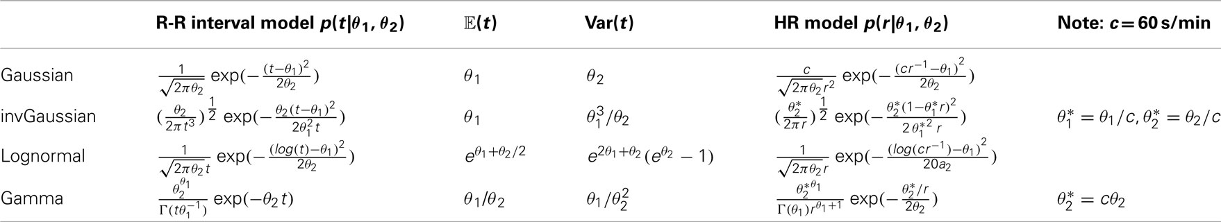
Table 1. List of four two-parameter parametric probabilistic models for the heartbeat R-R interval and heart rate (HR).

3.3. Autonomic Cardiovascular Control and Modeling Heartbeat Dynamics

In line with a control systems engineering approach, short term autonomic cardiovascular control can be modeled as a closed-loop system that involves blood pressure (BP) and respiratory (RP) measures as the two major variables that influence heartbeat dynamics (Baselli et al., 1988; De Boer et al., 1995; Barbieri et al., 2001). The closed-loop system can be illustrated by the simplified diagram shown in Figure 2. In the feedforward pathway (RR → BP), the R-R intervals influence the forthcoming BP measure as defined by the H₁₂ transfer function (either in the time or frequency domains), including the effects of heart contractility and vasculature tone on arterial pressure. In the feedback pathway (BP → RR), the autonomic nervous system modulates the beat-to-beat interval through a feedback control mechanism mediated by the baroreceptors, where the H₂₁ transfer function includes both baroreflex and autonomic control to the heart. In a second feedback pathway (RP → RR), the changes in lung volume modulates the beat-to-beat interval. The cardiovascular functions associated with these two feedback influences, baroreflex sensitivity (BRS) and respiratory sinus arrhythmia (RSA), operate within specific frequency bands.

FIGURE 2

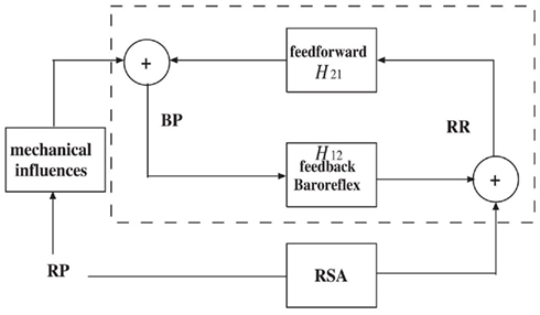
Figure 2. A simplified diagram of the cardiovascular closed-loop model. The beat-to-beat R-R interval is modulated by blood pressure (BP) through the feedback baroreflex loop. The dashed box represents a closed-loop baroreceptor-cardiac reflex (baroreflex) model. Outside the dashed box, the respiratory (RP) input also modulates RR through respiratory sinus arrhythmia (RSA) and modulates BP through mechanical influences.

A common methodological approach to characterize a physiological system is through system identification (Nikias and Petropulu, 1993; Marmarelis, 2004; Xiao et al., 2005). In general, let us consider a causal, continuous-time non-linear mapping F between an output variable y(t) and two input variables x(t) and u(t). Expanding the Wiener-Volterra series of function F (up to the second-order) with respect to inputs x(t) and u(t) yields (Schetzen, 1980)

where F(·): ℝ² ↦ ℝ is a non-linear function, and a(·), b(·), h₁(·,·), h₂(·,·), and h₃(·,·) are Volterra kernels with appropriate orders. In our cardiovascular system identification case, y(t) represents the expected heartbeat interval μ_RR(t), x(t) represents the previous R-R intervals, u(t) represents the vector of covariates (COV) such as BP or RP, and the continuous-time integral (convolution) is approximated by afinite and discrete summation. The first and second-order Volterra kernels will be replaced by discrete filter coefficients.

We consider four individual cases of discrete-time Volterra series expansion, which lead to different formulations to model the heartbeat interval mean μ_RR in equation (1).

• Dropping all of second-order terms as well as the COV terms in the Volterra series expansion (5), we obtain a univariate (noise-free) AR model

where the a₀ term is incorporated to compensate the non-zero mean of the R-R intervals.

• Dropping the COV terms in the Volterra series expansion (5), we obtain

where denotes the local mean of the past ℓ R-R intervals.

• Dropping all of second-order terms in the Volterra series expansion (5), we obtain a bivariate discrete-time linear system

where the first two terms represent a linear autoregressive (AR) model of the past R-R intervals, and COV_t−j denotes the previous jth covariate value prior to time t. Note that the COV observations will be preprocessed to have zero mean (since the DC component is of minimal importance to model the oscillation). Equation (8) can also be viewed as a linear (noise-free) autoregressive moving average (ARMA) model (Lu et al., 2001). Also note that here we have used RR_t−i instead of μ_RR(t − i) as regressors since this would require a higher order p due to the long-range dependence of μ_RR(t − i) under a very small timescale. Due to the absence of driving noise, Equation (8) can also be viewed as an ARX model, where the COV term serves as the exogenous input.

• Dropping the last two quadratic terms in the Volterra series expansion (5), we obtain

Equation (9) can be viewed as a bivariate bilinear system (Tsoulkas et al., 2001), which can also be viewed as a (noise-free) non-linear ARMA or non-linear ARX model (Lu et al., 2001).

3.4. Online Estimation: Adaptive Point Process Filtering and Local Likelihood Estimation

Since our earliest point process cardiovascular characterizations (Barbieri et al., 2005; Barbieri and Brown, 2006), in order to optimize the estimation of the model parameters, we have developed two model fitting algorithms: the adaptive point process filtering method (based on recursive adaptive filtering, and the local maximum likelihood (based on local likelihood estimation using a moving window). These two online estimation methods enable us to update the parameters of the heartbeat probability model at each moment in time in order to continuously track the non-stationary nature of the observations.

In the adaptive filtering method, let , denote the vector that contains all unknown parameters in the heartbeat interval probability model. Let the continuous-time interval be binned with a constant bin size Δ. A state-space formulation of the discrete-time (indexed by k) point process filtering algorithm is described here (Brown et al., 1998; Eden et al., 2004; Barbieri and Brown, 2006)

where P and W denote the parameter and noise covariance matrices, respectively; and Δ denotes the time bin size. The choice of bin size reflects the timescale of estimation interest, we typically use Δ = 5 ms. Diagonal noise covariance matrix W, which determines the level of parameter fluctuation at the timescale of Δ, can be either initialized empirically from the random-walk theory,¹ or estimated from the expectation-maximization (EM) algorithm (Smith and Brown, 2003). In our experiments, a typical value of noise variance value for the AR parameter is 10⁻⁶ ∼ 10⁻⁷, and the typical noise variance value for the shape parameter is 10⁻³ ∼ 10⁻⁴. The sensitivity analysis of the noise variance will be illustrated and discussed in the result section.

Symbols ▽λ_k = ∂λ_k/∂ξ_k and denote the first- and second-order partial derivatives of the CIF with respect to ξ at time t = kΔ, respectively. The indicator variable n_k = 1 if a heartbeat occurs in the time interval ((k − 1)Δ, kΔ] and 0 otherwise. The point process filtering equations can be viewed as a point process analog of the Kalman filtering equations in the presence of continuous-valued observations (Eden et al., 2004). Given a predicted (a priori) estimate ξ_k|k−1, the innovations [n_k − λ_kΔ] is weighted by P_k|k−1(▽logλ_k) (viewed as an adaptation gain) to further produce the filtered (a posteriori) estimate ξ_k|k. Since the innovations term is likely to be non-zero in the absence of a beat, the parameters are always updated at each time step k. The a posteriori error covariance P_k|k is derived based on a Gaussian approximation of the log-posterior (Eden et al., 2004). We always use the a posteriori estimate to the HR, HRV, and other statistics. The time-varying CIF λ_k is also numerically computed from equation (2) using the a posteriori estimate.

In the local likelihood estimation method (Loader, 1999), we can define the log-likelihood given an observation window (t − l, t] consisting of n heartbeat events {t − l < u₁ < u₂ < … < u_n ≤ t} as (Loader, 1999; Barbieri and Brown, 2006; Kodituwakku et al., 2012)

where (0 < α < 1) is a weighting function for the local likelihood estimation. The weighting time constant α governs the degree of influence of a previous event observation u_j on the local likelihood at time t. The second term of equation (10) represents the log-likelihood of the partially observed interval since the last observed beat u_n (right censoring). The local log-likelihood (10) can be optimized using a Newton-Raphson method to obtain a local maximum likelihood estimate of ξ (Loader, 1999).

The above estimation methods are by no means the only options. Other alternative methods can be considered. For instance, particle filtering is known to have a better tracking performance for non-linear dynamics at the cost of increasing memory and computational complexity (Brockwell et al., 2004; Ergun et al., 2007). In addition, instead of the Gaussian approximation, other types of approximation approaches may also be employed to obtain a more accurate point process filtering algorithm (Koyama et al., 2009, 2010).

3.5. Frequency Analysis

3.5.1. Estimating the frequency response at the feedback pathway (baroreflex or RSA)

Assuming a linear relation between the input and output of interest, we can estimate the transfer function (based on the Laplace transform) and the associated frequency response between the input and output variables (Saul et al., 1991; Pinna and Maestri, 2001; Xiao et al., 2005; Pinna, 2007).

In light of equation (8), the frequency response for the baroreflex (BP → RR) or RSA (RP → RR) is computed as (Chen et al., 2009a, 2011a)

where f₁ and f₂ denote the rate (beat/s) for the R-R and COV-COV intervals, respectively; here we assume f₁ ≈ f₂ ≡ f (we typically assume that the heartbeat period is about the same as the BP-event period, while the RP measurement can be resampled or interpolated at the beat time). The order of the AR model also determines the number of poles, or oscillations, in the frequency range. Modifying the AR coefficients is equivalent to changing the positions of the poles and reshaping the frequency response curve. With the time-varying AR coefficients {a_i(t)} and {b_j(t)} estimated from the point process filter, we can evaluate the dynamic frequency response of (11) at different ranges (LF, 0.04–0.15 Hz; HF, 0.15-min {0.5, 0.5/RR} Hz, where 0.5/RR denotes the Nyquist sampling frequency).

In the case where COV is BP, the frequency-dependent baroreflex gain or BRS, characterized by |H₁₂(f)|, represents the frequency-dependent modulation effect of BP on the heartbeat, mediated by the neural autonomic reflex. In the case where COV is RP, |H₁₂(f)| represents the frequency-dependent RSA gain.

3.5.2. Estimating the frequency response at the feedforward pathway

In the feedforward (RR → BP) pathway of Figure 2, the frequency response allows us to evaluate the impact of the heartbeat durations on the hemodynamics. In light of AR modeling in the feedback pathway, we can also model BP with a bivariate linear AR model

where μ_RR(k − i) represents the estimated instantaneous R-R mean value at the time bin when BP-events occur. The coefficients and are dynamically tracked by a RLS filter. Unlike the point process filter, the update occurs only at the occurrence time of BP-events, although it is important to highlight that the point process framework allows for these innovations to be associated with the evolution of the heartbeat dynamics at the exact time when the hemodynamic changes occur, without having to wait for the next heartbeat to be observed. Similarly, the frequency response of the RR → BP pathway can be estimated as

where f denotes the sampling rate (beat/s) for BP-BP intervals. Likewise, we can estimate the dynamic gain and phase of H₂₁(f) at each single BP-event (whereas during between-events period, the coefficient estimates remain unchanged).

3.5.3. Estimating the dynamic R-R spectrum

Let 𝒬_RR(f) denote the power spectrum of the R-R series. In the case of equation (6), 𝒬_RR(f) is estimated by

In the case of equation (8), 𝒬_RR(f) can be estimated by

From 𝒬_RR we can also compute the time-varying LF/HF power ratio. Note that we have assumed that the variance (estimated from the feedforward pathway) remains unchanged between two consecutive systolic BP values.

3.5.4. Estimating the dynamic coherence

In order to estimate the cross-spectrum in the context of a closed-loop system, we assume that the noise variance and the non-linear interactions in the feedforward and feedback loops are sufficiently small. From equation (11), we can estimate the cross-spectrum (between BP and RR) in the feedback loop as 𝒞_uy(f ) ≈ H₁₂(f )𝒬_BP(f). As the coefficients {a_i(t)} and {b_j(t)} are iteratively updated in time, the point process filter produces an instantaneous estimate of BRS as well as the cross-spectrum. Similarly, from equation (13) we can estimate the cross-spectrum in the feedforward pathway: 𝒞_yu(f) ≈ H₂₁(f)𝒬_RR(f).

Furthermore, the instantaneous normalized cross-spectrum (i.e., coherence) can be computed as

where |·| denotes the modulus of a complex variable. The second equality in equation (16) holds due to the fact that where *denotes the Hermitian operator (note that |𝒞_yu| = |𝒞_uy| and has anti-phase against each other). The third equality indicates that the time-varying coherence function can be expressed by the multiplication of two (feedback and feedforward) time-varying transfer functions (Zhao et al., 2005), computed from equations (11 and 13), respectively.

The time-varying closed-loop coherence function Coh(f, t) can be computed at very fine timescales by using two adaptive filters (i.e., the point process filter at the feedback pathway, and the RLS filter at the feedforward pathway) either synchronously or asynchronously, several studies have examined its properties (e.g., stability, numerical bound) in detail (Porta et al., 2002; Zhao et al., 2005, 2007).

3.6. Non-Linearity Assessment

Heartbeat dynamics are well known to be non-linear (Christini et al., 1995; Chon et al., 1996, 1997; Zhang et al., 2004; Chen et al., 2010a). In the literature, various non-linear indices such as the Lyapunov exponent, the fractal exponent, or the approximate entropy, have been proposed to characterize the non-linear behavior of the underlying physiological system (Peng et al., 1995; Ivanov et al., 1999; Akay, 2000; Teich et al., 2001; Costa et al., 2002; Struzik et al., 2004; Voss et al., 2009). It has been suggested that such non-linearity indices might provide informative indicators for diagnosing cardiovascular diseases (Poon and Merill, 1997; Goldberger et al., 2002; Tulppo et al., 2005; Atyabi et al., 2006).

Motivated by the importance of quantifying the contribution of non-linearity to HRV and the heartbeat dynamics, we have proposed a quantitative index based on the spectrum-bispectrum ratio (Chen et al., 2010a, 2011a)

The nominator of equation (17) corresponds to the R-R spectrum (or cross-spectrum between RR and COV in the presence of covariate), whereas the denominator corresponds to the sum of the R-R spectrum and R-R bispectrum (or cross-spectrum and cross-bispectrum in the presence of covariate). The above-defined ratio is frequency-dependent, and it is dimensionless and bounded between 0 and 1.

In both cases, the instantaneous ratio is derived as (see Chen et al., 2010a, 2011a) for assumptions and details)

where . The spectrum norm defines the area integrated over the frequency range under the spectral density curve. When the non-linear or bilinear interaction is small, the coefficients {h_kl} are small, and the ratio is close to 1.

3.7. Modeling Non-Stationary with the ARIMA Model

In time series modeling, it is common to “detrend” a time series by taking differences if the series exhibits undesired non-stationary features. The autoregressive integrated moving average (ARIMA) process may provide a suitable framework to achieve such a goal (Vu, 2007). Simply, the original time series is applied by a difference operator (one or more times) until the non-stationary trends are not observed in the ultimate series. This is essentially equivalent to applying a high-pass filter to get rid of the slow oscillation. Non-stationary trends are often observed in the epochs of experimental recordings of R-R intervals and/or other physiological measures, especially during the periods of intervention by external factors (e.g., drug administration, ventilation).

Motivated by this idea, we define the “increment of R-R series” {δRR_t−i} ≡ {RR_t−i − RR_t−i−1} and the “increment of COV series” {δCOV_t−i} ≡ {COV_t−i − COV_t−i−1}, and model the instantaneous heartbeat interval mean by the following new equation (Chen et al., 2010b)

The new series {δRR_t−i} and {δCOV_t−i} have zero mean and are combined within a new (noise-free) AR model in parallel with equation (8). Note that the a₀(t) term in equation (8) has been replaced by RR_t−1 in equation (19).

From equation (19), we can compute the differential frequency response between δRR and δCOV

When using BP as covariate, we call as the differential BRS; when using RP as covariate, is referred to as the differential RSA. Rearranging the terms {a_i(t)} and {b_j(t)} in equation (19) and applying the frequency analysis further yields the frequency response (in the conventional sense)

Note: It shall be pointed out that, due to the absence of the driven noise (equations 6–9, and 19), the terms AR, ARMA, ARX, or ARIMA models defined in this paper do not coincide with an AR-type model in the traditional sense. These models can be viewed as distinctive AR-type models with vanishing noise variance. In other words, as the uncertainty is embedded in the probability structure, we did not consider the noise component in modeling the mean.

3.8. Model Order Selection and Goodness-of-Fit Tests

Once a model is selected, we would need to predetermine the model order {p, q} of equations (6–9) in the selected Volterra series expansion. In general, the need of a tradeoff between model complexity and goodness-of-fit arises when a point process model is considered. In practice, the order of the model may be determined based on the Akaike information criterion (AIC; by pre-fitting a subset of the data using either the point process filter or the local likelihood method (Loader, 1999; Barbieri et al., 2005) as well as the Kolmogorov-Smirnov (KS) statistic (Brown et al., 2003) in the post hoc analysis. For different values p and q, we can compare the AIC and choose the parameter setup with the minimum AIC value. Let ℒ designate the log-likelihood value obtained from the pre-fitted data, the AIC is defined as

where dim(ξ) denotes the dimensionality of unknown parameter vector ξ used in the probability model of the heartbeat interval. In the presence of a non-linear or bilinear AR model, once the order is determined, the initial Volterra coefficients will be estimated by a least squares method (Westwick and Kearney, 2003). Specifically, the coefficients {a_i} are optimized by solving a Yule-Walker equation for the linear part using the first few hundreds sample points, and the coefficients {h_ij} are estimated by fitting the residual error via least squares. For the non-linear and bilinear models (equations 7 and 9), we use a sequential estimation instead of a joint estimation procedure for fitting the Volterra coefficients, since we prefer to preserve the interpretation of the linear AR coefficients. A joint estimation procedure is possible based on orthogonal projection, cross-correlation, or least squares (Marmarelis, 1993; Westwick and Kearney, 2003), although such method may destroy the structure described by the linear AR coefficients.

The goodness-of-fit of the point process model is based on the KS test (Brown et al., 2003). Given a point process specified by J discrete events: 0 < u₁ < … < u_J < T, the random variables are defined for j = 1, 2,…, J − 1. If the model is correct, then the variables v_j = 1 − exp(− z_j) are independent, uniformly distributed within the interval [0, 1], and the variables g_j = Φ⁻¹(v_j) (where Φ(·) denotes the cumulative distribution function (cdf) of the standard Gaussian distribution) are sampled from an independent standard Gaussian distribution. To conduct the KS test, the v_js are sorted from smallest to largest, and plotted against the cdf of the uniform density defined as (j − 0.5)/J. If the model is correct, the points should lie on the 45° line. The 95% confidence interval lines are defined as . The KS distance, defined as the maximum distance between the KS plot and the 45° line, is also used to measure lack-of-fit between the model and the data. The autocorrelation function of the g_js: , can also be computed. If the g_j s are independent, ACF(m) shall be small for any lag m, which is within the 95% confidence interval around 0.

3.9. Experimental Protocol and Data

A total of 15 healthy volunteer subjects (mean age 24 ± 4), gave written consent to participate in this study approved by the Massachusetts General Hospital (MGH) Department of Anesthesia and Critical Clinical Practices Committee, the MGH Human Research Committee and the MGH General Clinical Research Center. Subjects were evaluated with a detailed review of his/her medical history, physical examination, electrocardiogram, chest X-ray, a urine drug test, hearing test, and for female subjects, a pregnancy test. Any subject whose medical evaluation did not allow him or her to be classified as American Society of Anesthesiologists (ASA) Physical Status I was excluded from the study. Other exclusion criteria included neurological abnormalities, hearing impairment, and use of either prescribed or recreational psychoactive drugs. Intravenous and arterial lines were placed in each subject. Propofol was infused intravenously using a previously validated computer controlled delivery system running STANPUMP (a computer controlled delivery system; Shafer et al., 1988) connected to a Harvard 22 syringe pump (Harvard Apparatus, Holliston, MA), using the well-established pharmacokinetic and pharmacodynamic models (Schnider et al., 1998, 1999). In Subject 1, five effect-site target concentrations (0.0, 1.0, 2.0, 3.0, and 4.0 μg/ml) were each maintained for about 15 min respectively, where concentration level 0 corresponds to the conscious and wakefulness baseline. In the remainder of subjects, an additional effect-site target concentration of 5.0 μg/ml was administered. Capnography, pulse oximetry, ECG, and arterial blood pressure were monitored continuously by an anesthesiologist team throughout the study. Bag-mask ventilation with 30% oxygen was administered as needed in the event of propofol-induced apnea. Because propofol is a potent peripheral vasodilator, phenylephrine was administered intravenously to maintain mean arterial blood pressure (ABP) within 20% of the baseline value. ECG and ABP were recorded at a sampling rate of 1 kHz using a PowerLab ML795 data acquisition system (ADInstruments, Inc., Colorado Springs, CO). Four recordings (Subjects #6, 11, 12, 14) were excluded for analysis either because the subjects fell asleep during the experimental behavioral protocol or because of poor quality of the data recordings.

4. Results

Applications of the proposed point process framework to the experimental data led to instantaneous assessment of HRV, RSA, BRS, and of non-linearity of heartbeat dynamics in healthy subjects under progressive stages of propofol anesthesia (Chen et al., 2009b, 2010b, 2011a). All instantaneous indices are estimated to accommodate the non-stationary nature of the experimental recordings. Overall, our observations have revealed interesting dynamic trends across the experiment for individual subjects. Due to the tutorial nature of the current article, only three subjects (Subjects 5, 9, 15) are portrayed here for illustration purpose, detailed group comparison statistics can be found in (Chen et al., 2011a). The inverse Gaussian point process model for heartbeat intervals is considered in all the examples reported here, and all instantaneous indices are estimated using a point process filter with Δ = 5 ms temporal resolution.

4.1. Tracking Examples and Estimated Index Statistics

Figure 3 shows results from a subject (Subject 15) transitioning from level 0 to level 3 (several time intervals are replaced by shaded areas to appropriately portray all transitions of interest in one panel). In this subject, HRV, RSA, and BRS progressively decrease with increasing propofol administration, accompanied by a relevant increase in linear cardiorespiratory coupling as a result of dispensation of the first propofol bolus. Two sharp drops in BRS (within the LF range) are also observed at the level 0 → 1 and 1 → 2 transitions upon increasing the target drug concentration level. Meanwhile, RSA (within the HF range) also drops accordingly. Interestingly, the ratio ρ (computed with RP as COV) increases from level 0 to level 1 and then remains steady, suggesting that the non-linearity at the HF range slightly decreases with propofol administration. Table 2 shows a summary of the averaged statistics of the estimated instantaneous indices of interest within levels 1–3 as compared with baseline (level 0).

TABLE 2

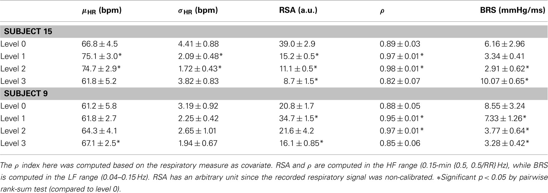
Table 2. Averaged statistics of the estimated instantaneous indices in the general anesthesia protocol (level 0–3 for two selected subjects).

FIGURE 3

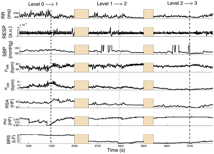
Figure 3. Tracking results of various instantaneous indices for Subject 15. Three transient periods (level 0 → 1, level 1 → 2, level 2 → 3) are shown (Chen et al. (2011b), Proceedings of EMBC. Reprinted with permission, Copyright © 2011 IEEE).

In a second example, Figure 4 shows a different subject (Subject 9) where, after the initial propofol administration, phenylephrine is administered to compensate a critical drop in blood pressure, followed by artificial ventilation. In this case, a sharp decrease in RSA is observed with anesthetic intervention, respiratory coupling is then partly restored, but systolic BP progressively decreases to critical levels, possibly due to baroreflex failure. After phenylephrine is administered (∼2960 s), BRS and systolic BP slightly recover, but fail to go back to baseline levels. During the period of apnea, artificial ventilation reflects in RSA variability and acts to restore HRV (as seen by the increase in σ_HR), only partly succeeding in raising BP levels via the feedforward pathway. Table 2 shows a summary of the averaged statistics of the estimated instantaneous indices for levels 1–3 as compared with the baseline (level 0), accompanied by a portrayal of the instantaneous dynamics observed within each level for the considered indices (Figure 5), confirming the progressive decrease in HRV, RSA, and BRS, as well as the linear cardiorespiratory coupling increase in the first two levels of propofol anesthesia.

FIGURE 4

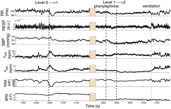
Figure 4. Tracking results of various instantaneous indices for Subject 9. The two dashed lines (∼2010 and ∼3000 s) mark the drug concentration level 0 → 1 (i.e., propofol administration onset time) and level 1 → 2, respectively. The dotted dashed line (∼2960 s) marks the time when phenylephrine was administered; and the dotted line (∼3125 s) marks the time of hand ventilation (Chen et al. (2011b), Proceedings of EMBC. Reprinted with permission, Copyright © 2011 IEEE).

FIGURE 5

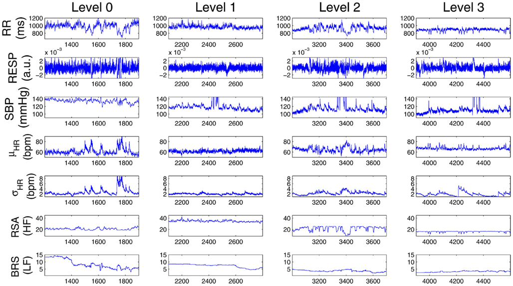
Figure 5. Comparison of the estimated instantaneous indices from four drug concentration levels (0–3) for Subject 9. Note that at each row, the vertical axes at all four panels have the same scale.

In addition, for pairwise comparison we also compute the mean statistic (averaged over time in each epoch) of all instantaneous indices during level 0 and level 1 drug concentrations for all 11 subjects. Figure 6 show the scatter plots for the mean HR, HRV, and BRS (LF range) values. More details can also be found in (Chen et al., 2011a).

FIGURE 6

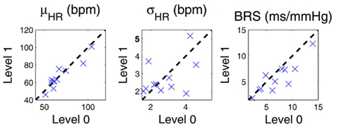
Figure 6. Scatter plots of the mean statistic (averaged over time in each epoch) of instantaneous HR, HRV, and BRS (LF range) indices during level 0 and level 1 drug concentrations for all 11 subjects. The dashed diagonal indicates a 45° line.

4.2. Example of Applying the ARIMA Model

Next, we illustrate how the use of ARIMA modeling (Section 3.7) can improve identification in the presence of highly non-stationary scenarios. The left panels of Figure 7 show the raw R-R interval series and systolic BP series are shown. In the considered subject (Subject 5), the systolic BP series has a decreasing trend (dropping from around 160–130 mmHg) within about 150 s, showing a high degree of non-stationarity (with a decreasing mean statistic along time). In contrast, the first-order difference series δRR and δSBP are stationary and have steady zero mean along time. As expected, modeling the mean heartbeat interval using equation (19) is more desirable than using equation (8). To verify our hypothesis, we have used the same model order (p = q = 8) for these two equations, and applied the point process model to fit the observed R-R and systolic BP series. The goodness-of-fit assessment shows that the ARIMA modeling improves the model fit with decreasing KS distance (from 0.0893 to 0.0513) in the KS test. Figure 8 shows the KS plot (including the KS statistic comparison) and the autocorrelation plot based on the ARIMA modeling. The fact that the curves fall within the 95% confidence intervals in both the KS and the autocorrelation plots indicates a good model description of the point process heartbeat events.

FIGURE 7

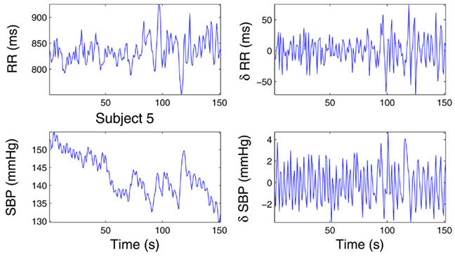
Figure 7. Experimental R-R interval series and systolic BP (SBP) series (left panels) from one recording epochs during level 1 propofol concentration. Their corresponding incremental series are also shown at the right panels. The raw SBP series has a decreasing trend (Chen et al. (2010b), Proceedings of EMBC. Reprinted with permission, Copyright © 2010 IEEE).

FIGURE 8

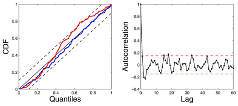
Figure 8. The estimated instantaneous indices from the data of Subject 5 (level 1 epoch) and the associated KS plot (left) and the autocorrelation plot (right). The KS statistic is improved from 0.0893 (standard model, red curve) to 0.0513 (ARIMA model, blue curve; Chen et al. (2010b), Proceedings of EMBC. Reprinted with permission, Copyright © 2010 IEEE).

4.3. Sensitivity Analysis

Finally, we perform sensitivity analysis to test the robustness of the proposed point process approach and the choice of parameters. Two issues are examined here. One is the choice of probability distribution (the inverse Gaussian against the Gaussian distribution) used for the R-R intervals. The other is the choice of the parameters used in the model and the point process filter.

To illustrate the first issue, we select the raw R-R intervals from one epoch at the level 0 drug concentration. Under the same point process framework, we fit the data with both the inverse Gaussian and Gaussian distributions for the inter-event intervals. Upon fitting the data, we compare their corresponding KS statistics. From the empirical data histogram (Figure 9A), it can be noticed that the distribution of the R-R intervals is asymmetric and slightly skewed (with a longer tail at the high value range). The Q-Q plot analysis also confirms that the inverse Gaussian distribution provides a better fit for the data (Figures 9C,D). As expected, the final KS statistic improves by using the inverse Gaussian (KS distance: 0.0562) rather than the Gaussian distribution (KS distance: 0.0719).In this case, although the fitted results from two models are very similar, only the inverse Gaussian model passes the KS test, i.e., its KS plot completely falls within the 95% confidence interval (Figure 9E).

FIGURE 9

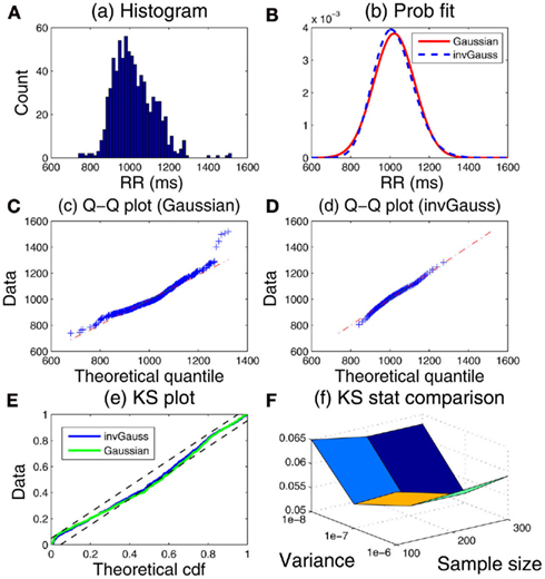
Figure 9. (A) Histogram of the R-R intervals from one selected epoch. (B) Maximum-likelihood-fitted Gaussian and inverse Gaussian distributions for the R-R intervals. (C,D) Q-Q plots for the Gaussian and inverse Gaussian distribution, respectively. (E) Comparative KS plots of point process model assessment using the inverse Gaussian and Gaussian distributions. (F) Comparison of KS statistics with different parameter initialization setups.

To illustrate the second issue of parameter estimation, the AR-type model parameters are initialized based on a subset of the same data used in Figure 9A at the start of the recordings. The data sample size used for initialization varies between 100, 200, and 300 (the time duration varies depending on the HR). The noise covariance matrix W in the filtering equation determines the level of parameter fluctuation at the every time step of Δ = 5 ms. For simplicity, we select different scale levels for the elements of W related to the AR parameters, on the order of 10⁻⁶, 10⁻⁷, and 10⁻⁸. Using the inverse Gaussian model, we compare the fitting KS statistic values under various parameter initialization setups and show the comparative result in Figure 9F. As seen, under a wide range of parameter choices, the fitted results are rather robust. The robustness of the performance can be ascribed to the flexibility of the random-walk model and to the fact that the tracking performance is insensitive to the exact value of the noise covariance matrix. Nevertheless, too large error covariance values will induce instability in the filtering operation, and cause unsatisfactory tracking performances. Finding an optimal range of the noise covariance matrix often involves a trial-and-error process based on a subset of the available recordings.

5. Discussion

Dynamic assessment of cardiovascular control is of fundamental importance to monitor physiological states that may change dramatically in very short time intervals. We have devised a unified point process probabilistic framework to assess heartbeat dynamics and autonomic cardiovascular control by using the heartbeat interval occurrences extracted from ECG recordings, together with other cardiovascular measures such as ABP and respiration. The proposed point process framework enables us to estimate instantaneous heartbeat dynamics (HR and HRV) as well as other cardiovascular functions (BRS and RSA) at fine temporal resolution. The Wiener-Volterra series expansion allows to model the instantaneous heartbeat interval based on the previously observed R-R intervals and selected cardiovascular covariates. The online estimation (adaptive point process filter or local likelihood method) allows us to track the fast transient dynamics of the indices. Currently, the model parameters are initialized based on small subset of recordings, and then allowed to be adapted based on an online estimation method. In the presence of high non-stationarity (e.g., baseline shift due to drugs or other effects), special attention is required in both modeling (such as using the ARIMA model) and parameter initialization (such as reinitializing the parameters based on observed informative markers).

Some limitations of our approach are worth mentioning. Currently, we are using the inverse Gaussian distribution for modeling the random heartbeat intervals. The inverse Gaussian distribution is a good candidate since it is more robust in modeling outliers due to its long-tailed behavior. However, just like many asymmetric long-tailed distributions (e.g., lognormal), the inverse Gaussian distribution can only capture outliers in the high value range (i.e., the long tail lies in the high percentile of the distribution). Therefore, it is insufficient to characterize potential outliers in the low-value range (i.e., outliers’ values smaller than the mean statistic). Another limitation of the current approach is that we have not separated the influences of blood pressure from that of respiration on HRV, which could produce some estimation bias for both BRS and RSA due to simplification of our model. How to integrate these physiological covariates all together still remains the subject of future investigation. One possibility is to consider a trivariate model. Another possibility is to incorporate a continuous-valued latent input that modulates μ_RR(t) within the point process model, and might account for the non-modeled physiological effect; in the maximum likelihood framework, for example, the latent variable can be inferred using an EM algorithm (Smith and Brown, 2003).

In applying the proposed point process framework to physiological data under a general anesthesia protocol, our outcomes have revealed important dynamics involved with procedures of induction of anesthesia. The study of transient periods due to pharmacological and physical intervention has demonstrated the capacity of the point process filter to quickly capture fast physiological changes within the cardiovascular system. For example, significant sudden variations in the instantaneous BRS in coincidence with interventional maneuvers suggests that baroreflex responses are supposedly triggered by sharp disturbances affecting the control system, whereas the clear reduction of BRS in correspondence to increasing induction of anesthesia might suggest that baroreflex responses are reset with propofol to control HR at a lower BP, and that BRS further decreases after administration as a result. The shift in the HR/BP set point may also reflect the propofol’s systemic vasodilatory effect, whereas baroreflex impairment is most likely the result of disruption of cardiac control within the central nervous system. The instantaneous indices associated with respiration further suggest that RSA gradually decreases from baseline after administration of propofol anesthesia, that RSA is generally suppressed by phenylephrine, and that the linear interactions within cardiorespiratory control remain stable or increase (Chen et al., 2009b). Specifically, RSA is likely to be mediated by withdrawal of vagal efferent activity resulting from either baroreflex response to spontaneous BP fluctuations, or respiratory gating of central arterial baroreceptor and chemoreceptor afferent inputs. From baseline to Level 1 we also observed an increase of non-linearity in the bilinear interactions between RR and systolic BP, accompanied by a significant decrease in linear coherence between these two series (Chen et al., 2011a). This seems to indicate that the non-linear component of the heartbeat dynamics during anesthesia is mainly generated from the cardiovascular (baroreflex) loop, with a more stable linear interaction maintained within cardiorespiratory coupling. It is also possible that the respiratory system indirectly influences HR by modulating the baroreceptor and chemoreceptor input to cardiac vagal neurons although, as in every cardiovascular system identification study, it is difficult to disentangle the separate influence of BP from the influence of respiration on HRV.

In light of these promising results, future directions of our research are aimed at further development and integration of a set of algorithms to preprocess the recorded signals prior to application of the modeling framework, to perform a robust and automated classification and correction of ECG-derived heartbeats, and to achieve an automatic determination procedure for tuning and initialization of the model parameters, with the final goal to devise a monitoring tool for real-time cardiovascular assessment.

Conclusion

In conclusion, we have appraised a comprehensive point process probabilistic framework to simultaneously assess linear and non-linear indices of HRV, together with important cardiovascular functions of interest. To date, the proposed point process framework has been successfully applied to a wide range of experimental protocols (Barbieri et al., 2005; Barbieri and Brown, 2006; Chen et al., 2009a, 2010a, 2011a; Kodituwakku et al., 2012). Although all of data analyses have been done in off-line laboratory settings, all of the developed statistical models pose a solid basis for devising a real-time quantitative tool to bestow vital indicators for ambulatory monitoring in clinical practice. Particularly in general anesthesia settings, the proposed instantaneous indices may provide a valuable quantitative assessment of the interaction between heartbeat dynamics and hemodynamics during general anesthesia, and they could be monitored intraoperatively in order to improve drug administration and reduce side-effects of anesthetic drugs.

Conflict of Interest Statement

The authors declare that the research was conducted in the absence of any commercial or financial relationships that could be construed as a potential conflict of interest.

Acknowledgments

The authors thank L. Citi, K. Habeeb, G. Harrell, R. Merhar, E. T. Pierce, A. Salazar, C. Tavares, and J. Walsh (Massachusetts General Hospital) for assistance with data collection and interpretation. Preliminary results of this article have been presented in Proc. IEEE EMBC’10, Buenos Aires, and Proc. IEEE EMBC’11, Boston, MA. The work was supported in part by NIH Grants R01-HL084502 (Riccardo Barbieri), DP1-OD003646 (Emery N. Brown), K25-NS05758 (Patrick L. Purdon), DP2-OD006454 (Patrick L. Purdon), as well as a CRC UL1 grant RR025758.

Footnote

1. ^According to the Gaussian random-walk theory, the variance or the translational squared distance of one random variable in one dimension within a time period is linearly proportional to the associated diagonal entry of W and the total time traveled.

References

Akay, M. (2000). Nonlinear Biomedical Signal Processing: Dynamic Analysis and Modeling, Vol. 2. New York: Wiley-IEEE Press.

Atyabi, F., Livari, M. A., Kaviani, K., and Tabar, M. R. R. (2006). Two statistical methods for resolving healthy individuals and those with congestive heart failure based on extended self-similarity and a recursive method. J. Biol. Phys. 32, 489–495.

Pubmed Abstract | Pubmed Full Text | CrossRef Full Text

Barbieri, R., and Brown, E. N. (2006). Analysis of heart beat dynamics by point process adaptive filtering. IEEE Trans. Biomed. Eng. 53, 4–12.

Pubmed Abstract | Pubmed Full Text | CrossRef Full Text

Barbieri, R., Matten, E. C., Alabi, A. A., and Brown, E. N. (2005). A point-process model of human heartbeat intervals: new definitions of heart rate and heart rate variability. Am. J. Physiol. Heart Circ. Physiol. 288, 424–435.

CrossRef Full Text

Barbieri, R., Parati, G., and Saul, J. P. (2001). Closed- versus open-loop assessment of heart rate baroreflex. IEEE Eng. Med. Biol. Mag. 20, 33–42.

Pubmed Abstract | Pubmed Full Text | CrossRef Full Text

Baselli, G., Cerutti, S., Civardi, S., Malliani, A., and Pagani, M. (1988). Cardiovascular variability signals: towards the identification of a closed-loop model of the neural control mechanisms. IEEE Trans. Biomed. Eng. 35, 1033–1046.

Pubmed Abstract | Pubmed Full Text | CrossRef Full Text

Berntson, G. G., Bigger, J. T., Eckberg, D. L., Grossman, P., Kaufmann, P. G., Malik, M., Nagaraja, H. N., Porges, S. W., Saul, J. P., Stone, P. H., and van der Molen, M. W. (1997). Heart rate variability: origins, methods, and interpretive caveats. Psychophysiology 34, 623–648.

Pubmed Abstract | Pubmed Full Text | CrossRef Full Text

Brockwell, A. E., Rojas, A., and Kass, R. E. (2004). Recursive Bayesian decoding of motor cortical signals by particle filtering. J. Neurophysiol. 91, 1899–1907.

Pubmed Abstract | Pubmed Full Text | CrossRef Full Text

Brown, E. N., Barbieri, R., Eden, U. T., and Frank, L. M. (2003). “Likelihood methods for neural data analysis,” in Computational Neuroscience: A Comprehensive Approach, ed. J. Feng (London: CRC Press), 253–286.

Brown, E. N., Frank, L. M., Tang, D., Quirk, M. C., and Wilson, M. A. (1998). A statistical paradigm for neural spike train decoding applied to position prediction from ensemble firing patterns of rat hippocampal place cells. J. Neurosci. 18, 7411–7425.

Pubmed Abstract | Pubmed Full Text

Chen, Z., Brown, E. N., and Barbieri, R. (2008). “A study of probabilistic models for characterizing human heart beat dynamics in autonomic blockade control,” in Proc. ICASSP’08, Las Vegas, NV, 481–484.

Chen, Z., Brown, E. N., and Barbieri, R. (2009a). Assessment of autonomic control and respiratory sinus arrhythmia using point process models of human heart beat dynamics. IEEE Trans. Biomed. Eng. 56, 1791–1802.

CrossRef Full Text

Chen, Z., Purdon, P. L., Pierce, E. T., Harrell, G., Walsh, J., Salazar, A. F., Tavares, C. L., Brown, E. N., and Barbieri, R. (2009b). “Linear and nonlinear quantification of respiratory sinus arrhythmia during propofol general anesthesia,” in Proceedings of IEEE 31st Annual Conference Engineering in Medicine and Biology (EMBC’09), Minneapolis, MN, 5336–5339.

Chen, Z., Brown, E. N., and Barbieri, R. (2010a). Characterizing nonlinear heartbeat dynamics within a point process framework. IEEE Trans. Biomed. Eng. 57, 1335–1347.

CrossRef Full Text

Chen, Z., Purdon, P. L., Brown, E. N., and Barbieri, R. (2010b). “A differential autoregressive modeling approach within a point process framework for non-stationary heartbeat intervals analysis,” in Proceedings of IEEE 32nd Annual Conference Engineering in Medicine and Biology (EMBC’10), Buenos Aires, 3567–3570.

Chen, Z., Purdon, P. L., Pierce, E. T., Harrell, G., Walsh, J., Brown, E. N., and Barbieri, R. (2011a). Dynamic assessment of baroreflex control of heart rate during induction of propofol anesthesia using a point process method. Ann. Biomed. Eng. 39, 260–276.

CrossRef Full Text

Chen, Z., Citi, L., Purdon, P. L., Brown, E. N., and Barbieri, R. (2011b). “Instantaneous assessment of autonomic cardiovascular control during general anesthesia,” in Proceedings of IEEE 33rd Annual Conference Engineering in Medicine and Biology (EMBC’11), Boston, MA, 8444–8447.

Chon, K. H., Mukkamala, R., Toska, K., Mullen, T. J., Armoundas, A. A., and Cohen, R. J. (1997). Linear and nonlinear system identification of autonomic heart-rate modulation. IEEE Eng. Med. Biol. Mag. 16, 96–105.

Pubmed Abstract | Pubmed Full Text | CrossRef Full Text

Chon, K. H., Mullen, T. J., and Cohen, R. J. (1996). A dual-input nonlinear system analysis of autonomic modulation of heart rate. IEEE Trans. Biomed. Eng. 43, 530–540.

Pubmed Abstract | Pubmed Full Text | CrossRef Full Text

Christini, D. J., Bennett, F. M., Lutchen, K. R., Ahmed, H. M., Hausdofi, J. M., and Oriol, N. (1995). Application of linear and nonlinear time series modeling to heart rate dynamics analysis. IEEE Trans. Biomed. Eng. 42, 411–415.

Pubmed Abstract | Pubmed Full Text | CrossRef Full Text

Costa, M., Goldberger, A. L., and Peng, C.-K. (2002). Multiscale entropy analysis of complex physiologic time series. Phys. Rev. Lett. 89, 068102.

Pubmed Abstract | Pubmed Full Text | CrossRef Full Text

Daley, D. J., and Vere-Jones, D. (2007). An Introduction to the Theory of Point Processes, Vol. 1, 2. New York: Springer.

De Boer, R. W., Karemaker, J. M., and Strackee, J. (1995). Relationships between short-term blood-pressure fluctuations and heart-rate variability in resting subjects: a spectral analysis approach. Med. Biol. Eng. Comput. 23, 352–358.

CrossRef Full Text

Eckberg, D. L. (2008). Arterial baroreflexes and cardiovascular modeling. Cardiovasc. Eng. 8, 5–13.

Pubmed Abstract | Pubmed Full Text | CrossRef Full Text

Eden, U. T., Frank, L. M., Solo, V., and Brown, E. N. (2004). Dynamic analyses of neural encoding by point process adaptive filtering. Neural Comput. 16, 971–998.

Pubmed Abstract | Pubmed Full Text | CrossRef Full Text

Ergun, A., Barbieri, R., Eden, U. T., Wilson, M. A., and Brown, E. N. (2007). Construction of point process adaptive filter algorithms for neural systems using sequential Monte Carlo methods. IEEE Trans. Biomed. Eng. 54, 419–428.

Pubmed Abstract | Pubmed Full Text | CrossRef Full Text

Goldberger, A. L., Peng, C.-K., and Lipsitz, L. A. (2002). What is physiologic complexity and how does it change with aging and disease? Neurobiol. Aging 23, 23–26.

Pubmed Abstract | Pubmed Full Text | CrossRef Full Text

Haykin, S. (2001). Adaptive Filter Theory, 4th Edn. Upper Saddle River, NJ: Prentice Hall.

Ivanov, P. C., Amaral, L. A., Goldberger, A. L., Havlin, S., Rosenblum, M. G., Struzik, Z. R., and Stanley, H. E. (1999). Multifractality in human heartbeat dynamics. Nature 399, 461–465.

Pubmed Abstract | Pubmed Full Text | CrossRef Full Text

Jo, J. A., Blasi, A., Valladares, E. M., Juarez, R., Baydur, A., and Khoo, M. C. K. (2007). A nonlinear model of cardiac autonomic control in obstructive sleep apnea syndrome. Ann. Biomed. Eng. 35, 1425–1443.

Pubmed Abstract | Pubmed Full Text | CrossRef Full Text

Khoo, M. C. K. (1999). Physiological Control Systems: Analysis, Simulation, and Estimation. New York: Wiley-IEEE Press.

Kodituwakku, S., Lazar, S. W., Indic, P., Chen, Z., Brown, E. N., and Barbieri, R. (2012). Point process time-frequency analysis of dynamic breathing patterns during meditation practice. Med. Biol. Eng. Comput. (in press).

Korenberg, M. J. (1991). Parallel cascade identification and kernel estimation for nonlinear systems. Ann. Biomed. Eng. 19, 429–455.

Pubmed Abstract | Pubmed Full Text | CrossRef Full Text

Koyama, S., Castellanos Pérez-Bolde, L., Shalizi, C. R., and Kass, R. E. (2010). Approximate methods for state-space models. J. Am. Stat. Assoc. 105, 170–180.

Pubmed Abstract | Pubmed Full Text | CrossRef Full Text

Koyama, S., Eden, U. T., Brown, E. N., and Kass, R. E. (2009). Bayesian decoding of neural spike trains. Ann. Inst. Stat. Math. 62, 37–59.

CrossRef Full Text

Loader, C. (1999). Local Regression and Likelihood. New York: Springer.

Lu, S., Ju, K. H., and Chon, K. H. (2001). A new algorithm for linear and nonlinear ARMA model parameter estimation using affine geometry. IEEE Trans. Biomed. Eng. 48, 1116–1124.

Pubmed Abstract | Pubmed Full Text | CrossRef Full Text

Marmarelis, P. Z. (1993). Identification of nonlinear biological systems using Laguerre expansions of kernels. Ann. Biomed. Eng. 21, 573–589.

Pubmed Abstract | Pubmed Full Text | CrossRef Full Text

Marmarelis, V. Z. (2004). Nonlinear Dynamic Modeling of Physiological Systems. New York: Wiley.

Nikias, C., and Petropulu, A. P. (1993). Higher Order Spectra Analysis: A Non-Linear Signal Processing Framework. Englewood Cliffs, NJ: Prentice Hall.

Parati, G., DiRienzo, M., and Mancia, G. (2001). Dynamic modulation of baroreflex sensitivity in health and disease. Ann. N. Y. Acad. Sci. 940, 469–487.

Pubmed Abstract | Pubmed Full Text | CrossRef Full Text

Peng, C. K., Havlin, S., Stanley, H. E., and Goldberger, A. L. (1995). Quantification of scaling exponents and crossover phenomena in nonstationary heartbeat time series. Chaos 5, 82–87.

Pubmed Abstract | Pubmed Full Text | CrossRef Full Text

Pinna, G. D. (2007). Assessing baroreflex sensitivity by the transfer function method: what are we really measuring? J. Appl. Physiol. 102, 1310–1311.

Pubmed Abstract | Pubmed Full Text | CrossRef Full Text

Pinna, G. D., and Maestri, R. (2001). New criteria for estimating baroreflex sensitivity using the transfer function method. J. Med. Biol. Eng. Comput. 40, 79–84.

CrossRef Full Text

Poon, C.-S., and Merill, C. K. (1997). Decrease of cardiac chaos in congestive heart failure. Nature 389, 492–495.

Pubmed Abstract | Pubmed Full Text | CrossRef Full Text

Porta, A., Aletti, F., Vallais, F., and Baselli, G. (2009). Multimodal signal processing for the analysis of cardiovascular variability. Philos. Trans. R. Soc. Lond. A 367, 391–409.

CrossRef Full Text

Porta, A., Furlan, R., Rimoldi, O., Pagani, M., Malliani, A., and van de Borne, P. (2002). Quantifying the strength of linear causal coupling in closed loop interacting cardiovascular variability signals. Biol. Cybern. 86, 241–251.

Pubmed Abstract | Pubmed Full Text | CrossRef Full Text

Purdon, P. L., Pierce, E. T., Bonmassar, G., Walsh, J., Harrell, P. G., Kwo, J., Deschler, D., Barlow, M., Merhar, R. C., Lamus, C., Mullaly, C. M., Sullivan, M., Maginnis, S., Skoniecki, D., Higgins, H. A., and Brown, E. N. (2009). Simultaneous electroencephalography and functional magnetic resonance imaging of general anesthesia. Ann. N. Y. Acad. Sci. 1157, 61–70.

Pubmed Abstract | Pubmed Full Text | CrossRef Full Text

Ross, S. M. (1997). Introduction to Probability Models, 6th Edn. San Diego, CA: Academic Press.

Saul, J. P., Berger, R. D., Albrecht, P., Stein, S. P., Chen, M. H., and Cohen, R. J. (1991). Transfer function analysis of the circulation: unique insights into cardiovascular regulation. Am. J. Physiol. Heart Circ. Physiol. 261, H1231–H1245.

Saul, J. P., and Cohen, R. J. (1994). “Respiratory sinus arrhythmia,” in Vagal Control of the Heart: Experimental Basis and Clinical Implications, eds M. N. Levy, and P. J. Schwartz (Armonk, NY: Futura Publishing Inc.), 511–536.

Schetzen, M. (1980). The Volterra and Wiener Theories of Nonlinear Systems. New York: Wiley.

Schnider, T. W., Minto, C. F., Gambus, P. L., Andresen, C., Goodale, D. B., Shafer, S. L., and Youngs, E. J. (1998). The influence of method of administration and covariates on the pharmacokinetics of propofol in adult volunteers. Anesthesiology 88, 1170–1182.

Pubmed Abstract | Pubmed Full Text | CrossRef Full Text

Schnider, T. W., Minto, C. F., Shafer, S. L., Gambus, P. L., Andresen, C., Goodale, D. B., and Youngs, E. J. (1999). The influence of age on propofol pharmacodynamics. Anesthesiology 90, 67–72.

CrossRef Full Text

Shafer, A., Doze, V. A., Shafer, S. L., and White, P. F. (1988). Pharmacokinetics and pharmacodynamics of propofol infusions during general anesthesia. Anesthesiology 69, 348–356.

Pubmed Abstract | Pubmed Full Text | CrossRef Full Text

Smith, A. C., and Brown, E. N. (2003). Estimating a state-space model from point process observations. Neural Comput. 15, 965–991.

Pubmed Abstract | Pubmed Full Text | CrossRef Full Text

Stauss, H. M. (2003). Heart rate variability. Am. J. Physiol. Regul. Integr. Comp. Physiol. 285, R927–R931.

Pubmed Abstract | Pubmed Full Text

Struzik, Z. R., Hayano, J., Sakata, S., Kwak, S., and Yamamoto, Y. (2004). 1/f scaling in heart rate requires antagonistic autonomic control. Phys. Rev. E Stat. Nonlin. Soft Matter Phys. 70, 050901.

Pubmed Abstract | Pubmed Full Text | CrossRef Full Text

Task Force. (1996). Task Force of the European Society of Cardiology, and the North American Society of Pacing, and Electrophysiology. Heart rate variability. Circulation 93, 1043–1065.

Pubmed Abstract | Pubmed Full Text | CrossRef Full Text

Teich, M. C., Lowen, S. B., Jost, B. M., Vibe-Rheymer, K., and Heneghan, C. (2001). “Heart rate variability: measures and models,” in Nonlinear Biomedical Signal Processing, Vol. 2, Dynamic Analysis and Modeling, ed. M. Akay (New York: Wiley-IEEE), 159–212.

Tsoulkas, V., Koukoulas, P., and Kalouptsidis, N. (2001). Identification of input output bilinear systems using cumulants. IEEE Trans. Signal Process. 49, 2753–2761.

CrossRef Full Text

Tulppo, M. P., Kiviniemi, A. M., Hautala, A. J., Kallio, M., Seppanen, T., Makikallio, T. H., and Huikuri, H. V. (2005). Physiological background of the loss of fractal heart rate dynamics. Circulation 112, 314–319.

Pubmed Abstract | Pubmed Full Text | CrossRef Full Text

Voss, A., Schulz, S., Schroeder, R., Baumert, M., and Caminal, P. (2009). Methods derived from nonlinear dynamics for analysing heart rate variability. Philos. Trans. R. Soc. Lond. A 367, 277–296.

CrossRef Full Text

Vu, K. M. (2007). The ARIMA and VARIMA Time Series: Their Modelings, Analyses and Applications. AuLac Technologies, Inc. Available at: http://www.chegg.com/textbooks/arima-and-varima-time-series-their-modelings-analyses-and-applications-1st-edition-9780978399610-0978399617

Wang, H., Ju, K., and Chon, K. H. (2007). Closed-loop nonlinear system identification via the vector optimal parameter search algorithm: application to heart rate baroreflex control. Med. Eng. Phys. 29, 505–515.

Pubmed Abstract | Pubmed Full Text | CrossRef Full Text

Westwick, D. T., and Kearney, R. E. (2003). “Explicit least-squares methods,” in Identification of Nonlinear Physiological Systems, Chap. 7 (New York: Wiley), 169–206.

Xiao, X., Mullen, T. J., and Mukkamala, R. (2005). System identification: a multi-signal approach for probing neural cardiovascular regulation. Physiol. Meas. 26, R41–R71.

Pubmed Abstract | Pubmed Full Text | CrossRef Full Text

Zhang, Y., Wang, H., Ju, K. H., Jan, K.-M., and Chon, K. H. (2004). Nonlinear analysis of separate contributions of autonomous nervous systems to heart rate variability using principal dynamic modes. IEEE Trans. Biomed. Eng. 26, 255–262.

CrossRef Full Text

Zhao, H., Cupples, W. A., Ju, K., and Chon, K. H. (2007). Time-varying causal coherence function and its application to renal blood pressure and blood flow data. IEEE Trans. Biomed. Eng. 54, 2142–2150.

Pubmed Abstract | Pubmed Full Text | CrossRef Full Text

Zhao, H., Lu, S., Zou, R., Ju, K., and Chon, K. H. (2005). Estimation of time-varying coherence function using time-varying transfer functions. Ann. Biomed. Eng. 33, 1582–1594.

Pubmed Abstract | Pubmed Full Text | CrossRef Full Text

Zou, R., Wang, H., and Chon, K. H. (2003). A robust time-varying identification algorithm using basis functions. Ann. Biomed. Eng. 31, 840–853.

Pubmed Abstract | Pubmed Full Text | CrossRef Full Text