
- Department of Ophthalmology, Schepens Eye Research Institute, Harvard Medical School, Boston, MA, USA
Perceived blur is an important measure of image quality and clinical visual function. The magnitude of image blur varies across space and time under natural viewing conditions owing to changes in pupil size and accommodation. Blur is frequently studied in the laboratory with a variety of digital filters, without comparing how the choice of filter affects blur perception. We examine the perception of image blur in synthetic images composed of contours whose orientation and curvature spatial properties matched those of natural images but whose blur could be directly controlled. The images were blurred by manipulating the slope of the amplitude spectrum, Gaussian low-pass filtering or filtering with a Sinc function, which, unlike slope or Gaussian filtering, introduces periodic phase reversals similar to those in optically blurred images. For slope-filtered images, blur discrimination thresholds for over-sharpened images were extremely high and perceived blur could not be matched with either Gaussian or Sinc filtered images, suggesting that directly manipulating image slope does not simulate the perception of blur. For Gaussian- and Sinc-blurred images, blur discrimination thresholds were dipper-shaped and were well-fit with a simple variance discrimination model and with a contrast detection threshold model, but the latter required different contrast sensitivity functions for different types of blur. Blur matches between Gaussian- and Sinc-blurred images were used to test several models of blur perception and were in good agreement with models based on luminance slope, but not with spatial frequency based models. Collectively, these results show that the relative phases of image components, in addition to their relative amplitudes, determines perceived blur.
Introduction
Blur is a fundamental image property; it is an important dimension in image quality assessment and in the clinic, blur is implicated in eye growth and development of myopia and hyperopia (Wallman et al., 1978; Hodos and Kuenzel, 1984) and it is critical for satisfaction with optical correction (Ciuffreda et al., 2006; Woods et al., 2010). For synthetic edge-based images, the estimation of image blur has been studied in some detail and many edge-finding and image processing models explicitly represent blur (see Morgan and Watt, 1997 for review). For example, the perceived blur of the edges in an image could depend on the gradient at the zero crossings (Marr and Hildreth, 1980), on the separation between peaks in either the second derivative of luminance (Watt and Morgan, 1983) or in the summed outputs of a bank of band-pass filters (Watt and Morgan, 1985), the scale of cascaded filters producing peak response to a blurred edge (Georgeson et al., 2007), the slope of the amplitude spectrum of the image (Tolhurst and Tadmor, 1997), or the relative contrast at high spatial frequencies (Mather, 1997).
Many previous studies have employed different methods to simulate image blur, including, but not limited to, square, cosine and Gaussian profile edges (Watt and Morgan, 1985) and manipulations of the slope of the amplitude spectrum in complex images (Webster et al., 2002), but there have been few efforts to compare perceived blur or model fits for different blur methods. In this study, we compare blur in images that were filtered with three commonly applied digital image processing methods:
(1) Slope of the Amplitude Spectrum.
The amplitude spectrum of natural images is inversely related to spatial frequency (Field, 1987), with a slope that falls between −0.7 and −1.5 on log–log axes (Burton and Moorhead, 1987; Billock et al., 2001). This so-called 1/F scaling originates from the fact that illumination and object surface properties are highly correlated over short distances (Ruderman, 1997), which in turn give rise to the presence of edges where boundaries and occlusions occur. The logarithmic bandwidths and spacing of filters in the human visual system produces a population response to natural images that is approximately constant across spatial scales (Field, 1987). This has lead to the suggestion that image blur might be estimated from the relative energy at high spatial frequencies (Marr and Hildreth, 1980; Mather, 1997) or, equivalently, the slope of the amplitude spectrum (Brady et al., 1997; Tolhurst and Tadmor, 1997). The slope of the amplitude spectrum is frequently manipulated to study perceived blur and blur adaptation (Webster et al., 2002; Vera-Diaz et al., 2010). One advantage of this method is that it allows the generation of images with a slope that is shallower or steeper than the original image and these departures are respectively referred to as “sharper” or “blurrier” than the original. Figure 1A illustrates the change in appearance of a contoured image as the slope varies linearly from −0.5 at the top to −3 at the bottom. It remains unclear whether over-sharp images (e.g., top of Figure 1A) actually appear less blurred than a sharp image. Given the improbability of an over-sharp stimulus appearing in the natural environment, it is unknown how such an unfocused profile is perceived qualitatively.
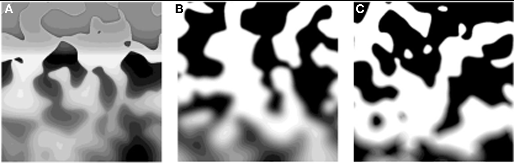
Figure 1. Illustrations of representative stimuli, drawn to scale. Images with smoothly varying, sharp contours were generated from binarized, low-pass filtered, 512 × 512 pixel noise images. Blur was manipulated by (A) varying the slope of the amplitude spectrum linearly from −0.5 at the top to −3 at the bottom; (B) blurring with a Gaussian with σ standard deviation from 64 to 2 cpi; (C) blurring with a Sinc function with λ varying from 256 to 8 cpi (see text and Figure 2 for details).
(2) Gaussian Low-Pass Filtering.
Gaussian blurring is frequently employed to represent image blurring caused by statistical light scatter and sampling by receptive fields with Gaussian profiles. In the clinic, Gaussian blurring is responsible for decreased acuity in the presence of cataracts. In computational modeling and digital image processing, by far the most widely used method of image blurring is through Gaussian low-pass filtering (for review see Gonzalez et al., 2004), illustrated in Figure 1B. Like manipulations of image slope, Gaussian blurring changes the amplitude, but not the phase of different image components.
(3) Aperture Blur.
The modulation transfer function of an optical system is partially determined by the diameter of its aperture, which for the eye is the pupil. The diameter of the pupil is constantly changing, but we are not usually aware of changes in perceived blur. Such pupil blur can be calculated by taking the amplitude spectrum of the aperture and for a circular aperture, it corresponds to a Sinc function that introduces phase reversals as well as attenuation of high spatial frequency components. Figure 1C illustrates the effects of aperture blur.
By swapping amplitude and phase spectra of different images, many studies have demonstrated that the appearance of an image is determined by both its amplitude and its phase spectrum (Oppenheim and Lim, 1981; Piotrowski and Campbell, 1982; Morgan et al., 1991; Tadmor and Tolhurst, 1993; Thomson et al., 2000; Bex and Makous, 2002). In this manuscript, we examine how perceived blur is affected by the phase reversals that are introduced by aperture blur, but not by slope or Gaussian blur. We aimed to compare the perception of blur generated by different digital image processing methods in images of natural scenes. However, the limited depth of focus in available calibrated natural images means that some parts of any image might be in focus, while others might be out of focus by an unknown quantity. Moreover, there is no available ground truth for calculating the actual level of blur or object distance in these images because differences in focal point and scene properties give rise to large and unknown variation in amplitude spectrum across the image. Therefore these natural images are unsuitable for the study of overall perceived image blur. We instead generated synthetic images that share many of the properties of natural images, but whose blur could be precisely specified. We used binarized filtered noise images because they have the same mean amplitude spectra of natural images. In the Appendix, we include a series of computations showing that the orientation and curvature structure of the contours present in these synthetic stimuli closely resemble those found in images of natural scenes (Geisler et al., 2001), except that the blur in these images can be directly specified. The use of a new pair of random noise image each trial ensured that each image was unique and this helped to avoid the buildup of local adaptation effects (Webster et al., 2002) or point-wise comparisons between stimulus pairs. The synthetic images were generated by low-pass filtering a new random noise image each trial and then assigning each pixel a binary value according to whether the pixel was above or below the mean. Example stimuli are shown in Figure 1. In order to examine the perception of blur in these images, in Experiment 1 observers discriminated images that were blurred to different levels with the same method. In Experiment 2, observers matched the apparent blur between image pairs that were filtered with different methods.
Materials and Methods
Subjects
The authors and four volunteers who were naïve to the hypotheses of the experiment served as observers. Their mean age was 25 years (σ 10 years) and all had normal or corrected to normal vision. All subjects completed practice trials before formal data collection to familiarize themselves with the manipulation of blur in the present images. The experimental procedures conformed to the tenets of the declaration of Helsinki and were approved by the departmental Institutional Review Board.
Stimuli
Stimuli were generated on a PC computer using MatLab™ software and employed routines from the Psychophysics Toolbox (Brainard, 1997; Pelli, 1997). Stimuli were displayed with a GeForce4 MX440 graphics card driving a Sony Trinitron Multiscan 200ES monitor with a mean luminance of 50 cd/m2 and a frame rate of 60 Hz. The display measured 36° horizontally (1152 pixels), 27° vertically (870 pixels), and was positioned 57 cm from the observer in an otherwise dark room. The luminance gamma functions for red, green, and blue were measured separately with a Minolta LS110 photometer and were corrected directly in the graphics card’s control panel to produce linear 8 bit resolution per color. The monitor settings were adjusted so that the luminance of green was twice that of red, which in turn was twice that of blue. This shifted the white-point of the monitor to 0.31, 0.28 (x,y) at 50 cd/m2. A bit-stealing algorithm (Tyler, 1997) was used to obtain 10.8 bits (1785 unique levels) of luminance resolution under the constraint that no RGB value could differ from the others by more than one look up table step.
Naturally contoured stimuli were generated from filtered noise images. Each trial, a pair of new standard and reference random noise images, each 512 × 512 pixels, was low-pass filtered in the Fourier domain with a Gaussian (Eq. 1) with a standard deviation of four cycles per image (4°) and zero DC. Standard and reference images were different from each other to prevent observers from comparing the same feature(s) in each image. A threshold was applied to the filtered image, such that pixels below the mean value (0) were assigned −1 and pixels above the mean assigned +1. This process produced unique images containing many smoothly curved contours that were in sharp focus at all points in the image. The slope of the amplitude spectrum was measured for 1000 such images and was −1.24 (σ = 0.03), which is close to the typical “1/F” slope of the amplitude spectrum of natural images (Burton and Moorhead, 1987; Billock et al., 2001). The amplitude spectrum was computed using the fft2() function in Matlab for a new 512 square random noise image that was zero padded to 1024 × 1024 pixels and truncated with a circular Tukey window (Ramirez, 1985). The amplitude was summed across all orientations within abrupt one-octave bands centered at 1–256 cycles per image in nine log spaced steps. Log amplitude versus log frequency was fit with linear regression to determine the “1/F’ slope for each image. Examples of typical images are shown in Figure 1.
Three classes of image blur were studied:
(1) Slope – the slope of the amplitude spectrum of the image was fixed at the required value. This process allowed for slopes that were “sharper” than the original image, i.e., slopes that were shallower than the original (−1.24) were more sharp than the source image, while slopes that were steeper than the original were more blurred than the source image. Figure 1A shows a scale image in which the slope decreases linearly from −0.5 at the top of the image, to −3 at the bottom.
(2) Gaussian low-pass filters were defined in the Fourier domain as:
where ω is spatial frequency and σ specifies the Gaussian standard deviation. Figure 1B shows a scale image in which σ decreases logarithmically from 64 cycles per image at the top of the image, to two cycles per image at the bottom.
(3) Sinc filters were defined in the Fourier domain as:
where λ determines the spatial frequency (ω) at which phase first reverses (see Figure 4 for profiles of this filter). Figure 1C shows a scale image in which λ decreases logarithmically from 64 cycles per image at the top of the image, to two cycles per image at the bottom.
Experiment 1 Blur Discrimination Thresholds
A standard and a test image were generated from each source image. The blur level of the standard was as follows: for slope-blurred images, the slope of the amplitude spectrum was fixed at −0.5, −1, −1.5, −2, −2.5, −3; For Gaussian-blurred images, σ was fixed at 0.25, 0.5, 1, 2, 4, 8, 16, 32 c/degree (2–256 cycles per image); for Sinc-blurred images, λ was fixed at 1, 2, 4, 8, 16, 32, 64 c/degree (8–512 cycles per image). The blur level of the test image was under the control of a three-down-one-up staircase (Wetherill and Levitt, 1965) designed to converge at a contrast increment producing 79.4% correct responses. The staircases were initialized with random start values within ±4 dB of a 20% Weber threshold estimated in pilot runs; the step size was initially 2 dB and was reduced to 1 dB after two reversals. The standard and test images were independently assigned a RMS contrast randomly drawn from a normal distribution with a mean of 0.3 and a standard deviation of 0.1. This randomization of contrast ensured that observers could not reliably base their blur estimates on image contrast, which is known to affect perceived blur (Watt and Morgan, 1983).
The standard and test images were presented for 1 s in a 16° circular window, centered 8° to the left or right of fixation, at random across trials. The edge of the window was smoothed with a raised cosine over 0.25° (8 pixels) and the onset and offset of the stimuli was smoothed with a raised cosine over 40 ms (three video frames). The observer’s 2AFC task was to identify whether the more blurred image (test) was on the left or right of fixation. Visual feedback was provided at the fixation mark, which was 50 cd/m2 (like the background) green following a correct response, or 50 cd/m2 red following an incorrect response, and was present at all times throughout the experiment.
The raw data from a minimum of four runs for each condition (at least 160 trials per psychometric function) were combined and fit with a cumulative normal function by minimization of chi-square (in which the percent correct at each test contrast were weighted by the binomial standard deviation based on the number of trials presented at that contrast). Blur discrimination thresholds were estimated from the 75% correct point of the best-fitting psychometric function. 95% confidence intervals on this point were calculated with a bootstrap procedure, based on 1000 data sets simulated from the number of experimental trials at each level tested (Foster and Bischof, 1991).
Results and Discussion
Figure 2 shows blur discrimination thresholds as a function of the pedestal blur of the standard image defined as (A) the slope of the source image, (B) the standard deviation of a Gaussian low-pass filter or (C) the phase reversal wavelength of a Sinc filter. In all cases, the level of blur in the standard image increases from left to right. The data are shown for three observers, indicated by the legend. For Gaussian- and Sinc-blurred edges, the data are clearly dipper-shaped, in good agreement with many previous studies of blur discrimination over a range of blurring functions (Hamerly and Dvorak, 1981; Watt and Morgan, 1983; Paakkonen and Morgan, 1994; Wuerger et al., 2001; Mather and Smith, 2002).
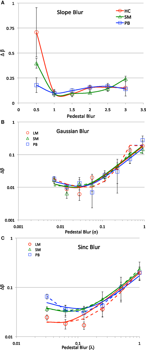
Figure 2. Blur discrimination thresholds for three observers, indicated in the legend and for three classes of blur (A) Amplitude Spectral Slope; (B) Gaussian, and (C) Sinc. The abscissa shows the level of blur present in the standard image, the ordinate show the change in blur required for detection of the more blurred image on 75% trials. Error bars show ±95% confidence intervals.
Dipper functions have frequently been reported for contrast discrimination as a function of pedestal contrast (Legge, 1981). For contrast discrimination, dipper functions are usually fit with first derivative of a sigmoidal contrast response function (e.g., Wilson, 1980 for review see Solomon, 2009). We could have fit the present data with a similar approach, but this would require the assumption that blur is represented in the human visual system by an analogous transducer function for image blur. We felt that it is unlikely that the visual system has any mechanisms that represent blur in this manner and we are not aware of any electrophysiological evidence for such neural populations.
Instead, we adapt a variance discrimination model, inspired by Morgan, Chubb and Solomon (Morgan et al., 2008) who used this approach to model mean orientation discrimination in images composed of oriented micro-patterns. The solid curves in Figures 2B,C show the fits of a variance discrimination model that is based on the additivity of variance:

where σe is the external blur (pedestal) applied to the stimulus, σi is the subject’s intrinsic blur and Ψ is the psychophysical threshold. Psychophysical threshold, Ψ, is defined as the proportional change in variance required for reliable discrimination of the standard and test images. The model assumes that there is a minimum level of intrinsic blur in the observer’s visual system, σi, arising from all optical and neurological sources. Thus, the representation of any edge, however sharp or blurred, is additionally subject to intrinsic blurring by the observer’s visual system. The variance of this noise ( ) sums with the variance of the blur applied to the standard (
 ) and test images (
 ), which can be discriminated when they differ by more than a fixed proportion (Ψ) that does not change with blur level. The fits in Figures 2B,C were obtained by maximum likelihood fit, weighted by the error bars on each data point, to estimate the values of σi and Ψ for each observer. The value of the threshold term, Ψ, and the internal blur parameter, σi, were the same for fits to both Gaussian and Sinc blur discrimination data. These parameters were fixed for each observer because they are inherent in the observer’s visual system and should not be expected to change with input. The external (pedestal) blur of the Gaussian-blurred edges (σe) is defined by the staircase program. There is no equivalent value for the standard deviation of the external blur for the Sinc filter. However, we can estimate this value by allowing the external noise parameter (σe) to vary and fixing the internal noise parameter (σi) for both Gaussian- and Sinc-blurred edges. This gives us a total of 1½ free parameters per fit for each observer. The estimate of equivalent external blur for Gaussian and Sinc filters provided an independent measure of the relative effective blur of these two blur methods. The data capture the main trends in the data with reasonable values of σi = 0.033° (0.02) and Ψ = 0.32 (0.15) mean (standard deviation) across all observers and conditions. The effective blur of the Gaussian and Sinc filters (λ/σ) was found to be 2.9 (0.81), in close agreement with the value identified in Experiment 2 in a matching task (see below).
The dashed curves in Figures 2B,C show the fits of a contrast discrimination model recently proposed by Watson and Ahumada (2010). The model is based on the assumption that a pair of blurred edges can be discriminated when the high spatial frequency components that differentiate them can be detected. A dipper function for blur discrimination emerges because following the contrast sensitivity function (Campbell and Robson, 1968), sensitivity is highest for intermediate blurred edge pairs whose spatial difference spectra peaks close to peak contrast sensitivity (typically close to 4 c/degree). The difference spectra for sharp or highly blurred edge pairs have spatial frequency peaks at higher and lower spatial frequencies respectively, where contrast sensitivity is reduced (Campbell and Robson, 1968). The dashed curves in Figures 2B,C were obtained by finding the peak spatial frequency of the difference between a standard Gaussian- or Sinc-blurred edge as in Experiment 1 and a test blurred edge that differed by a Weber fraction that was varied from 1/16 to ½ in log steps. Interestingly, the peak difference frequency was relatively invariant of the Weber fraction over this range, so we took the mean peak frequency of the estimates. A standard four parameter contrast sensitivity function (Watson, 2000) was used to estimate contrast detection thresholds for the peak spatial frequency for each pair of blurred edges. Superior fits were obtained when the same process was applied with a log double Gaussian contrast sensitivity function was employed:
where ω is spatial frequency, ωpeak is the spatial frequency with highest sensitivity, γ is maximum sensitivity and σh and σl, respectively determine the rate of sensitivity loss at high and low spatial frequencies. This function was better able to capture the rapid drop in contrast sensitivity at low spatial frequencies than the standard function that was required to fit the rising part of the dipper function. Such a rapid loss in contrast sensitivity to low spatial frequencies in images with natural amplitude spectra is consistent with our recent data in real images (Bex et al., 2009) and suggests that the presence of low spatial frequencies in blurred images may produce a similar loss in sensitivity to low spatial frequencies. The contrast detection model provided good fits to the blur discrimination data (dashed curves, Figures 2B,C), but required four free parameters per curve. We were unable to fit both the Gaussian and Sinc blur data with the same contrast sensitivity function for each observer.
In previous studies of slope discrimination, a similar minimum in discrimination threshold was observed at slopes around 1.2–1.4 (Hansen and Hess, 2006). The images employed in that study were of natural scenes, so it is difficult to relate blur to the slope of the amplitude spectrum, however, our data are in good general agreement with their observations of best sensitivity for slopes near those observed in images of natural scenes. For the slope-filtered images, unlike Gaussian or Sinc filtered images, we were able to examine blur discrimination thresholds for images that were over-sharpened, producing edges that are rarely, if ever, encountered under natural conditions. This allowed us to examine discrimination thresholds at positive and negative distances from a naturally sharp image. The slope blur discrimination data (Figure 2A) overwhelmingly show that thresholds for over sharp images, where the spectral slope has been manipulated to a degree beyond that occurring in the natural environment, are significantly raised. Under these conditions, naïve observers reported that the over sharp image appeared “out of focus” and therefore selected the (over sharp) standard image rather than the test image as the more blurred. This suggests that methods that manipulate the amplitude spectrum in either direction away from the original produce edges that are perceived as defocused or blurred, and not “over-sharp” as is often claimed. Lacking any theoretical basis for blur discrimination of slope manipulated images, we therefore did not attempt to fit the data with any variants of the variance or contrast discrimination models.
Experiment 2 Blur Matching
In Experiment 2, we attempt to obtain a qualitative match among the three classes of Slope, Gaussian and Sinc blurring methods. We attempted to generate matches between slope-filtered images and either of the other two methods. However, as can be seen in Figure 1A, slope filtering produces the qualitative appearance of a low contrast sharp edge that lies transparently over a low-pass filtered, hazy background. In pilot trials observers were unable to generate a satisfactory match between this class of image blur with either Gaussian or Sinc filtered images, so we did not pursue these matches and instead obtained matches between Gaussian and Sinc filtered edges.
The methods were similar to those used in Experiment 1. A new contoured source image was generated each trial from a binarized low-pass filtered noise image. The standard image was either Gaussian blurred with a standard deviation, σ, that was fixed at 1, 2, or 4 c/degree (8, 16, or 32 cycles per image) or Sinc-blurred with a reversal frequency, λ, that was fixed at 2, 4, or 8 c/degree (16, 32, or 64 cycles per image). When the standard was Gaussian blurred, the match was Sinc blurred and when the standard was Sinc blurred, the match was Gaussian blurred. The blur parameter of the match image (σ or λ) was under the control of a two-down-two-up staircase (Wetherill and Levitt, 1965) designed to converge at a blur level producing 50% “standard more blurred” responses. Both match types were interleaved in a single run, so that the observer was unaware which was the standard and which the match on any trial, even if they had been able to discriminate edges that were Gaussian or Sinc filtered. The staircases were initialized with random start values within ±4 dB of a value that minimized the difference between the amplitude spectra of the filters (see Figure 4); the step size was initially 2 dB and was reduced to 1 dB after two reversals. The standard and match images were independently assigned a RMS contrast randomly drawn from a normal distribution with a mean of 0.3 and a standard deviation of 0.1. This randomization of contrast ensured that observers could not reliably base their blur estimates on image contrast. The observer’s task was to indicate whether the more blurred image was on the left or right of fixation, there was no feedback. The raw data from a minimum of four runs for each condition (at least 160 trials per psychometric function) were combined and fit with a cumulative normal function by minimization of chi-square. Blur match thresholds were estimated from the 50% point of the best-fitting psychometric function and 95% confidence intervals on this point were calculated with a bootstrap procedure (Foster and Bischof, 1991).
Results and Discussion
Figure 3 shows blur matches between Gaussian- and Sinc-blurred edges for five observers, the authors and three observers who were naïve to the hypotheses of the experiment. Figure 3A shows data in which the standard image was Gaussian blurred with standard deviation fixed at 1, 2, or 4 c/degree and the match image was Sinc blurred whose blur parameter (λ) was adjusted according to the subject’s responses. Figure 3B shows data for the complimentary case in which the blur of the Sinc filtered image was fixed and the blur of Gaussian-blurred image was adjusted. The match values in both cases are expressed as the ratio of λ/σ that produced an edge of apparently equal blur, i.e., the standard image was perceived as more blurred than the match on 50% trials. Error bars show 95% confidence intervals. The horizontal lines in Figure 3 illustrate the expected blur matches based on four possible methods of blur estimation, illustrated in Figure 4.
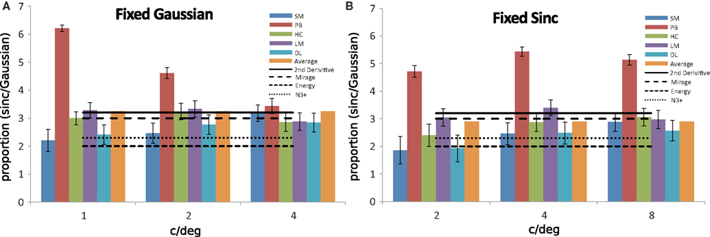
Figure 3. Blur matches between Gaussian- and Sinc-blurred edges for five observers, indicated by the caption. The y axis shows the ratio of λ/σ that produced an edge of matching blur when (A) the standard edge was Gaussian blurred with a fixed standard deviation of 1, 2, or 4 c/degree or (B) the standard edge was Sinc blurred with a standard deviation of 2, 4, or 8 c/degree. Error bars show ±95% confidence intervals.
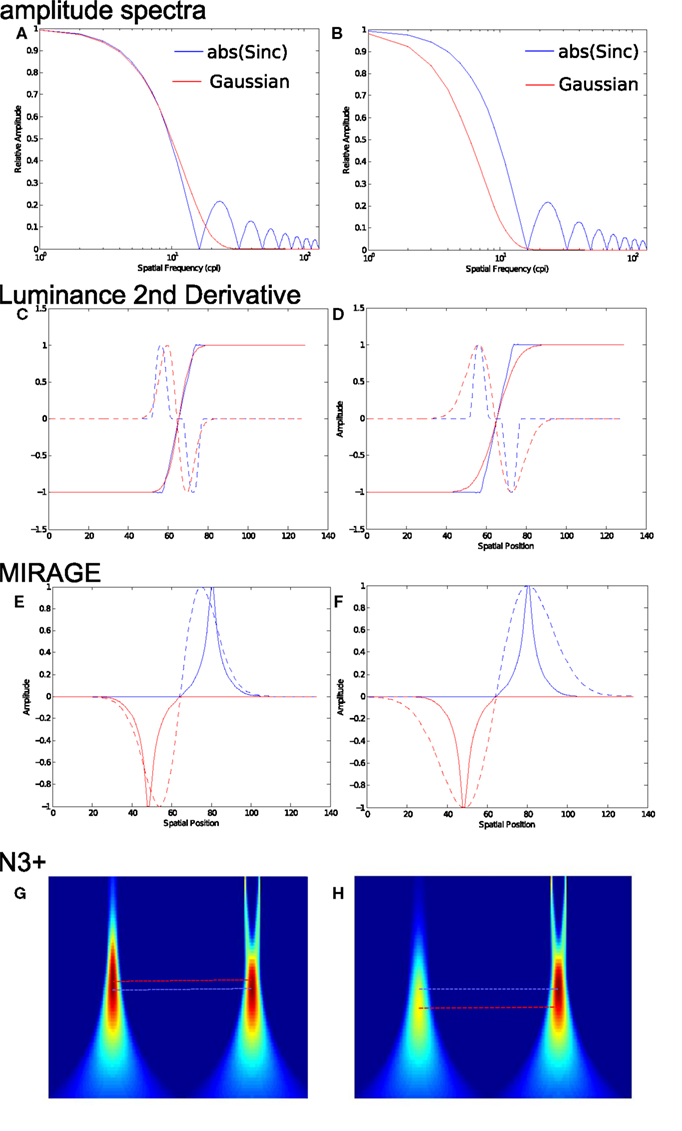
Figure 4. Illustration of four methods for the calculation of apparent blur: Amplitude spectrum, second derivative of luminance, MIRAGE and N3+. (A) The amplitude spectrum of a Sinc filter (blue curve, absolute valued with λ = 16 cpi) and the best-fitting Gaussian (red curve, σ = 8.1 cpi). (B) The same Sinc filter (blue curve, real valued λ = 16 cpi) and a more blurring Gaussian (red curve, σ = 5 cpi). (C) Convolution of a step edge with the filters in (A) produces blurred edges (C, solid curves) with similar peak slopes, but with second spatial derivatives (C, dashed curves) and zero bounded regions (ZBRs E, dashed curves) in MIRAGE whose peaks are closer together for the Gaussian- than the Sinc-blurred edge. (G) The peak responses of the N3+ model differs for the Gaussian (left fpeak = 7.2 pixels) and Sinc (right fpeak = 8.3 pixels) blurred edges. All three image-based models therefore correctly predict that the Sinc-blurred edge would appear more blurred than the Gaussian-blurred edge. (D) Convolution of a step edge with the mismatched filters in (B) produces blurred edges (D, solid curves) with similar peak slopes, but with different second spatial derivatives (D, dashed curves) and ZBRs (F) whose peaks are in the same locations for the Gaussian- and the Sinc-blurred edges. Dashed lines represent Gaussian and solid lines represent Sinc-blurred edges. (H) The peak responses of the N3+ model for the Gaussian (left fpeak = 11.5 pixels) and Sinc (right fpeak = 8.3 pixels) incorrectly predict that the Gaussian edge should now appear more blurred.
1. The first blur matching estimate assumes that perceived blur depends on the relative energy at high spatial frequencies. This method is illustrated in Figure 4A, which shows best least-squares fitting Gaussian (red curve, σ = 8.1 cpi) to the absolute valued Sinc function (λ = 16 cpi). The absolute value of the amplitude spectrum has been used because this model is not affected by phase or the spatial structure of the image formed, only the energy at different spatial frequencies. The solid lines in Figure 4C show the 1D profile of a step edge that has been blurred with the filters shown in Figure 4A – the red edge has been filtered by the red Gaussian in Figure 4A, the blue edge by the blue Sinc function in Figure 4A. The profiles of the edges are quite similar, as are their slopes. Any model based on the relative amplitude of structure across spatial scales predicts that these two edges should appear similarly blurred. This matching point for this method is indicated by the horizontal short dashed line in Figures 3A,B (see caption). Our results show that the apparent blur of these edges does not match. Figure 4B shows the same Sinc function (λ = 16 cpi, blue curve) together with a Gaussian (red curve, σ = 5 cpi). The solid lines in Figure 4D show the 1D profile of a step edge that has been blurred with the filters shown in Figure 4B – the red edge has been filtered by the red Gaussian in Figure 4B, the blue edge by the blue Sinc function in Figure 4B. Any model based on the relative amplitude of structure across spatial scales predicts that these two edges should not appear equally blurred. Our results, however, show that they do.
Note that the Gaussian fit to the Sinc profile tends to underestimate the presence of oscillating high spatial frequency structure in Sinc-blurred edges. If anything, these high spatial frequency components should tend to make Sinc edges appear slightly sharper, the opposite to the effects we observe and making our matching estimate conservative.
2. The second blur matching estimate assumes that perceived blur depends on the separation between peaks in the second spatial derivative (Marr and Hildreth, 1980). The dashed lines in Figures 4C,D show the second derivatives of the correspondingly colored edges (solid lines) in those figures. For esthetic purposes, the plots have been smoothed with Matlab’s Lowess linear local regression method, which does not affect the location of the largest peaks. The zero crossing of the second derivative is routinely used to indicate the location of an edge of arbitrary blur (Marr and Hildreth, 1980) and in both cases the zero crossing falls in the perceived and physical location of the edge. The peaks of the second derivative define a distribution that can be used to estimate image blur (Watt and Morgan, 1985). The peaks in Figure 4C are closer together for the Gaussian-blurred than the Sinc-blurred edges. Thus the second derivative model predicts that the Sinc-blurred edge should appear more blurred than the Gaussian-blurred edge, consistent with our data. Figure 4D shows the second spatial derivative of the edges produced by the filters shown in Figure 4B, with correspondingly colored dashed curves. The peaks in the second derivative now occur in the same location, so this model predicts that these two edges should appear equally blurred. This matching point is indicated by the horizontal solid lines in Figures 3A,B and this is in good agreement with the matches obtained in the experiment.
3. The third blur matching estimate implements the MIRAGE model and assumes that perceived blur depends on the separation between peaks in the summed outputs of a bank of narrow-band filters (Watt and Morgan, 1985). We implemented the model with a bank of four narrow band filters, each was the second derivative of a Gaussian with a standard deviation from 1.875 to 15 arcmin (1–8 pixels) in four log steps. The output of each filter was normalized between −1 and +1 and the positive values were summed separately from negative values across spatial scales. The separation between peaks in the summed outputs was taken as the extent of blur. Figures 4E,F illustrate the output for the Gaussian- and Sinc-blurred edges shown in Figures 4C,D using the filters shown in Figures 4A,B respectively. The matching point of the MIRAGE model is indicated by the horizontal long dashed lines in Figures 3A,B. The predictions are close to the second derivative of luminance and are thus in good agreement with the data.
4. The fourth estimate of blur implements the  model (Georgeson et al., 2007). This model involves the analysis of cascaded rectified Gaussian derivative filter pairs and identifies the location and blur of an edge from the location of the peak in the response distribution to a given image. The model was implemented with the parameters from the original paper (Georgeson et al., 2007). The image was processed in a series of channels with Gaussian standard deviation (σ) from 1 to 64 pixels in 64 log spaced steps. The image was first convolved with a family of scale-normalized first derivative Gaussian filters with a standard deviation, σ1, fixed at σ/4. The rectified output of each filter was scaled by
  and convolved with paired third derivative Gaussian filters whose standard deviation,
  , before scaling by
  . The peak response across the image and across the bank of filters was used to read off the location of edge and its blur extent. Figures 4G,H illustrate the output for the 1D edges shown in Figures 4C,D. The left distributions in G and H show the response to the Gaussian edge, the right distributions show the response to the Sinc edge. The model correctly identifies the location of the edge and predicts that the Sinc edge in Figure 4A (σ fpeak = 8.3 pixels) is more blurred than the Gaussian edge (σ fpeak = 7.2 pixels). However, for the subjectively matched edge in Figure 4B, the model predicts a difference in apparent blur: σ fpeak = 11.3 pixels for the Gaussian and σ fpeak = 8.3 pixels for the Sinc-blurred edge. The matching point of the
  model is indicated by the horizontal dotted lines in Figures 3A,B.
General Discussion
This paper examined the blur of edges manipulated by common empirical and computational methods. The most common methods of manipulating blur in digital image processing involve progressively attenuating the amplitude of high spatial frequency components by changing the slope of the amplitude spectrum or the use of Gaussian operators. Neither of these methods changes the phase spectrum of the blurred image. The most common sources of image blur in the natural environment, however, arise from changes in pupil diameter or accommodation. These sources of natural image blur change not only the amplitude spectrum of the image, but also introduce systematic changes in the phase spectrum. Optical and aperture blur cause non-monotonic attenuation of amplitude at higher spatial frequencies and periodic 180° reversals in phase. In Experiments 1 and 2, we examine how these differences affect perceived blur.
Experiment 1 measured blur discrimination thresholds for three methods of manipulating image blur. For Gaussian- and Sinc-blurred images, discrimination thresholds were dipper shaped, in line with several previous studies (Hamerly and Dvorak, 1981; Watt and Morgan, 1983; Paakkonen and Morgan, 1994; Wuerger et al., 2001; Mather and Smith, 2002). The results were well characterized by a contrast discrimination model (Watson and Ahumada, 2010) and by a variance discrimination model, adapted from a similar model developed for orientation discrimination (Morgan et al., 2008; Solomon, 2009). The contrast discrimination model assumes that blurred edges can be discriminated when the differences in their amplitude spectra can be detected. This model was able to capture the main trends in the data, but required different four-parameter contrast sensitivity functions in the same observer to fit the data for Gaussian- and Sinc-blurred edges. In the variance discrimination model, the overall level of blur represented by the visual system is the result of the combination of extrinsic blur in the image and intrinsic blur by the anterior stages of visual processing, including all optical and neural sources. The variances from these noise sources sum linearly and blur can be discriminated when the total variance of the standard and test intervals exceeds a threshold proportion. This simple model produced dipper functions for blur discrimination and provides a good fit to the data with only two shared parameters for each observer, both of which have biologically plausible values and importantly were the same for Gaussian and Sinc blur. Note that this model does not depend on non-linear transducer functions (Wilson, 1980) which, while reasonable for representing image contrast, are implausible for the representation of image blur. We speculate that this class of variance discrimination model may offer a general alternative to current approaches to fit dipper-shaped pedestal discrimination functions (Solomon, 2009).
For slope-filtered images, blur discrimination thresholds were highly non-linear. For slopes that were steeper (i.e., more blurred) than the original image, blur (slope) discrimination thresholds were relatively stable, with a small increase in thresholds with pedestal blur, in line with previous studies (Hansen and Hess, 2006). For slopes that were shallower (i.e., over-sharp) than the original, blur discrimination thresholds rose abruptly, indicating that observers may not perceive over-sharpened images on the same continuum as blurred images. Instead, we speculate that observers perceive any deviation away from the original sharp slope as “out of focus”, regardless of the direction of the change in slope. The absence of “over-sharp” stimuli in the natural environment makes digitally sharpened images highly atypical, so that any stimuli beyond the slope of “in focus” based on naturally occurring conditions appear alien and blurred. This observation has implications for efforts to determine satisfactory levels of image blur (Ciuffreda et al., 2006). Therefore, although the slope of the amplitude spectrum for images of natural scenes is a useful descriptor of their statistical properties, it may not be an ideal way of manipulating or quantifying the level of blur in the image. This conclusion is supported by Experiment 2, in which we attempted to match the apparent blur across the three classes of blur. We found that in comparing types of blur, Slope-blurred or sharpened images could not be matched with either Sinc or Gaussian-blurred images as its edges were not perceived as blurred but only as hazy and transparent.
Observers were, however, able to make satisfactory matches between Gaussian- and Sinc-blurred images. The blur matching results were not consistent with the estimate of blur obtained from the relative amplitude across spatial frequencies, suggesting that perceived blur is not simply dependent on the relative amplitude of spatial structure at high and low spatial scales. This observation is also consistent with the failure of the contrast detection model to predict blur discrimination thresholds with the same contrast sensitivity function for both Sinc- and Gaussian-blurred edges. Alternatively, the blur matching results were in good agreement with the match points predicted by the locations of peaks in the second spatial derivative of luminance and with the locations of zero bounded regions (ZBRs) in a MIRAGE model (Watt and Morgan, 1985), but not with the parameters of the  model, which is a similar filter channel. This result provides general support for some of the fundamental principles of the MIRAGE model (Watt and Morgan, 1985). A key assumption of MIRAGE is that spatial frequency filter responses cannot be separately accessed within the visual system but their outputs are combined before feature analysis. This assumes that analyses at separate spatial scales of the visual system sum before analysis can occur. To model this process, MIRAGE first separates the positive and negative responses and half wave rectifies to preserve each frequency filter’s input. This results in the smallest filter output surviving the influence of larger filters. The model gives each filter equal weight regardless of size and as a result the model is more sensitive to high SF channels.
The ratio of the terms that control the level of blur in Gaussian and Sin blurred images is expressed in this study as λ/σ. The precise value of this ratio is not important, but it is significant that the ratio that fit the blur discrimination data in the variance discrimination fits of Experiment 1 and the blur matching data in Experiment 2 is approximately the same.
Owing to the difficulties of quantifying blur in images of natural scenes, we employed synthetic images that shared some of the spatial properties of natural images, including the amplitude spectrum as well as two-dimensional orientation and curvature properties examined in the Appendix. While the use of these images allowed us to control blur directly, there remain significant differences between the noise images employed in the present study and images of real scenes. Firstly, the distribution of luminance and contrast in the present images was uniform, whereas in natural images, luminance and contrast are highly non-uniform (Ruderman and Bialek, 1994; Balboa and Grzywacz, 2000, 2003; Mante et al., 2005; Frazor and Geisler, 2006) and these parameters are known to affect perceived blur (May and Georgeson, 2007a,b). Secondly, the contours in the present stimuli were shorter and less numerous than those in natural images and we do not know how these properties affect perceived blur. We are therefore currently studying perceived blur in more complex synthetic images in which we can also control these parameters as well as local blur. This will allow us to examine how these differences affect apparent blur in images that more closely resemble natural images.
Conclusions
Collectively, our results show that the simple presence of high spatial frequencies in an image does not guarantee that the image will appear more sharp or less blurred. Indeed, in cases in which the slope of the amplitude spectrum is made shallower, the image may actually appear qualitatively more out of focus. Furthermore, we have shown that the presence of phase reversed high spatial frequencies in Sinc-blurred edges can result in an image that appears more blurred than a Gaussian-blurred image with a similar amplitude spectrum. This is contrary to the common assumption that blurring of images is caused by an overall reduction of the total energy at high spatial frequencies and that sharpening an image requires an overall increase in the relative amplitude of high spatial frequencies.
This has implications for the future study of perceived blur in natural images. While the slope of the amplitude spectrum is commonly used to manipulate image blur in natural scenes, our results suggest that this method does not necessarily modify perceived blur in the manner that is assumed by this approach. Digital image blurring with Gaussian and Sinc profile filters can generate blurred images with broadly similar amplitude spectra, however these images may appear to have dissimilar levels of perceived blur. These observations emphasize the importance of the phase of high spatial frequencies that may have been underestimated previously.
Conflict of Interest Statement
The authors declare that the research was conducted in the absence of any commercial or financial relationships that could be construed as a potential conflict of interest.
Acknowledgment
Supported by NEI R01 EY019281.
References
Balboa, R. M., and Grzywacz, N. M. (2000). Occlusions and their relationship with the distribution of contrasts in natural images. Vision Res. 40, 2661–2669.
Balboa, R. M., and Grzywacz, N. M. (2003). Power spectra and distribution of contrasts of natural images from different habitats. Vision Res. 43, 2527–2537.
Bex, P. J., and Makous, W. (2002). Spatial frequency, phase, and the contrast of natural images. J. Opt. Soc. Am. A 19, 1096–1106.
Bex, P. J., Solomon, S. G., and Dakin, S. C. (2009). Contrast sensitivity in natural scenes depends on edge as well as spatial frequency structure. J. Vis. 9, 1–19.
Billock, V. A., de Guzman, G. C., and Kelso, J. A. S. (2001). Fractal time and 1/f spectra in dynamic images and human vision. Phys. D 148, 136–146.
Brady, N., Bex, P. J., and Fredericksen, R. E. (1997). Independent coding across spatial scales in moving fractal images. Vision Res. 37, 1873–1883.
Burton, G. J., and Moorhead, I. R. (1987). Color and spatial structure in natural scenes. Appl. Opt. 26, 157–170.
Campbell, F. W., and Robson, J. G. (1968). Application of Fourier analysis to the visibility of gratings. J. Physiol. Lond. 197, 551–566.
Canny, J. A. (1986). Computational approach to edge detection. IEEE Trans. Pattern Anal. Mach. Intell. 8, 679–714.
Ciuffreda, K. J., Selenow, A., Wang, B., Vasudevan, B., Zikos, G., and Ali, S. R. (2006). “Bothersome blur”: a functional unit of blur perception. Vision Res. 46, 895–901.
Field, D. J. (1987). Relations between the statistics of natural images and the response properties of cortical cells. J. Opt. Soc. Am. A 4, 2379–2394.
Foster, D. H., and Bischof, W. F. (1991). Thresholds from psychometric functions: superiority of bootstrap to incremental and probit variance estimators. Psychol. Bull. 109, 152–159.
Frazor, R. A., and Geisler, W. S. (2006). Local luminance and contrast in natural images. Vision Res. 46, 1585–1598.
Freeman, W. T., and Adelson, E. H. (1991). The design and use of steerable filters. IEEE Trans. Pattern Anal. Mach. Intell. 13, 891–906.
Geisler, W. S., Perry, J. S., Super, B. J., and Gallogly, D. P. (2001). Edge co-occurrence in natural images predicts contour grouping performance. Vision Res. 41, 711–724.
Georgeson, M. A., May, K. A., Freeman, T. C., and Hesse, G. S. (2007). From filters to features: scale-space analysis of edge and blur coding in humanvision. J. Vis. 7, 1–21.
Gonzalez, R. C., Woods, R. E., and Eddins, S. L. (2004). Digital Image Processing Using MatLab. Upper Saddle River, NJ: Pearson Prentice Hall.
Hamerly, J. R., and Dvorak, C. A. (1981). Detection and discrimination of blur in edges and lines. J. Opt. Soc. Am. 71, 448–452.
Hansen, B. C., and Hess, R. F. (2006). Discrimination of amplitude spectrum slope in the fovea and parafovea and the local amplitude distributions of natural scene imagery. J. Vis. 6, 696–711.
Hodos, W., and Kuenzel, W. J. (1984). Retinal-image degradation produces ocular enlargement in chicks. Invest. Ophthalmol. Vis. Sci. 25, 652–659.
Hubel, D. H., and Wiesel, T. N. (1968). Receptive fields and functional architecture of monkey striate cortex. J. Physiol. 195, 215–243.
Mante, V., Frazor, R. A., Bonin, V., Geisler, W. S., and Carandini, M. (2005). Independence of luminance and contrast in natural scenes and in the early visual system. Nat. Neurosci. 8, 1690–1697.
Marr, D., and Hildreth, E. (1980). Theory of edge detection. Proc. R. Soc. Lond., B, Biol. Sci. 207, 187–217.
Mather, G., and Smith, D. R. (2002). Blur discrimination and its relation to blur-mediated depth perception. Perception 31, 1211–1219.
May, K. A., and Georgeson, M. A. (2007a). Added luminance ramp alters perceived edge blur and contrast: a critical test for derivative-based models of edge coding. Vision Res. 47, 1721–1731.
May, K. A., and Georgeson, M. A. (2007b). Blurred edges look faint, and faint edges look sharp: the effect of a gradient threshold in a multi-scale edge coding model. Vision Res. 47, 1705–1720.
Morgan, M., Chubb, C., and Solomon, J. A. (2008). A “dipper” function for texture discrimination based on orientation variance. J. Vis. 8, 1–8.
Morgan, M. J., Ross, J., and Hayes, A. (1991). The relative importance of local phase and local amplitude in patchwise image-reconstruction. Biol. Cybern. 65, 113–119.
Morgan, M. J., and Watt, R. J. (1997). The combination of filters in early spatial vision: a retrospective analysis of the MIRAGE model. Perception 26, 1073–1088.
Oppenheim, A. V., and Lim, J. S. (1981). The importance of phase in signals. Proc. IEEE 69, 529–541.
Paakkonen, A. K., and Morgan, M. J. (1994). Effects of motion on blur discrimination. J. Opt Soc. Am. 11, 992–1002.
Pelli, D. G. (1997). The VideoToolbox software for visual psychophysics: transforming numbers into movies. Spat. Vis. 10, 437–442.
Piotrowski, L. N., and Campbell, F. W. (1982). A demonstration of the visual importance and flexibility of spatial-frequency amplitude and phase. Perception 11, 337–346.
Ruderman, D. L., and Bialek, W. (1994). Statistics of natural images: scaling in the woods. Phys. Rev. Lett. 73, 814–817.
Tadmor, Y., and Tolhurst, D. J. (1993). Both the phase and the amplitude spectrum may determine the appearance of natural images. Vision Res. 33, 141–145.
Thomson, M. G. A., Foster, D. H., and Summers, R. J. (2000). Human sensitivity to phase perturbations in natural images: a statistical framework. Perception 29, 1057–1069.
Tolhurst, D. J., and Tadmor, Y. (1997). Discrimination of changes in the slopes of the amplitude spectra of natural images: band-limited contrast and psychometric functions. Perception 26, 1011–1025.
Tyler, C. W. (1997). Colour bit-stealing to enhance the luminance resolution of digital displays on a single pixel basis. Spat. Vis. 10, 369–377.
van Hateren, J. H., and van der Schaaf, A. (1998). Independent component filters of natural images compared with simple cells in primary visual cortex. Proc. R. Soc. Lond., B, Biol. Sci. 265, 359–366.
Vera-Diaz, F. A., Woods, R. L., and Peli, E. (2010). Shape and individual variability of the blur adaptation curve. Vision Res. 50, 1452–1461.
Wallman, J., Turkel, J., and Trachtman, J. (1978). Extreme myopia produced by modest change in early visual experience. Science 201, 1249–1251.
Watson, A. B. (2000). Visual detection of spatial contrast patterns: evaluation of five simple models. Opt. Express 6, 12–33.
Watt, R. J., and Morgan, M. J. (1983). The recognition and representation of edge blur: evidence for spatial primitives in human vision. Vision Res. 23, 1465–1477.
Watt, R. J., and Morgan, M. J. (1985). A theory of the primitive spatial code in human vision. Vision Res. 25, 1661–1674.
Webster, M. A., Georgeson, M. A., and Webster, S. M. (2002). Neural adjustments to image blur. Nat. Neurosci. 5, 839–840.
Wetherill, G. B., and Levitt, H. (1965). Sequential estimation of points on a psychometric function. Br. J. Math Stat. Psychol. 18, 1–10.
Wilson, H. R. (1980). A transducer function for threshold and suprathreshold human vision. Biol. Cybern. 38, 171–178.
Woods, R. L., Colvin, C. R., Vera-Diaz, F. A., and Peli, E. (2010). A relationship between tolerance of blur and personality. Invest. Ophthalmol. Vis. Sci.
Keywords: blur, phase, contours, variance, contrast, amplitude spectrum, orientation
Citation: Murray S and Bex PJ (2010) Perceived blur in naturally contoured images depends on phase. Front. Psychology 1:185. doi: 10.3389/fpsyg.2010.00185
Received: 14 June 2010;
Paper pending published: 14 September 2010;
Accepted: 11 October 2010;
Published online: 02 December 2010.
Edited by:
Sheng He, University of Minnesota, USACopyright: © 2010 Murray and Bex. This is an open-access article subject to an exclusive license agreement between the authors and the Frontiers Research Foundation, which permits unrestricted use, distribution, and reproduction in any medium, provided the original authors and source are credited.
*Correspondence: Peter J. Bex, Department of Ophthalmology, Schepens Eye Research Institute, Harvard Medical School, 20 Staniford Street, Boston, MA, USA. e-mail: peter.bex@schepens.harvard.edu