Non-Stationarity in Multisensory Neurons in the Superior Colliculus

The superior colliculus (SC) integrates information from multiple sensory modalities to facilitate the detection and localization of salient events. The efficacy of “multisensory integration” is traditionally measured by comparing the magnitude of the response elicited by a cross-modal stimulus to the responses elicited by its modality-specific component stimuli, and because there is an element of randomness in the system, these calculations are made using response values averaged over multiple stimulus presentations in an experiment. Recent evidence suggests that multisensory integration in the SC is highly plastic and these neurons adapt to specific anomalous stimulus configurations. This raises the question whether such adaptation occurs during an experiment with traditional stimulus configurations; that is, whether the state of the neuron and its integrative principles are the same at the beginning and end of the experiment, or whether they are altered as a consequence of exposure to the testing stimuli even when they are pseudo-randomly interleaved. We find that unisensory and multisensory responses do change during an experiment, and that these changes are predictable. Responses that are initially weak tend to potentiate, responses that are initially strong tend to habituate, and the efficacy of multisensory integration waxes or wanes accordingly during the experiment as predicted by the “principle of inverse effectiveness.” These changes are presumed to reflect two competing mechanisms in the SC: potentiation reflects increases in the expectation that a stimulus will occur at a given location relative to others, and habituation reflects decreases in stimulus novelty. These findings indicate plasticity in multisensory integration that allows animals to adapt to rapidly changing environmental events while suggesting important caveats in the interpretation of experimental data: the neuron studied at the beginning of an experiment is not the same at the end of it.

Introduction

There is a significant difference in the way that we think about the brain and the way in which we conduct experiments and analyze data. While we appreciate that the brain is malleable and adapts to experience, we know that neural activity can be random, and we draw our conclusions from analyses that require data to be averaged over multiple trials. In the study of sensory neurophysiology, we commonly attempt to attenuate adaptation to different stimuli by randomly interleaving their presentation. But is the neuron at the beginning of the experiment in the same state at the end given these efforts?

We found that, in the case of superior colliculus (SC) neurons, it is not. The SC is unique in that it is capable of integrating information from multiple sensory modalities (Stein and Arigbede, 1972; Stein and Dixon, 1979; Meredith and Stein, 1983, 1986; King and Palmer, 1985; Meredith et al., 1992; Peck et al., 1993; Stein and Meredith, 1993; Wallace et al., 1993, 1996; Wallace and Stein, 2001; Populin and Yin, 2002; Perrault et al., 2003; Alvarado et al., 2008, 2009; Zahar et al., 2009). The SC contains multisensory neurons that receive unisensory signals from independent channels and integrate that information in the form of response enhancements and depressions. This integrative capacity makes them well suited for stimulus detection and localization (Jay and Sparks, 1987; Lee et al., 1988; Frens and Van Opstal, 1998; Jiang et al., 2002; Burnett et al., 2004; Bell et al., 2005). The most common method to assess these enhancements and depressions employ techniques that evaluate the averaged activity of these neurons to both modality-specific and cross-modal stimuli over many trials. While integrative responses are clearly demonstrated throughout the literature, it is also apparent that neurons within the SC exhibit substantial variation in activity levels across the population as well as within the responsivity of a single neuron. We sought to explore how the changes in an individual neuron’s responsivity might be explained. Our fundamental hypothesis is that it reflects two opposing forces, one that promotes the detection of weakly effective stimuli, and another that demotes responses to strongly effective stimuli. We predicted that there would be fluctuations in the responses of SC neurons during an experiment, with the specific prediction that strong responses would decrease in magnitude (“habituate”), while weak responses would increase (“potentiate”).

In an analysis of an extensive dataset (n = 110) in which multisensory neurons in the SC were presented with visual, auditory, and visual–auditory combinations of stimuli, we found significant changes in their response magnitudes that were consistent with our principal hypothesis (i.e., strong responses habituated, weak responses potentiated). These trends were not due to random fluctuations. As a consequence, the “benefit” provided by integrating signals across sensory channels (“multisensory integration”) changed during the course of the experiment in a manner consistent with the “principle of inverse effectiveness” (Meredith et al., 1987; Stein and Stanford, 2008). The potency of multisensory integration is therefore not constant in time either during a response (Rowland et al., 2007), or over the course of an experiment.

Instead, unisensory and multisensory responses are not stationary, an observation that is consistent with recent findings (see Yu et al., 2009). However, unlike that study, the dataset analyzed here was recorded under experimental conditions designed to attenuate such changes. Predictable changes occurred despite these efforts, thereby revealing another aspect by which inherent neural plasticity can have a substantial impact on the way in which we interpret data.

Materials and Methods

All procedures were carried out in accordance with the National Institutes of Health guidelines for animal research and were in compliance with an approved protocol at the Wake Forest University School of Medicine, which is accredited by the American Association for the Accreditation of Laboratory Animal Care. Experiments were performed in three adult cats weighing 2.5–5.0 kg. Animals were prescreened for normal vision and hearing prior to inclusion in the study.

Implantation Procedure

An initial surgical procedure was performed placing a recording well/head-holding device on the skull prior to any electrophysiology recordings (McHaffie and Stein, 1983). Animals were initially rendered tractable with an intramuscular injection of ketamine HCl (20 mg/kg) and acepromazine maleate (0.2–0.4 mg/kg). A steady plane of anesthesia maintained using isoflurane (1–4%) following endotracheal intubation. Throughout the surgery, hydration was maintained with intravenous infusion of lactated Ringer solution (4–8 ml/h) via the saphenous vein. This was followed by postsurgical subcutaneous administration of lactated Ringer (30 ml/kg). Expiratory CO₂ and temperature were monitored to remain within normal limits. Eyes were protected with constant application of sterile artificial tears to prevent corneal drying during the duration of the procedure. Once anesthetized, the animal was placed in a stereotaxic frame, and a craniotomy exposed the cortex overlying the SC. A stainless steel chamber that provides access to the SC as well as holds the head was affixed to the skull using stainless steel bone screws and orthopedic bone cement. Analgesics (butorphanol 0.1–0.4 mg/kg or ketoprofen 1–2 mg/kg) were given as needed during recovery.

General Recording Procedure

During electrophysiological recordings the animal was rendered tractable with an intramuscular injection of ketamine (20 mg/kg) and acepromazine (0.4 mg/kg). Animals were intubated and stabilized in a head holder without wounds or pressure points. A cannula was placed in the saphenous vein for the continuous delivery of anesthetic (ketamine: 4–8 mg/kg/h), paralytic (pancuronium bromide: 0.2 mg/kg/h), and fluids (lactated Ringer: 4–8 ml/h). Paralysis and artificial respiration are necessary because eye movements can produce significant displacement of visual receptive fields. Maintenance of adequate levels of anesthesia was done by monitoring multiple vital signs, including expiratory CO₂, heart rate, and blood pressure. For purposes of receptive field mapping, the pupils were dilated with 1% atropine sulfate and corrective contact lenses were placed on the anesthetized (0.5% proparacaine hydrochloride ophthalmic solution) corneas to adjust for retinoscopically determined refractive errors. The optic disks were rear-projected and focused onto a 91-cm-diameter translucent hemisphere placed 45 cm from the eyes. Receptive field maps acquired from multiple sessions in the same and different animals could then be registered by aligning the position of the optic disk. Individual animals underwent recording sessions 1–3 times per week. Anesthesia and paralytic was reversed and on return of normal respiration and locomotion, the animal was returned to its home cage. Experiments generally lasted between 8 and 12 h.

Neuronal Isolation and Recording

Tungsten microelectrodes (tip diameter: 1–3 μm, impedance: 1–3 MΩ at 1 kHz) were positioned with a Kopf micromanipulator and lowered into the intermediate layers of the SC. Position was confirmed by the characteristic visual activity elicited by the superficial layers. The electrode was advanced into stratum opticum (the transitional layer between the superficial and deep SC) by means of a hydraulic microdrive. From here, the electrode was advanced in 10-μm steps while presenting visual and auditory search stimuli as in previous studies (Meredith and Stein, 1986; Wallace et al., 1993). Single units were isolated (criterion signal: noise = 3:1) and digitized by means of a window discriminator (FHC). Neural activity was amplified and monitored, and data were collected using a customized suite of software that employs the 1401 Plus data acquisition system (Cambridge Electronic Design). In the current study, only visual–auditory multisensory neurons were examined.

Sensory Stimuli

Stationary visual stimuli consisted of the 50- to 100-ms illumination of a light-emitting diode (LED; 660 nm λ) placed within the receptive field (see Receptive Field Mapping). Moving visual stimuli consisted of slits, bars, or spots of light projected onto the translucent hemisphere, the movement speed, amplitude, and direction of which could be independently controlled. Whereas the intensity of stationary stimuli was computer controlled, the intensity of moving stimuli was controlled using neutral density filters. In both circumstances stimulus intensity ranged from 0.11 to 13.0 cd/m² with a background luminance of 0.10 cd/m². Auditory stimuli were delivered in a free-field setting and consisted of 50- to 100-ms duration broadband noise bursts (20 Hz–10 kHz). These stimuli were digitally synthesized and delivered through speakers that could be positioned at any location in auditory space. Auditory stimulus intensities ranged from 50.6 to 70.0 dB sound pressure level (SPL) against a background SPL of 50.0 dB. Visual and auditory intensities used for testing were determined by presenting a range of intensities that elicited a threshold response as well as a saturated response. Once this was determined visual and auditory stimuli were matched to create the cross-modal pair based upon their relative position along their unisensory saturation curve. Modality-specific and cross-modal stimuli were then presented randomly for a minimum of 15 trials at the most sensitive location within their respective excitatory receptive field. For all trials, neuronal activity was recorded for 2–3 s with a 500 ms interval prior to stimulus presentation. An interstimulus interval ranging from 5 to 10 s was used for each trial.

Receptive Field Mapping

The borders of each visual receptive field were mapped onto the translucent hemisphere by moving the optimum stimulus, projected from a handheld pantoscope, from the periphery inward from all directions until an enclosed responsive area was defined. Auditory receptive fields were mapped using brief (50 ms) broadband noise bursts delivered from a speaker that could be positioned at any location on a hoop that could be freely rotated about the animal’s interaural axis. The typical steps in speaker location represented ∼15° of auditory angle in both the azimuthal and elevation dimensions. The location of the stimulus was randomly varied, and a positive response (i.e., a location within the receptive field) was one in which the stimulus-evoked response was readily discernible above background activity. For purposes of receptive field mapping, auditory stimuli were 15 dB above the neuron’s previously determined threshold. Receptive fields were transposed from the hemisphere and plotted on standardized representations of visual and auditory space.

Data Analysis

Response magnitude was identified by first demarcating the onset and offset of the response using a three-step geometric method as in the past (Rowland et al., 2007). This “response window” was calculated using data from all trials from a particular stimulus presentation condition. The window of time 500 ms prior to stimulus onset was used to calculate the spontaneous rate. We then counted the number of impulses in the response window on each trial and subtracted the expected number given the size of the window and the spontaneous rate, producing a trial-by-trial estimate of response magnitude. A simple linear regression was used to determine the slope of the response magnitude vs. trial number trend.

Because it was possible, in principle, for any changes to be due to random fluctuations, the analysis had multiple levels. One would expect, based on random fluctuations, that responses that were randomly large on the first trial would be smaller on the last, and responses that were randomly small on the first trial would be larger on the last (“regression to the mean”). To compensate, in our analysis we examined how predictive the averages of the response magnitudes on the first few trials were of the overall trend. If averaging several initial trials still provided a better estimate relative to averaging all trials, then regression to the mean would be a less likely inference. This was tested with correlation values.

We then examined how predictive the response to a stimulus would be of the response when it was presented a second, third, or fourth time in the randomly interleaved series (i.e., with intervening stimuli). In a circumstance in which neural responses are random, the correlation coefficient should be randomly distributed in each of these comparisons. However, if the neural response is changing in a predictable way, then the first response should be a better predictor of the response to the second presentation than the third presentation. Again, correlation was used to quantify these relationships.

Finally, we compared the slopes of the changes in the multisensory responses to the best (i.e., largest) unisensory responses. If multisensory responses reflect fluctuations in the unisensory input magnitudes, there should be a correlation between these values according to the principle of inverse effectiveness. On the other hand, if the results were due to randomness, there would be no correlation: unisensory efficacy and multisensory efficacy would be unrelated in this comparison.

Results

The primary observation was that initially strong responses tended to get weaker, while weak responses got stronger, during the course of the experiment. This occurred for both unisensory and multisensory responses even when stimulus presentations were randomly interleaved in an attempt to suppress such changes. The results did not reflect random changes in the neuron’s responsiveness, because changes could be better predicted by averaging the responses on a few initial trials, response magnitudes on a given trial were better predicted by more proximate responses, and there was a good correlation between the changes observed in the multisensory and unisensory responses. As a consequence, the efficacy of multisensory integration during the course of an experiment changed in a predictable fashion (i.e., according to the principle of inverse effectiveness), because the neuron’s state at the beginning of the experiment was not the same at the end.

Neurons adapted rapidly in experiments where stimuli were randomly interleaved. Figure 1 gives examples of how responses in two neurons changed over the course of an experiment. As a neuron is given repeated exposure to a particular stimulus that initially elicits a weak response (Figures 1A,B), the response strengthens, even when these trials are interleaved with the presentation of other stimuli. On the other hand, when a neuron is given repeated exposure to a stimulus that initially elicits a strong response (Figures 1C,D), the response weakens. There is some random fluctuation in the actual response magnitude on a trial-by-trial basis, but the overall trend remains consistent and is exposed by the slope of the linear regression.

FIGURE 1

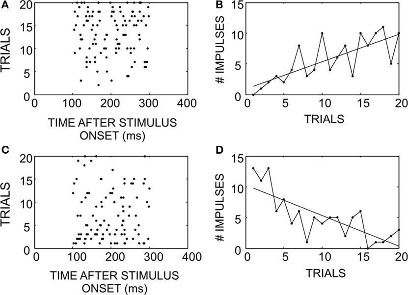
Figure 1. How SC neuronal responses change as a consequence of exposure to randomly interleaved stimuli. (A) An example of a response that begins weak, and potentiates over successive trials (ordered bottom-to-top). (B) Response magnitude changes on successive trials while there is some amount of noise, the overall trend increased the number of impulses elicited. (C) An example of a response that begins strong, but habituates over time. (D) Illustration of the response magnitude changes: negative, despite random trial-by-trial noise.

The population was examined to determine if these changes were consistent. Figure 2 shows the results of the primary analysis, in which the change (slope) of the response magnitude over trials is compared to the initial, averaged, and final response magnitudes. The first plot reveals the inverse correlation between the initial response magnitude and the slope of the response magnitude trend line. This is predicted by our fundamental hypothesis, but would also be predicted by random fluctuations: responses that were randomly large at the beginning would be expected to be weaker at the end, while responses that were randomly small would be expected to be larger at the end (regression to the mean). However, if the cause of the relationship was simple randomness, then the correlation would not improve with the averaging of multiple initial trials, which did occur, as shown in Figure 2B (trials 1–3; from r² = 0.37 to r² = 0.39). The average number of impulses over the entire experiment for a given stimulus condition was poorly correlated with the trend slope (r² = 0.09), as shown in Figure 2C (trials 1–30). Finally, there was almost no correlation between the responses on the last trial and the overall response magnitude trend (r² = 0.005; Figure 2D).

FIGURE 2

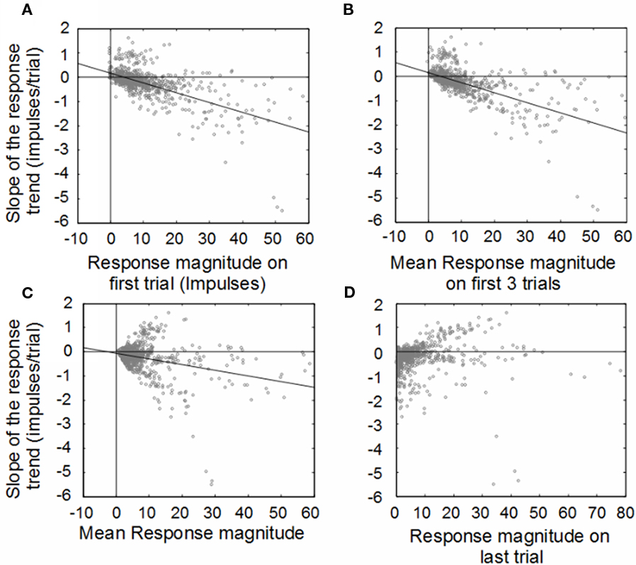
Figure 2. Illustration of correlations between the change (slope) of the response magnitude (y-axis) vs. response magnitudes (x-axis) averaged in different ways. Change is measured by fitting a linear regression to the plot of response magnitude vs. trial number for each neuron. Both the impulse count on the first trial (far left) and the impulse count on the last trial (far right) predict the change (slope) in the response magnitude over the course of the experiment. (A) Weak responses observed on early trials during the experiment tended to potentiate in later trials, while strong responses in early trials tended to habituate in later trials. Averaging the response magnitudes of the first three (B), trials tends to be just a slightly better predictor of the direction and magnitude of the response trend. By comparison, averaging the responses over all the trials (C) is a worse predictor of the direction and magnitude of the response trend, as is examining only the last trial response (D).

Further support for our hypothesis is shown in Figure 3, where the response to a particular stimulus is correlated with the response on its next presentation (2), the presentation after that (3), and the following presentation (4). Note that there are many stimuli presented between each of these presentations. However, if our hypothesis is correct, then we expect to see that, the further away the trial in time, the less predictable the response magnitude will be. On the other hand, if our observations could be explained by simple randomness, then all responses would be equally predictive of each other (i.e., not at all). This was not the case: the more proximate the responses were in time, the better they could be used to predict one another: one-step correlations averaged r² = 0.22, two-step correlations averaged r² = 0.18, and three-step correlations averaged only r² = 0.16.

FIGURE 3

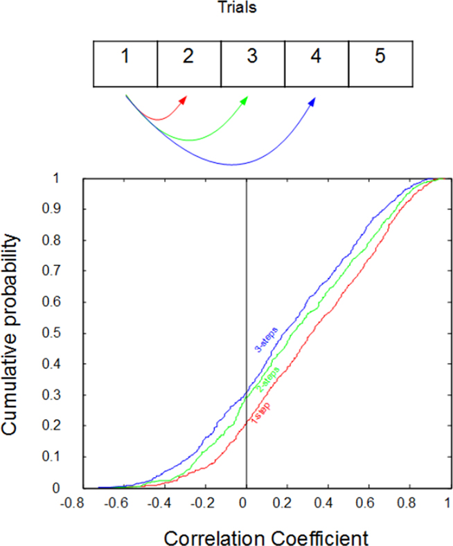
Figure 3. Cumulative distributions of the correlations between the impulse counts on subsequent trials. Despite being randomly interleaved with other types of stimuli, the response to a stimulus on a given trial can typically be predicted from the response on its last exposure (red, “one-step”). However, predictions are progressively worse for responses from two previous exposures (green, “two-steps”), and three previous exposures (blue, “three-steps”). r values are plotted on the x-axis while cumulative probability plotted on the y-axis.

In our final analysis we compared the change in the multisensory responses over time to the changes in the best unisensory responses, which is our traditional method of determining the efficacy of multisensory integration (Figure 4). If the observed response changes were simply random, there would be no correlation in these slopes: the unisensory response might go up while the multisensory response might go down. Instead, we found results consistent with our hypothesis: there was a good correlation (r² = 0.75). These changes were consistent with the principle of inverse effectiveness, and further solidify the conclusion that the neuron studied at the beginning of the experiment has changed state, and so has the benefit of multisensory integration, by its end.

FIGURE 4

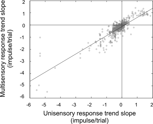
Figure 4. There is a very good correlation between the response trend slopes for multisensory and unisensory responses. Knowing how the unisensory response will change over the course of the experiment is a good predictor of how the multisensory response will change (and vice versa).

Discussion

The Heisenberg uncertainty principle states that certain physical properties, such as position and momentum, cannot be precisely known at a quantum level at the same time because in an effort to study one, one must disrupt the study of another (Wheeler and Zurek, 1983). We know that the nervous system is adaptive, changing its responses to stimuli to which it is exposed, that this plasticity extends well beyond the neonatal period, and that it exists at multiple levels of the neuraxis, including the SC (Yu et al., 2009). The unfortunate consequence is that we cannot study the brain without changing it, though we often take steps to attenuate these changes, for example by increasing interstimulus intervals and presenting different stimuli in a randomly interleaved fashion. The efficacy of these measures is not well-known, but has a great impact on our interpretation of the data that we collect. Here we asked a simple question: in a standard study of multisensory SC neurons exposed to randomly interleaved visual, auditory, and visual–auditory stimulus combinations, did the responses change in a predictable way? The answer was yes, and the consequences are that multisensory integration is different at the beginning of the experiment and at the end, because strong responses habituate and weak responses potentiate.

How well this principle applies to other areas of the brain, especially multisensory areas, is difficult to predict. The SC is engaged in stimulus localization and orientation behaviors (Sparks, 1986; Glimcher and Sparks, 1992; Stein, 1998), and as such, can be thought of as having two goals: the detection of salient (but potentially weak) signals, and the ignoring of events that are not novel (but potentially strong). Our observations suggest how these goals may be balanced. In circumstances in which a relevant event occurs again and again, it would be adaptive to boost the signal when it is weak. In other circumstances, where an irrelevant event repeatedly occurs, it would be adaptive to suppress its signal when it is strong. This plasticity in the neuronal response may be a general feature of the nervous system, and observable in different brain regions with different functions. On the other hand, because other areas of the brain have different functions, they may show different patterns of response changes.

That multisensory and unisensory responses appear to remain correlated throughout these changes is not surprising, and is consistent with the previously described principle of inverse effectiveness (see Stein and Meredith, 1993; Stein et al., 2009). The implications, however, are significant. When we seek to characterize the magnitude of a multisensory interaction, we must take care to appreciate not only how the dependent measure is taken, but when it is taken. Just as the impact of multisensory interactions is greatest at the onset of a response because the magnitude of the response is at its weakest (Rowland and Stein, 2007), multisensory interactions may be bigger at the beginning or end of an experiment, depending on how the neural circuit changes. This means that the neuron might be characterized one way at 2 o’clock, but at 3 o’clock look fundamentally different. Averaging data across an entire experiment may be an issue that requires additional considerations, especially with regard to statistical analyses. However, our findings suggest that a choice must be made between ignoring these changes or embracing them.

Conflict of Interest Statement

The authors declare that the research was conducted in the absence of any commercial or financial relationships that could be construed as a potential conflict of interest.

Acknowledgments

Research was supported by NIH grants EY016716 and NS036916.

References

Alvarado, J. C., Rowland, B. A., Stanford, T. R., and Stein, B. E. (2008). A neural network model of multisensory integration also accounts for unisensory integration in superior colliculus. Brain Res. 1242, 13–23.

Pubmed Abstract | Pubmed Full Text | CrossRef Full Text

Alvarado, J. C., Stanford, T. R., Rowland, B. A., Vaughan, J. W., and Stein, B. E. (2009). Multisensory integration in the superior colliculus requires synergy among corticocollicular inputs. J. Neurosci. 29, 6580–6592.

Pubmed Abstract | Pubmed Full Text | CrossRef Full Text

Bell, A. H., Meredith, M. A., Van Opstal, A. J., and Munoz, D. P. (2005). Crossmodal integration in the primate superior colliculus underlying the preparation and initiation of saccadic eye movements. J. Neurophysiol. 93, 3659–3673.

Pubmed Abstract | Pubmed Full Text | CrossRef Full Text

Burnett, L. R., Stein, B. E., Chaponis, D., and Wallace, M. T. (2004). Superior colliculus lesions preferentially disrupt multisensory orientation. Neuroscience 124, 535–547.

Pubmed Abstract | Pubmed Full Text | CrossRef Full Text

Frens, M. A., and Van Opstal, A. J. (1998). Visual-auditory interactions modulate saccade-related activity in monkey superior colliculus. Brain Res. Bull. 46, 211–224.

Pubmed Abstract | Pubmed Full Text | CrossRef Full Text

Glimcher, P. W., and Sparks, D. L. (1992). Movement selection in advance of action in the superior colliculus. Nature 355, 542–545.

Pubmed Abstract | Pubmed Full Text

Jay, M. F., and Sparks, D. L. (1987). Sensorimotor integration in the primate superior colliculus. I. Motor convergence. J. Neurophysiol. 57, 22–34.

Pubmed Abstract | Pubmed Full Text

Jiang, W., Jiang, H., and Stein, B. E. (2002). Two corticotectal areas facilitate multisensory orientation behavior. J. Cogn. Neurosci. 14, 1240–1255.

Pubmed Abstract | Pubmed Full Text | CrossRef Full Text

King, A. J., and Palmer, A. R. (1985). Integration of visual and auditory information in bimodal neurones in the guinea-pig superior colliculus. Exp. Brain Res. 60, 492–500.

Pubmed Abstract | Pubmed Full Text | CrossRef Full Text

Lee, C., Rohrer, W. H., and Sparks, D. L. (1988). Population coding of saccadic eye movements by neurons in the superior colliculus. Nature 332, 357–360.

Pubmed Abstract | Pubmed Full Text | CrossRef Full Text

McHaffie, J. G., and Stein, B. E. (1983). A chronic headholder minimizing facial obstructions. Brain Res. Bull. 10, 859–860.

Pubmed Abstract | Pubmed Full Text | CrossRef Full Text

Meredith, M. A., Nemitz, J. W., and Stein, B. E. (1987). Determinants of multisensory integration in superior colliculus neurons. I. Temporal factors. J. Neurosci. 7, 3215–3229.

Pubmed Abstract | Pubmed Full Text

Meredith, M. A., and Stein, B. E. (1983). Interactions among converging sensory inputs in the superior colliculus. Science 221, 389–391.

Pubmed Abstract | Pubmed Full Text | CrossRef Full Text

Meredith, M. A., and Stein, B. E. (1986). Visual, auditory, and somatosensory convergence on cells in superior colliculus results in multisensory integration. J. Neurophysiol. 56, 640–662.

Pubmed Abstract | Pubmed Full Text

Meredith, M. A., Wallace, M. T., and Stein, B. E. (1992). Visual, auditory and somatosensory convergence in output neurons of the cat superior colliculus: multisensory properties of the tecto-reticulo- spinal projection. Exp. Brain Res. 88, 181–186.

Pubmed Abstract | Pubmed Full Text | CrossRef Full Text

Peck, C. K., Baro, J. A., and Warder, S. M. (1993). Sensory integration in the deep layers of superior colliculus. Prog. Brain Res. 95, 91–102.

Pubmed Abstract | Pubmed Full Text

Perrault, T. J. Jr., Vaughan, J. W., Stein, B. E., and Wallace, M. T. (2003). Neuron-specific response characteristics predict the magnitude of multisensory integration. J. Neurophysiol. 90, 4022–4026.

Pubmed Abstract | Pubmed Full Text | CrossRef Full Text

Populin, L. C., and Yin, T. C. (2002). Bimodal interactions in the superior colliculus of the behaving cat. J. Neurosci. 22, 2826–2834.

Pubmed Abstract | Pubmed Full Text

Rowland, B. A., Quessy, S., Stanford, T. R., and Stein, B. E. (2007). Multisensory integration shortens physiological response latencies. J. Neurosci. 27, 5879–5884.

Pubmed Abstract | Pubmed Full Text | CrossRef Full Text

Rowland, B. A., and Stein, B. E. (2007). Multisensory integration produces an initial response enhancement. Front. Integr. Neurosci. 1, 4. doi: 10.3389/neuro.07/004.2007

Pubmed Abstract | Pubmed Full Text | CrossRef Full Text

Sparks, D. L. (1986). Translation of sensory signals into commands for control of saccadic eye movements: role of primate superior colliculus. Physiol. Rev. 66, 118–171.

Pubmed Abstract | Pubmed Full Text

Stein, B. E. (1998). Neural mechanisms for synthesizing sensory information and producing adaptive behaviors. Exp. Brain Res. 123, 124–135.

Pubmed Abstract | Pubmed Full Text | CrossRef Full Text

Stein, B. E., and Arigbede, M. O. (1972). Unimodal and multimodal response properties of neurons in the cat’s superior colliculus. Exp. Neurol. 36, 179–196.

Pubmed Abstract | Pubmed Full Text | CrossRef Full Text

Stein, B. E., and Dixon, J. P. (1979). Properties of superior colliculus neurons in the golden hamster. J. Comp. Neurol. 183, 269–284.

Pubmed Abstract | Pubmed Full Text | CrossRef Full Text

Stein, B. E., and Meredith, M. A. (1993). The Merging of the Senses. Cambridge, MA: MIT Press.

Stein, B. E., and Stanford, T. R. (2008). Multisensory integration: current issues from the perspective of the single neuron. Nat. Rev. Neurosci. 9, 255–266.

Pubmed Abstract | Pubmed Full Text | CrossRef Full Text

Stein, B. E., Stanford, T. R., Ramachandran, R., Perrault, T. J. Jr., and Rowland, B. A. (2009). Challenges in quantifying multisensory integration: alternative criteria, models, and inverse effectiveness. Exp. Brain Res. 198, 113–126.

Pubmed Abstract | Pubmed Full Text | CrossRef Full Text

Wallace, M. T., Meredith, M. A., and Stein, B. E. (1993). Converging influences from visual, auditory, and somatosensory cortices onto output neurons of the superior colliculus. J. Neurophysiol. 69, 1797–1809.

Pubmed Abstract | Pubmed Full Text

Wallace, M. T., and Stein, B. E. (2001). Sensory and multisensory responses in the newborn monkey superior colliculus. J. Neurosci. 21, 8886–8894.

Pubmed Abstract | Pubmed Full Text

Wallace, M. T., Wilkinson, L. K., and Stein, B. E. (1996). Representation and integration of multiple sensory inputs in primate superior colliculus. J. Neurophysiol. 76, 1246–1266.

Pubmed Abstract | Pubmed Full Text

Wheeler, J. A., and Zurek, W. H. (1983). Quantum Theory and Measurement. Princeton, NJ: Princeton University Press.

Yu, L., Stein, B. E., and Rowland, B. A. (2009). Adult plasticity in multisensory neurons: short-term experience-dependent changes in the superior colliculus. J. Neurosci. 29, 15910–15922.

Pubmed Abstract | Pubmed Full Text | CrossRef Full Text

Zahar, Y., Reches, A., and Gutfreund, Y. (2009). Multisensory enhancement in the optic tectum of the barn owl: spike count and spike timing. J. Neurophysiol. 101, 2380–2394.

Pubmed Abstract | Pubmed Full Text | CrossRef Full Text