
- Institute of Medical Sciences, Aberdeen Medical School, Aberdeen, UK
Visual cortex analyzes images by first extracting relevant details (e.g., edges) via a large array of specialized detectors. The resulting edge map is then relayed to a processing pipeline, the final goal of which is to attribute meaning to the scene. As this process unfolds, does the global interpretation of the image affect how local feature detectors operate? We characterized the local properties of human edge detectors while we manipulated the extent to which the statistical properties of the surrounding image conformed to those encountered in natural vision. Although some aspects of local processing were unaffected by contextual manipulations, we observed significant alterations in the operating characteristics of the detector which were solely attributable to a higher-level semantic interpretation of the scene, unrelated to lower-level aspects of image statistics. Our results suggest that it may be inaccurate to regard early feature detectors as operating outside the domain of higher-level vision; although there is validity in this approach, a full understanding of their properties requires the inclusion of knowledge-based effects specific to the statistical regularities found in the natural environment.
1 Introduction
Natural scenes are characterized by highly structured statistical properties (Ruderman and Bialek, 1994; Mante et al., 2005; Frazor and Geisler, 2006). The fundamental question of whether these properties are reflected in the response characteristics of sensory systems has been actively debated in recent years (Felsen and Dan, 2005; Rust and Movshon, 2005). Although potentially relevant phenomena (e.g., alterations of receptive field structure) are still under investigation (Ringach et al., 2002; Smyth et al., 2003; David et al., 2004; Touryan et al., 2005), there is consensus over the notion that the selectivity of sensory neurons is matched to the statistics of the natural environment (Rieke et al., 1995; Vinje and Gallant, 2002; Felsen et al., 2005; Woolley et al., 2005; Yu et al., 2005). Because human vision is supported by this neuronal machinery, we expect perceptual processing to show some degree of specificity for the image regularities that characterize natural scenes (e.g., the tendency for edges to fall along contours; Geisler, 2008). It is clear that the human ability to process natural images depends on the integrity of local statistical properties (Piotrowski and Campbell, 1982; Bex et al., 2007, 2009) and many aspects of pattern vision, such as center–surround interactions (Yu and Levi, 2000; Paradiso et al., 2006) or contrast gain control (Bex et al., 2007), are able to account for a large part of how visual sensitivity depends on specific image manipulations of natural scenes (Geisler et al., 2001; Bex et al., 2007).
An altogether different question is whether the semantic interpretation of the image can impact how local sensors operate in the human observer; answering this question relies on the ability to interfere with image interpretation while at the same time leaving local statistics unaffected. One of the few manipulations that can achieve this goal is image inversion (Valentine, 1988): the interpretation of natural scenes can differ dramatically when viewed upside-down (Thompson and Thatcher, 1980), a result that poses serious challenges for classification algorithms based on low-level statistical properties (see Figure 7 in Torralba and Oliva, 2003 for an example). Image inversion therefore represents a powerful tool for gauging the impact of semantic processing on visual sensitivity (Valentine, 1988; Yovel and Kanwisher, 2005), but so far it has been exploited in relation to tasks and experimental protocols that were not designed to target the properties of local sensors in human vision (Yin, 1969; Wright and Roberts, 1996).
Our goal was to combine low-level characterizations of human feature detectors afforded by behavioral reverse correlation (Ahumada, 2002; Neri and Levi, 2006) with the higher-level manipulation of image semantics introduced by inversion (Valentine, 1988). To this end we embedded artificially generated edges within natural scenes and perturbed their local properties via a controlled noise source, allowing us to deploy well-established techniques for characterizing human perceptual filters to the domain of natural image statistics. We chose this methodology because, as we demonstrate by combining data from several experimental manipulations (Figure 15), it can provide information that is not made available by more classic performance metrics such as sensitivity (Neri and Levi, 2007; Nagai et al., 2008; Dobres and Seitz, 2010). We found that the shape of the perceptual filters was affected by image inversion in specific and reproducible ways, delivering a dynamic picture of how low-level human sensors reshape their response properties under the instruction of higher-level image analysis.
2 Materials And Methods
2.1 Natural Image Database
We initially obtained five databases from the internet. Four were directly downloaded from http://cvcl.mit.edu/database.htm [at the time of downloading they contained 330 ± 50 (mean ± SD across datasets) images each]; the category labels assigned by the database creators (see Oliva and Torralba, 2001) were “forest,” “mountain,” “highway,” and “tall building.” The fifth database consisted of 206 face images from the Stirling database (http://pics.psych.stir.ac.uk/) selected for frontal and 3/4 view, which we resized to match the pixel size of the other databases (256 × 256). We therefore started with a total of ∼1.5 K images. Of these we selected 240 (roughly 1 out of 6) using an entirely automated software procedure (no pick-and-choose human intervention). We first acquired each image as grayscale, rescaled intensity to range between 0 and 1 and applied a smooth circular window so that the outer edge of the image (5% of diameter) was tapered to background gray (see Figure 1A). We refer to this windowed image as the “upright natural image.” We then applied a Sobel filter of dimension equal to ∼15% image size to identify the location of peak edge content. Subsequent to edge detection we applied a broad low-pass Gaussian filter (SD equal to half image size), rescaled intensity to range between 0 and 1 and set all image values above 1/2 to bright, all those below to dark. We refer to this image as the “blob-like” image. We then created an image of size equal to the Sobel filter containing an oriented sharp edge, centered it on the previously determined location of peak edge content, and matched its orientation to the local structure of the “blob-like” image by minimizing square error (MSE). The resulting MSE value was used as primary index of how well that particular image was suited to the purpose of our experiments. We analyzed all images using the procedure just described and only retained the top 40 for each of the 4 non-face databases (those with smallest MSE value within their database), 80 for the face database. For each of these images we generated phase-only and power-only versions by Fourier transforming them and substituting either their power spectrum or their phase spectrum with that of an image containing white noise (this procedure was carried out only once for each image and the resulting images were kept fixed throughout the experiments, i.e., we did not generate new power-only and phase-only images on every trial to avoid the potential introduction of an additional external noise source). Finally, all images were rescaled to have the same contrast energy when projected onto the monitor; they spanned a range between 4 and 60 cd/m2 on a gray background of 32 cd/m2.
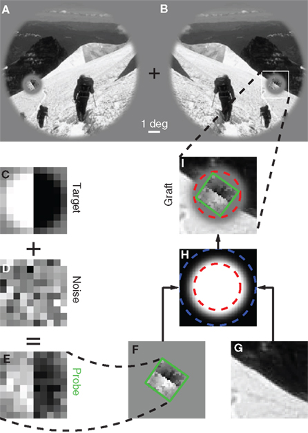
Figure 1. Stimulus design and experimental protocol. Observers were asked to select one of two images (A versus B) that appeared to the sides of a central fixation cross. The target image [(B) in this example] contained a grafted edge (indicated by the white square) that was aligned with the local characteristics of the picture (the mountain ridge in this example), the non-target image (A) contained a similar graft but oriented orthogonally to the local structure of the picture. We created the graft by smoothly inserting a probe (green outline) into the natural scene. The probe (E) consisted of a target edge (C) superimposed onto Gaussian noise (D); it was rotated (F) to match the local structure of the picture (G) and then inserted via a smooth envelope (H). The envelope was designed so that the probe would be isolated from the natural scene within the resulting graft (I). See Section 2.2 for more details.
2.2 Probe Design and Insertion
Please refer to Figure 1. The probe (Figure 1E) consisted of an oriented edge (Figure 1C) added to a 2D sample of Gaussian noise (Figure 1D). It was smoothly inserted into the local region of the natural image (Figure 1G) identified by the automated edge-detection procedure detailed above, at the orientation corresponding to the image MSE value. Insertion was performed via the smooth circular window shown in Figure 1H, where the region within the red dashed circle was set to 1, the region outside the blue dashed circle to 0, the transition region between the red and the blue circles to a cumulative Gaussian ramp. The probe was centered on peak edge and optimally oriented to obtain Figure 1F. The images in Figures 1F,G were then averaged after weighting by the insertion window: Figure 1F was weighted by the image in Figure 1H, while Figure 1G was weighted by 1 minus the image in Figure 1H. The resulting graft is shown in Figure 1I. The insertion was specifically designed so that the region occupied by the probe (outlined in green) was inside the red dashed circle, meaning that no contamination from the natural image was present within the probe. The statistics of the probe was therefore under direct experimental control. The target stimulus was created by inserting the probe at the correctly aligned orientation (Figure 1B); the non-target stimulus by making the probe orthogonal (in the specific way shown by the small icons to the left of Figures 2A,C) prior to insertion (Figure 1A).
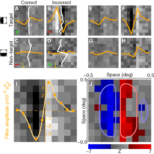
Figure 2. Procedure for deriving the perceptual filter from classified noise. Data from aggregate observer (>180 K trials). (A–D) Show average noise images from target (A,B) or non-target (C,D) probes on correct (A,C) or incorrect trials (B,D). Yellow traces show marginal averages taken vertically across the image, white traces horizontally. Before combining all four images into 1, some were summed [green + signs in (A,D)] and others were subtracted [red − signs in (B,C)] as well as transposed [yellow ⊥ symbol in (C,D)], to obtain the four images shown in (E–H) (see Section 2). The combined image is plotted in I (yellow trace shows marginal average in units of external noise variance  ), and a Z score map of this image is shown in (J) [colored pixels refer to Z| > 2]. The smooth outlines in (J) show contour lines at 1/3 (light red) and −1/3 (light blue) of peak value for the pseudo-Gabor fit (see Section 2.6).
2.3 Stimulus Presentation and Psychophysical Task
The overall stimulus consisted of two simultaneously presented images (duration 300 ms), one to the left and one to the right of fixation (Figures 1A,B). On every trial we randomly selected an image from the database and created both target and non-target stimuli from the same image, but using independent noise samples for the two (randomly generated on every trial). We then presented the target on the left and the non-target on the right, or vice versa (randomly selected on every trial). Whichever was presented to the right was mirror-imaged around vertical, so that the probes were symmetrically placed with respect to fixation (see Figures 1A,B). At the adopted viewing distance of 57 cm the diameter of each stimulus was 12° (centered at 7.3° from fixation) and the probe measured 1 deg × 1 deg. On precue trials the main stimulus just described was preceded by a spatial cue (duration 100 ms) consisting of two Gaussian blobs (matched to probe size) that co-localized with target and non-target probes (see Figure 6A); the interval between cue and main stimulus was uniformly distributed between 150 and 300 ms. On postcue trials the same cue was presented but it followed the main stimulus (after the same interval detailed for precue). Observers were required to select the stimulus containing the target (by pressing one of two buttons to indicate either left or right of fixation); their response was followed by trial-by-trial feedback (correct/incorrect) and initiated the next trial after a random delay uniformly distributed between 200 and 400 ms. At the end of each block (100 trials) observers were provided with a summary of their overall performance (percentage of correct responses on the last block as well as across all blocks) and the total number of trials collected to that point. We tested eight naive observers with different levels of experience in performing psychophysical tasks. The intensity of the target signal (maximum value of image in Figure 1C) was adjusted individually following preliminary estimation of threshold point via a two-down one-up staircase procedure; it was 1.27 ± 0.18 (average ±1 SD across observers) in units of SD of the pixel Gaussian noise source (Figure 1D) which was set to 3 cd/m2. All conditions were mixed within the same block except for the phase-only manipulation, meaning that we ran two types of block: for type 1 each trial presented an image randomly selected from the entire dataset and could be precued or postcued (equiprobable at 1/2), upright or inverted, or blob-like (equiprobable at 1/3); for type 2 each trial presented a phase-only image randomly selected from the entire dataset and could be precued or postcued (equiprobable at 1/2), upright or inverted (equiprobable at 1/2). We collected 22.6 ± 8.8 K trials per observer (this figure includes half the trials from double-pass experiments, see section below). Overall we collected slightly more trials (∼22%) for each of the three main image types (e.g., natural upright) as opposed to each of the two phase-only image types. We collected 238 ± 74 trials per observer for the power-only condition (Figure 11).
2.4 Double-Pass Experiments and Internal Noise
We estimated internal noise (y axis in Figure 3D) via a double-pass methodology in which the same set of stimuli is presented twice (Burgess and Colborne, 1988; please refer to Neri, 2010a for details regarding this well-established technique). Double-pass experiments consisted of 100-trial blocks (like in the main experiment). Observers were not aware of any difference with respect to blocks for the main experiment. In double-pass blocks, the second half of the block (last 50 trials) showed the same stimuli presented during the first 50 trials, but in randomly permuted order. We collected an average of 1.6 ± 0.8 K trials per observer. Half of these (the first 50 trials of each block) were extracted and combined with trials from the main experiment.
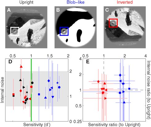
Figure 3. Sensitivity and internal noise for upright natural (A), blob-like (B) and inverted images (C); color-coding is black, blue and red respectively. (D) Plots d′ on the x axis versus internal noise on the y axis (see Section 2.4 for details on how the latter was estimated). Gray shading shows internal noise range expected from previous studies (Neri, 2010a); green vertical line shows the desired d′ target value of 1 (Murray et al., 2002). (E) Plots ratios between d′ for blob-like and d′ for upright natural images (blue) on the x axis, versus ratios between internal noise for blob-like and internal noise for natural images on the y axis. Red symbols plot the same but for inverted instead of blob-like images. Dashed lines indicate unity ratios. Each symbol refers to a different observer. Error bars show ±1 SEM.
2.5 Computation of Perceptual Filters
Each noise sample can be denoted by the matrix N[q,z], i.e., the 2D noise image that was added to the target probe (q = 1) or the non-target probe (q = 0) on a trial to which the observer responded correctly (z = 1) or incorrectly (z = 0). The four panels in Figures 2A–D refer to the four possible ways of classifying a given noise sample: q = 1 and z = 1 (A), q = 1 and z = 0 (B), q = 0 and z = 1 (C), q = 0 and z = 0 (D). The standard formula for combining averages from the four classes into a perceptual filter P is (Ahumada, 2002): P = 〈N[1,1]〉 − 〈N[1,0]〉 − 〈N[0,1]〉 + 〈N[0,0]〉 where 〈〉 is average across trials of the indexed type; this combination rule is reflected by the green + and red − signs in Figures 2A–D. For the specific application of interest it was necessary to modify this rule slightly as follows:  where T is transpose, indicated by the yellow ⊥ symbol in Figures 2C,D. This modification was motivated by both logical considerations (see below) and by computational modeling (Figure 14). Close inspection of 〈N[1,1]〉 in Figure 2A, which is the 2AFC equivalent of a “hit” classified image, demonstrates that (as expected) it resembles the target edge (icon plotted to the far left): it modulates along the horizontal axis from dark to bright (see marginal orange trace in Figure 2A), but not along the vertical axis (white trace). Similarly 〈N[1,0]〉 in Figure 2B, which is the equivalent of a “miss” image, conforms to the expectation of an inverted image of the target edge. For both Figures 2A,B the standard rule of adding the former and subtracting the latter is therefore applicable. The standard rule, however, was primarily formulated for designs in which the non-target is a scaled image of the target (Ahumada, 2002; Murray et al., 2002). The non-target we used in this study (icon plotted to the far left) was oriented orthogonal to the target, a difference that cannot be accommodated by scaling (with or without sign inversion). For this reason 〈N[0,0]〉 in Figure 2D, which is the equivalent of a “false alarm” image, is not a scaled version of Figure 2A as is normally expected (Ahumada, 2002; Neri, 2010b) but retains the orientation of the non-target signal that was embedded within this noise probe; it is therefore better thought of as a “miss” image where it is the non-target (rather than the target) that was missed. When viewed this way, it becomes clear why it was necessary to re-align its orientation to the target via transpose before combining it with Figures 2A,B. A similar procedure was necessary for 〈N[0,1]〉 in Figure 2C, the equivalent of a “correct rejection” image but more appropriately viewed as a “hit” image for the non-target; because the corresponding noise probes contained a non-target signal the edge-related modulation (dark/bright) is only present along the vertical axis (see white marginal trace) and not the horizontal (orange trace), requiring orientation re-alignment in addition to the sign inversion prescribed by the original rule (Ahumada, 2002). Following these simple transformations the four images in Figures 2A–D are re-aligned to the same reference as shown in Figures 2E–H, and can then be combined into a final perceptual filter image (Figure 2I) that shows a clear structure resembling the target edge. Throughout the article we present these images as Z score maps with overlaid fitting from a pseudo-Gabor function (see section below for specifics on this fitting procedure), shown in Figure 2J. Together with the rationale just described, we also confirmed that the chosen combination rule is sensible via simulations (see Figures 14T–Σ and related text in the Section 3). For some analyses involving parcellation of the dataset, in particular precue/postcue (Figures 7A,B and 10C,D) and scenes/faces (Figure 13), we smoothed the filter estimates in order to compensate for dataset reduction; smoothing was achieved via Wiener denoising (Matlab function wiener2 with default parameter settings).
2.6 Scalar Metrics for Assessing Filter Structure
Oddity index (x axis in Figure 5A) was computed as log[Φ(P odd)/Φ(P even)] where Φ is mean of squares ( across d elements ai,j of matrix A).
  and
and  (see Bracewell, 1965), where
  and
and  is the mean value across the entire filter, i.e.,
  (we subtracted the DC component in this way to ensure that simple baseline shifts would not bias our shape estimate), and P* is the mirror image of P around the vertical midline. SNR (y axis in Figure 5A) was computed as
  (see Murray et al., 2002; Neri, 2010b) where n[1] is the number of correct trials, n[0] is the number of incorrect trials and w is the variance of the external noise source. Target similarity (x axis in Figure 5B) was simply the signed correlation r2 between P and T (element-by-element) where T is the target image (Figure 1C). Target-weighted energy (y axis in Figure 5B) was Φ(P ○ T) where ○ is Hadamard (i.e., element-by-element) product. The pseudo-Gabor wavelet we used for the fitting results in Figure 5D was G = |T| ○ C where each element ci,j of the matrix C was defined by ci,j = cos(2πω(xj + φ)) (no dependence on i) and the vector x (containing elements xj) ranged from −1 to 1. This wavelet is a sinusoidal grating modulated by the target envelope rather than a Gaussian; we adopted this formulation to minimize the number of free parameters for fitting (we can drop SD of the Gaussian envelope). For the same reason, before fitting we enforced matched energy between the wavelet and the perceptual filter, i.e., Φ(G) = Φ(P) (allowing us to drop the parameter of overall amplitude). There were two free parameters left: the frequency of the sinusoidal carrier ω expressed in units of cycles per filter width, which is equivalent to cycles per degree because the width of the probe was 1 deg; and the phase of the sinusoidal carrier φ expressed in units of fraction of a cycle (e.g., when equal to 1/4 the cosine function is a sine function, see green icon above green vertical line in Figure 5D). Fitting relied on the Matlab routine nlinfit.
2.7 Combined Index for Change in Filter Shape
Our goal for Figure 15 was to plot changes in sensitivity versus changes in filter shape using comparable units. We could not use differences (e.g., oddity for blob-like minus oddity for natural) because the two metrics would be expressed in their own units, so we used log-ratios. For filter shape we adopted a composite index combining both oddity and target similarity by taking the log of the mean between exp(o1)/exp(o2) and t1/t2 where o is oddity, t is target similarity and numerical subscripts refer to the two conditions being compared [by applying exp(.) we effectively used oddity as Φ(P odd)/Φ(P even) to preserve positive quantities before taking ratios; this was not necessary for target similarity because all values were already positive]. The change in sensitivity plotted on the x axis in Figure 15 was simply the logged d′ ratio. Low-level comparisons included all manipulations except image inversion, and each black symbol in Figure 15 refers to one low-level comparison for one observer. For example if we compared blob-like versus upright natural image, the x axis would plot the sensitivity ratios already plotted on the x axis in Figure 3E (logged) while the y axis would plot the composite index detailed above from the oddity and target similarity values plotted in Figure 5 for blue versus black symbols (log-ratio between blob-like and upright natural). More specifically, black symbols in Figure 15 plot the following comparisons: blob-like versus upright natural, blob-like versus inverted natural, upright phase-only versus upright natural, inverted phase-only versus inverted natural, precue versus postcue for upright natural, precue versus postcue for inverted natural, precue versus postcue for blob-like, precue versus postcue for upright phase-only, precue versus postcue for inverted phase-only, upright natural scenes versus faces, inverted natural scenes versus faces, upright phase-only scenes versus faces, inverted phase-only scenes versus faces. Higher-level comparisons (red symbols) were: upright versus inverted natural on precue trials, upright versus inverted natural on postcue trials, upright versus inverted phase-only on precue trials, upright versus inverted phase-only on postcue trials. The rationale behind these selections was to include as many comparisons as possible without subdividing the dataset into excessively small chunks.
2.8 Modeling
Please refer to Figure 14. The output of model in panel A is rA = R • S where S is the probe image (e.g., Figure 1E), • is Frobenius inner product (A • B = Σi,j ai,jbi,j), and R = C as defined above with ω = 1 and φ = 1/4 (see grating in Figure 14A). The output of the model in panel B is the same but squared, i.e.,  The output of the model in panel C is
  where the output
  is the same as rB except the underlying template R is oriented orthogonally (see Figure 14C). Each model generates an output value r[1] in response to the target stimulus and an output value r[0] in response to the non-target stimulus; the model then responds correctly if r[1] > r[0], incorrectly otherwise. The simulated filters in Figure 14 were obtained by applying the same analysis to the model that was used with the human observers. We set target intensity to the value (1/4) that corresponded to model d′ ∼ 1.
3 Results
We mapped local edge detectors via noise image classification (Ahumada, 2002), a psychophysical variant of reverse correlation. In this method a controlled noisy perturbation is applied to a local target edge, which we embedded within a structured image (Figure 1B). Observers saw two such images on every trial, and were asked to select the image containing a meaningfully embedded “target” edge (Figure 1B) as opposed to an orthogonal “non-target” edge which did not fit its surround (Figure 1A). By studying how individual noise samples affected the response generated by observers on specific trials we were able to derive perceptual filters analogous to the neuronal receptive fields measured in the electrophysiological literature (Neri and Levi, 2006); an example is shown in Figure 2I (with corresponding Z map in Figure 2J) where the edge-like structure of the filter is clearly visible and in conformity with its expected function of detecting the target edge. This filter was obtained by combining noise averages from both target/non-target probes and correct/incorrect trials, separately shown in Figures 2A–D; prior to adding them together, they were rotated and/or sign-inverted to bring them into alignment with the target edge as shown in Figures 2E–H (see Sections 2.5 and 3.7).
The question of whether sensory filters alter their characteristics in response to natural statistics has received considerable attention in recent years (Kayser et al., 2004; Felsen and Dan, 2005; Rust and Movshon, 2005; Geisler, 2008), but it has proven more challenging than anticipated due to the difficulty of applying reverse correlation to non-white inputs (Smyth et al., 2003; Sharpee et al., 2008). Our approach completely bypasses this issue by retaining a white noise probe (see Section 2 and Figure 1D), the local statistics of which is isolated from the natural image via an insertion envelope that does not allow for spatial overlap between probe and image (Figure 1H). The final graft consists of a region containing only the probe, surrounded by a region of smooth transition into the natural image (Figure 1I). By adopting this specific design we are in a position to apply established methods for psychophysical reverse correlation with white inputs (Ahumada, 2002; Neri, 2010b), eliminating the concern for artifacts having to do with the statistics of the images per se (Smyth et al., 2003; Sharpee et al., 2008). At the same time we can gauge the effect of image statistics on our filter estimates by embedding the probe within images of different character (e.g., natural versus artificial) and assigning a task that requires observers to integrate both probe and image context to perform above chance (see immediately below). Because the statistical properties of the probe are identical across changes in image types, any resulting alteration in the estimated perceptual filter must be attributed to the statistics of the surrounding image and not to possible artifacts of the estimation technique.
An additional critical feature of our experimental design was that target and non-target stimuli were statistically indistinguishable when viewed out of context: if we imagine removing the image regions outside the two inserts in Figures 1A,B, observers would see an oriented edge on one side of fixation and a differently oriented edge on the other side, with no way of knowing which one to choose. Similarly, no useful information was provided by context alone: if we imagine removing the image regions within the inserts in Figures 1A,B, observers would see a natural scene with a hole on one side of fixation and its mirror image on the other side, with no indication that one should be preferred over the other. The task of choosing the image containing a registered target probe could only be performed by integrating both context and probe in a meaningful fashion.
3.1 Performance Metrics
The black symbols in Figure 3D show sensitivity (d′) on the x axis versus internal noise on the y axis for detecting edges within natural scenes similar to the one shown in Figure 3A. The term internal noise refers to a source of response variability that is intrinsic to the observer, as opposed to the response variability induced by the external noise source in the stimulus; the reader is referred to Neri (2010a) for a detailed review of this concept and its application to human sensory processing. Internal noise was independently estimated using a standard approach termed double-pass (see Section 2.4). Across our sample d′ was near 1 (mean 1.00 ± 0.13 SD across observers), as targeted by our protocol (see Section 2) and as recommended for the application of psychophysical reverse correlation (Murray et al., 2002). Internal noise was in the range 0.6–2 (indicated by gray shading in Figure 3D), well within previous estimates (Neri, 2010a). Overall it is clear that observers understood the task and adopted a stable consistent strategy to perform it (reasonable internal noise).
We then applied two manipulations to the region outside the target edge. The first manipulation consisted of replacing the natural image with a blob-like version that retained some coarse features from the original image (see Section 2); an example is shown in Figure 3B. The purpose of this manipulation was to test the effect of replacing the natural image with one that resembles simple laboratory stimuli, while at the same time retaining task-relevant aspects of the original image (i.e., most evident edge structure) so as to allow reasonable comparisons. The blue symbols in Figure 3D show that this manipulation produced a marked increase in sensitivity (blue symbols lie to the right of black symbols, paired t-test returns p < 10−8) but no change in the intensity of internal noise (p = 0.49). Both effects can be verified more readily by replotting the data in terms of ratios between values for the blob-like images and values for the natural images, as shown by the blue symbols in Figure 3E: sensitivity ratios (x axis) are >1 (blue points lie to the right of vertical dashed line at p < 10−6) while internal noise ratios (y axis) are near 1 (blue points fall on horizontal dashed line at p = 0.41). This result is consistent with electrophysiological reports that the response of V1 neurons is suppressed more effectively by surround stimuli with natural as opposed to scrambled/featureless characteristics (Guo et al., 2005; MacEvoy et al., 2008). The lack of any significant change in internal noise is perhaps more surprising in light of existing electrophysiological literature (Vinje and Gallant, 2002; Kayser et al., 2003; Yu et al., 2005; Tolhurst et al., 2009), but it is known that response variability in human observers is dominated by a late decisional noise source with remarkably stable characteristics against large variations in stimulus properties, task specifications, and even sensory modality (Neri, 2010a).
The second manipulation consisted of inverting the entire display upside-down (Figure 3C). Differently from the blob-like manipulation detailed above, stimulus inversion has virtually no effect on commonly studied statistical properties of the image (e.g., Fourier power, see Torralba and Oliva, 2003). As shown by the red symbols in Figure 3D this manipulation had little or no effect on both sensitivity and internal noise (compare with blue symbols). We can verify this result more transparently in Figure 3E, which shows that sensitivity ratios between upright and upside-down conditions are near 1 (red points fall on vertical dashed line at p = 0.57) and that the same applies to internal noise ratios (red points fall on horizontal dashed line at p = 0.84). The latter result is consistent with previous reports (Gaspar et al., 2008).
3.2 Structure of the Perceptual Filters and Its Dependence on Context
Figures 4D–F show perceptual filters derived separately for the three different conditions detailed above: natural image (A), blob-like image (B), and inverted natural image (C). As expected, they all resemble to some extent the target edge that observers were asked to detect. However they also appear to differ in some respects from one condition to another: the perceptual filter derived from trials showing inverted natural images (F) contains additional ripples at the outer edges, which are not present in the perceptual filter derived from upright natural images (D), and its central zero-crossing is misplaced with respect to the vertical line defined by the target edge (white vertical dashed line).
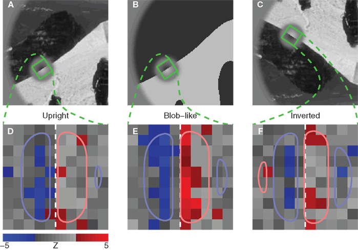
Figure 4. Perceptual filters (D–F) for upright natural (A), blob-like (B) and inverted images (C). Plotted to the same conventions of Figure 2J. Dashed vertical lines indicate target edge location.
It is not possible to draw firm conclusions from a qualitative inspection of aggregate data like that shown in Figure 4, nor is it possible to inspect perceptual filters for individual observers (see Figure A1 in Appendix) as they show significant variability [expected from previous work (Meese et al., 2005; Neri, 2010b)] and present the same challenge of only allowing primarily qualitative considerations. We therefore performed additional analyses that captured relevant aspects of the perceptual filters (see below), and quantified each aspect using a single value for each observer. The data could then be subjected to simple population statistics in the form of two-tailed t-tests and confirm or reject specific hypotheses about the overall shape of the filters. Our conclusions are therefore based on individual observer data, not on the aggregate observer (which is used solely for visualization purposes); this distinction is important because there is no generally accepted procedure for generating an average filter from individual images for different observers (see Neri and Levi, 2008 for a detailed discussion of this issue). We arbitrarily adopt a notional threshold of p = 0.05 for statistical significance; reducing this threshold would translate into an overly conservative test in favor of the null hypothesis, which is problematic for the analysis we present below because our interest is not in confirming or rejecting the null hypothesis, but rather in showing that the same dataset can either favor it or not depending on the manipulation we have chosen to apply before collecting the data. We choose an empirical strategy to test for robustness of the results: we collect more data in different conditions and show that the same result is obtained from independent datasets (see Section 4).
We adopted three metrics to capture the shape of the perceptual filters (detailed in Section 2.6). The first metric measures “oddity” of the filter around the midline by taking the log-ratio between odd and even energy along the direction orthogonal to the edge. The target edge itself is infinitely odd; had it been a bar in the middle, it would have been infinitely even. For empirical estimates like those shown in Figure 4 the oddity metric never reaches infinity due to the inevitable presence of measurement noise; when the estimated surface contains noise and nothing else, the metric returns 0. This specific outcome, i.e., a featureless filter containing modulations that solely reflect the properties of the external noise source in the stimulus, is the natural null hypothesis for statistical testing. Figure 5A plots oddity on the x axis for the three main conditions we have considered so far (color-coding as before). Perceptual filters for upright natural images are significantly odd (black points lie to the right of vertical orange line at p < 0.03 on a two-tailed t-test), and so are those for blob-like images (blue points lie to the right of vertical orange line at p < 0.01). Perceptual filters for inverted natural images, on the other hand, present a roughly equal degree of oddness and evenness (red points lie on the vertical orange line at p = 0.82).
There is a potentially trivial explanation for the lack of oddity in the perceptual filters from inverted images: they may simply contain noise. As mentioned above, a surface generated from noise (where for example each pixel value comes from a normal distribution) will on average return an oddity value of 0. If our method for estimating perceptual filters failed for the inverted condition, but not for the upright condition, then we would expect the observed difference in oddity between the two conditions. We can rule out this interpretation by computing the SNR of individual perceptual filters (Murray et al., 2002; Neri, 2010b); for the SNR index we used (see Section 2.6) SNR = 0 for the hull hypothesis of a filter containing solely noise. The SNR index is constructed in relation to this null hypothesis, so it does not assume any underlying model (e.g., linear observer model): it estimates the departure of perceptual filters from the null hypothesis of full decoupling between stimuli and response, regardless of the characteristics of the underlying process. We plot this quantity on the y axis in Figure 5A to demonstrate that SNR > 0 for all three conditions (points lie above horizontal dashed line at p < 0.02 for black, p < 0.003 for blue and p < 0.003 for red). We conclude from this analysis that the measured lack of oddity for the perceptual filters from inverted images is not a consequence of lack of structure: the inverted perceptual filters contain at least as much structure (assessed by SNR) as the upright perceptual filters (in fact the average SNR value for the inverted condition at 0.23 ± 0.14 was larger than for the upright condition at 0.16 ± 0.14); yet this structure is equally odd and even for the former, mostly odd for the latter. A somewhat related concern is that observers may have been “put off” by inverted images and mostly ignored them; this interpretation is inapplicable because observers performed equally well with upright and inverted images (Figures 3D,E). Finally, the SNR analysis indicates that the tendency for oddity to be larger with blob-like images (blue cluster is shifted to the right of black cluster) may simply result from the concomitantly larger SNR values associated with the blob-like manipulation (blue cluster is shifted upwards of black cluster).
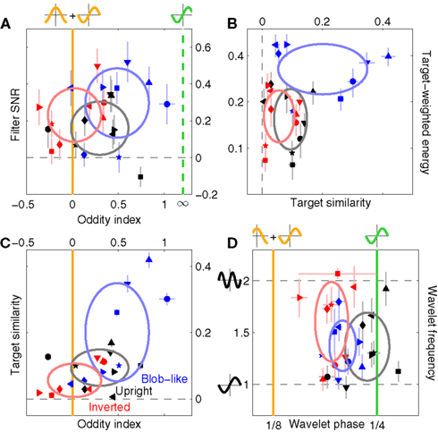
Figure 5. Filter shape metrics. (A) Plots filter oddity (log-ratio between odd and even energy) on the x axis, versus filter signal-to-noise ratio (SNR) on the y axis (see Section 2.6 for definitions of these quantities). Vertical orange line indicates oddity index of 0, corresponding to equal odd and even content (see orange cosine + sine icon above line). Vertical green line indicates oddity index of 8, corresponding to a noiseless odd function (see green sine icon above line). Horizontal dashed line indicates filter SNR of 0, corresponding to noise baseline (filter containing only measurement noise). Ovals are centered on corresponding mean values and radius equals SD. (B) Plots target similarity (correlation between perceptual filter and target shape) on the x axis, versus energy of target-weighted filter on the y axis (see Section 2.6). (C) Plots oddity [from x axis in (A)] on the x axis versus target similarity [from x axis in (B)] on the y axis. (D) Plots phase (x axis) and frequency (y axis) parameters for the pseudo-Gabor fit (see Section 2.6). Orange and green lines indicate phase values somewhat connected to the lines in (A), although oddity and phase are conceptually different quantities (see Section 2). Horizontal dashed lines indicate carrier frequencies of 1 and 2 cycles per degree (see sinusoidal icons to the left of y axis).
The second metric was designed to assess the similarity between the perceptual filter and the target signal; it simply consisted of the point-by-point correlation between the two surfaces (see Section 2.6). Because the target signal was odd, this similarity index bears some relationship to the oddity index: a largely odd perceptual filter is expected to return a high similarity index as well as a high oddity index. We therefore expect that the pattern we measured for oddity in Figure 5A would be roughly preserved by target similarity. The latter quantity is plotted on the x axis in Figure 5B; as expected from the oddity index analysis, perceptual filters for upright perceptual filters show larger similarity values than the corresponding filters from inverted images (black points lie to the right of red points at p < 0.04 on a paired t-test), despite both being greater than 0 (at p < 0.02) meaning that both contained structure. Furthermore, there was no difference in target-weighted energy (p = 0.85) which we document on the y axis. This quantity measures filter energy after weighing by the target shape (see Section 2) and is largest for blob-like filters (blue points fall above black points at p < 0.001).
Before detailing results from the third metric, we emphasize that the two metrics considered so far do not involve any fitting procedure: they return a non-parametric estimate of overall filter shape. The oddity index is particularly useful because it involves minimal assumptions and is desirable for a number of theoretical reasons. First, luminance-defined image features are commonly classified into edges and lines: edges are odd functions, lines are even functions (Marr, 1982). This distinction derives from an established body of biologically motivated image processing literature (Morrone and Burr, 1988; Morgan, 2010). Second, the even/odd distinction has informed psychophysical (Field and Nachmias, 1984; Bennett and Banks, 1991) as well as electrophysiological work (Pollen and Ronner, 1981) and has led some investigators to propose that only even and odd phases are initially encoded at the level of both perceptual sensors and single neurons (Burr et al., 1989). Third, the even/odd characterization is arguably the most general description for an arbitrary function and plays a central role in Fourier-based analysis (Bracewell, 1965), which is directly relevant to signal processing in human vision (Graham, 1989).
For the reasons detailed above we favor the oddity and the target-similarity metrics over the third metric, which assumes a specific shape for the perceptual filter and involves a fitting procedure to optimize the parameterization of the assumed model. Besides the undesirable feature of relying on specific assumptions, this approach is very sensitive to measurement noise (see also Smyth et al., 2003 for similar issues) and is therefore less robust; we implemented it nonetheless because it can be useful for visualization purposes (e.g., contour lines in Figure 4). We report results from this analysis in Figure 5D, where we fitted a wavelet similar to a 2D Gabor to the perceptual filters (see Section 2.6 and Figures 4D–F for examples); the phase of the cosine carrier function is reported on the x axis, its frequency on the y axis. Because these two quantities are not defined for a filter containing only noise, we tailored statistical testing to the next natural null hypothesis of the filter reflecting the target shape (phase value of 1/4). As expected from the preceding analysis based on oddity (Figure 5A) and target similarity (Figure 5B), perceptual filters from upright natural images cluster around the phase value of 1/4 (% of cycle) corresponding to an odd wavelet (black points fall on vertical green line at p = 0.25), while those from inverted images show significantly smaller values than the odd prediction (red points fall to the left of the vertical green line at p < 0.0002) and are shifted toward the odd + even value of 1/8 (vertical orange line). Blob-like filters fall in between, which is perhaps unexpected from the two analyses detailed previously. Although there appeared to be a slight tendency for inverted filters to show higher wavelet frequencies (the red cluster is somewhat shifted upwards compared to the black cluster) this effect was not significant (p = 0.23).
Figure 5C combines the two non-parametric indices for assessing filter shape, the oddity index on the x axis versus the target similarity index on the y axis (same values as x axes in Figures 5A,B). The pattern emphasized by this plot is one where clusters shift upward to the right as we consider perceptual filters from inverted natural images, upright natural images and blob-like images in this order. In the remainder of this article we proceed to examine how robust this data structure is, and whether it depends on specific features of the images we used. We have chosen to report many results that may appear irrelevant/uninteresting upon first reading; the motivation for delving so deep into the dataset is that we wished to build up enough evidence in support of Figure 15, where we summarize all the reported effects within the context of a dichotomy between performance metrics and filter measurements. Our goal was to allow the reader to evaluate the extent to which the overall framework we offer in Figure 15 may or may not explain our results.
Before moving on to a detailed exposition of our results, we emphasize that the actual size of the upright/inverted comparison is small: although we will demonstrate that perceptual filters for these two conditions systematically differ in specific ways, their structure is also very similar (see Figures 4D–F). It is not surprising that any effect of image semantics would be small, particularly when considering that existing attempts at demonstrating differential responses to natural scenes in single neurons have yielded small effects or none at all (Ringach et al., 2002; Smyth et al., 2003; David et al., 2004; Touryan et al., 2005). The clearest effects have been reported by David et al. (2004) under conditions where neurons were stimulated using either gratings or natural scenes. In our behavioral experiments, design constraints meant that the stimuli for comparison (upright versus inverted) involved far more subtle differences, for which it would have been unrealistic to expect massive alterations of perceptual filter structure.
3.3 Effect of Attentional Deployment
It is conceivable that some of the effects detailed above may depend on the allocation of attentional resources to specific regions of the image: it is known that attention is deployed in idiosyncratic ways to natural scenes (Foulsham and Underwood, 2008) and local details of natural images can fail to reach conscious perception in the absence of focused attention (Simons and Rensink, 2005). The question of what, if any, role is played by attention in processing natural scenes has been topical in the past (Biederman, 1972) but also in recent years following the report that this image material can be processed in parallel and in the near absence of attentional deployment (Li et al., 2002; Rousselet et al., 2002). We therefore wished to assess the potential role of attention within the context of our experiments.
For clarity of exposition, in the preceding sections we have omitted an important detail of our experimental paradigm (see Section 2): observers were cued to the spatial locations of both target and non-target probes on every trial by a pair of white Gaussian blobs symmetrically placed around fixation (see Figure 6A). On half the trials (randomly selected within each block) this spatial cue was presented before the stimulus (precue condition); on the remaining half it was presented after the stimulus (postcue condition). On precue trials observers were therefore informed of where task-relevant information would appear before it was presented, affording them the opportunity to deploy attentional resources to the cued regions. The same information was provided on postcue trials but only after the stimulus was presented, making it impossible for them to deploy an effective attentional strategy.
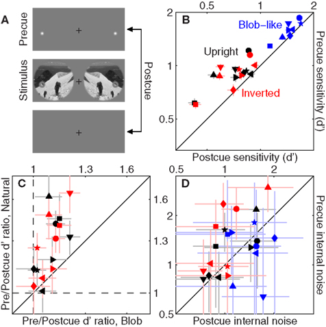
Figure 6. Effect of spatial cueing on sensitivity. We presented two spatial cues located at both target and non-target probes on each trial [top icon in (A)]; on some trials (randomly selected) the cues appeared before the stimulus (precue trials), on other trials they appeared after the stimulus (postcue trials). (B) Plots d′ for precue trials on the y axis versus d′ for postcue trials on the x axis. (D) Plots the same but for internal noise. (C) Plots ratios between d′ on precue trials and d′ on postcue trials, for blob-like images on the x axis versus natural (both upright in black and inverted in red) on the y axis. Dashed lines indicate unity ratios.
The first issue we address is whether the above-detailed manipulation was successful in inducing a differential use of attentional resources on the part of the human observers: although the precue offered the opportunity to achieve better performance, observers may have failed to exploit it effectively or even simply ignored it. Figure 6B unequivocally demonstrates that the manipulation was successful across the board: we observed a significant improvement in sensitivity on precue trials (y axis) as opposed to postcue trials (x axis) for all conditions (black points lie above the unity line at p < 0.005, red points at p < 0.01, blue points at p < 0.005). Clearly observers did exploit the cue effectively.
An interesting feature of the data plotted in Figure 6B is that there appeared to be greater benefit from using the cue for natural images (whether upright or inverted) as opposed to blob-like images: black/red points lie further away from the unity line than blue points (on a log–log plot). We quantify this effect in Figure 6C, where we assess the effect of the cue by plotting the ratio between sensitivity on precue trials and sensitivity on postcue trials. As expected the ratio values are all >1 (larger sensitivity on precue trials) shown by data points falling above the horizontal dashed line and to the right of the vertical dashed line (both lines indicate unity). This effect however is significantly larger for natural images, plotted on the y axis, as opposed to blob-like images, plotted on the x axis: data points fall above the solid unity line for both upright and inverted natural images (p < 0.02). This difference presumably results from the fact that the location of target/non-target probes was more readily identifiable against the relatively homogenous blob-like background as opposed to cluttered natural scenes, making the cue less valuable for the former class of images. We also assessed the impact of the cue on internal noise, plotted in Figure 6D for precue trials on the y axis versus postcue trials on the x axis. Perhaps surprisingly, we found a significant effect of the cue on internal noise for processing inverted natural images (red points lie above the unity line at p < 0.04) but not for the other two image classes (black symbols fall on unity line at p < 0.19, blue symbols at p < 0.4).
Figure 7 displays the characteristic structure for shape-index variation across image classes which we demonstrated previously (Figure 5C), plotted here separately for precue (Figure 7A) and postcue (Figure 7B) trials (we used smoothed filter estimates for this analysis due to the data reduction resulting from halving the dataset, Section 2.5). Clearly the same structure is present in both conditions. More specifically, oddity is greater than 0 for upright natural images (black symbols) on both precue (p < 0.03) and postcue (p < 0.04) trials, but is no different from 0 for inverted natural images in both conditions (p = 0.96 and p = 0.74 respectively).
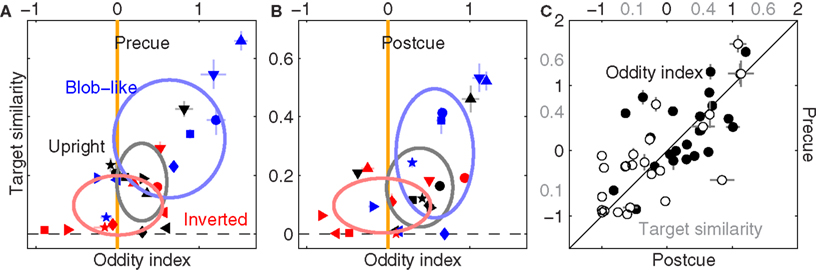
Figure 7. Effect of spatial cueing on filter shape. (A,B) Are plotted to the same conventions of Figure 5C, but report data for precue and postcue trials separately. (C) Plots all oddity (solid) and target similarity (open) estimates across conditions and observers for precue (y axis) versus postcue (x axis). Axis labels for target similarity in (C) are shown in gray.
To further emphasize the similarity between precue and postcue data, we plot each measurement from the precue dataset on the y axis versus each corresponding measurement from the postcue dataset on the x axis (pooling across image classes and observers without distinction), separately for the oddity index (solid) and the target-similarity index (open). We found a strong and significant positive correlation in both cases (r = 0.6 at p < 0.002 and r = 0.73 at p < 10−4 respectively). We conclude from this analysis that the context-dependent alterations in filter shape we reported in Figure 5 are unrelated to attentional deployment. This result is broadly consistent with previous experiments on the potential interaction (or lack thereof) of spatial cues with semantic manipulations of image content (Biederman, 1972).
3.4 Role of Phase Spectrum
Previous work in natural image processing has emphasized the distinction between power and image spectra (Morrone and Burr, 1988; Felsen et al., 2005; Bex et al., 2007). The generally held notion is that the phase spectrum, not the power spectrum, contains critical information for image interpretation (Piotrowski and Campbell, 1982). Recent work however has demonstrated that the power spectrum may contain more information than previously suspected (Torralba and Oliva, 2003), well beyond the 1/f2 trend that is known to characterize natural scenes (Ruderman and Bialek, 1994). We wished to relate our findings to this body of literature by manipulating our image dataset in similar ways. For each natural image in our database we created a “phase-only” image which preserved the phase spectrum of the original image but not its power spectrum, and a “power-only” image which preserved the power spectrum but not the phase spectrum (see Section 2.1). For the image in Figure 1A, the corresponding phase-only and power-only images are shown in Figures 8A and 11A respectively. We discuss results for the phase-only condition first.
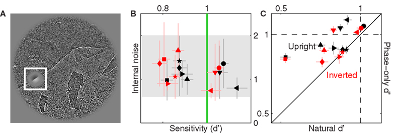
Figure 8. Sensitivity to phase-only images. (A) Shows Figure 3A following the phase-only manipulation (see Section 2.1). (B) Is plotted to the same conventions used in Figure 3D. (C) Plots d′ for the original natural images on the x axis, versus d′ for the phase-only dataset on the y axis.
Figure 8B shows sensitivity and internal noise values for phase-only images using the same plotting conventions adopted for the original images in Figure 3D. Internal noise lies within the same range (compare data position along the y axis between Figures 8B and 3D with respect to the gray shaded region). Sensitivity also lies within a similar range (near 1), but the phase-only data appears to fall at slightly higher values (black and red symbols in Figure 3D fall to the left of the green vertical line, whereas they scatter around this line in Figure 8B). We verify this effect in Figure 8C where we plot sensitivity for phase-only images on the y axis versus sensitivity for the original images on the x axis; phase-only sensitivity is larger for both upright and inverted images (black and red symbols fall above the unity line at p < 0.02 and p < 0.04 respectively). We speculate that this difference may have resulted from the fact that, similarly to blob-like images, the location of target/non-target probes was more readily identifiable against phase-only backgrounds, making the task easier. This speculation was confirmed by differential analysis of the data for precue and postcue trials, detailed below.
Figure 9A plots the sensitivity ratio between phase-only values and original image values, separately for precue trials on the y axis versus postcue trials on the x axis. On postcue trials, all ratios are >1 [data points fall to the right of the vertical dashed line at p < 0.02 for upright (black) condition and p < 0.03 for inverted (red) condition]. This effect is not significant for precue trials: ratios are >1 (data points fall on the horizontal dashed line at p > 0.05 for both upright and inverted). In other words, performance was higher for phase-only images compared to the original natural images when no spatial cues were provided ahead of the stimulus; when observers were cued, their performance was no different for the two image classes. It should be noted that previous studies have typically found that performance is degraded following removal of the power spectrum (Gaspar and Rousselet, 2009), opposite to what we found here. However the task adopted here is not comparable to those used in previous studies, a likely reason for this apparent discrepancy.
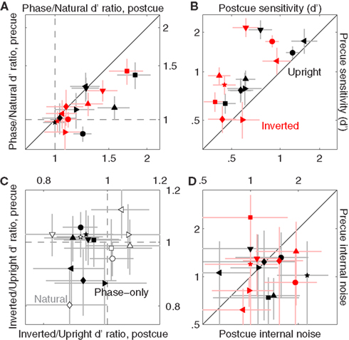
Figure 9. Comparison between sensitivity to natural and phase-only images. (A) Plots the ratio between d′ for phase-only images and d′ for natural (unmanipulated) images, from precue trials (y axis) versus postcue trials (x axis). Dashed lines indicate unity ratios. (B) Plots d′ for phase-only images, from precue trials (y axis) versus postcue trials (x axis); (D) plots internal noise in the same way. (C) Plots the ratio between d′ for inverted images and d′ for upright images, from precue trials (y axis) versus postcue trials (x axis) and for both the original images (open) and the phase-only images (solid).
We also noticed another, more interesting cue-specific effect: sensitivity was degraded by image inversion for phase-only images on postcue trials. This effect is to some extent visible in Figure 9B, where sensitivity on precue trials is plotted on the y axis versus sensitivity on postcue trials on the x axis, for the phase-only image dataset (this figure is the equivalent of Figure 6B for the original image dataset). Besides the clear cueing effect already demonstrated for the original images (points lie above the unity line at p < 0.02 for both upright and inverted), the inverted values appear to be shifted to the left of the upright values (compare each black symbol with each corresponding red symbol): an inversion effect for postcue, but not precue, trials. We document this effect more transparently in Figure 9C, where the inverted/upright sensitivity ratio is plotted for precue trials on the y axis versus postcue trials on the x axis. Ratios for phase-only images (solid) are ∼1 on precue trials (solid data points fall on horizontal dashed line at p = 0.28), but <1 on postcue trials (solid data points fall to the left of vertical dashed line at p < 0.001). This effect is absent for the original image database (open data points fall on the horizontal dashed line at p = 0.66 and on the vertical dashed line at p = 0.54) as expected from our previous analysis (see Figure 6).
As we did for the original image database, we also compared internal noise between precue and postcue trials for phase-only images. Internal noise values on precue trials are plotted on the y axis in Figure 9D, versus corresponding values for postcue trials on the x axis. We did not find any cue-specific effect (points fall on the unity line at p = 0.33 and p = 0.83 for upright and inverted respectively), differently from the original database (for which we measured a cue-specific effect in the inverted condition, see Figure 6D).
We analyzed phase-only perceptual filters using the same metrics described previously and confirmed the presence (although somewhat weaker) of an inversion effect on filter shape. Figure 10A is plotted to the same conventions as Figure 5C (and similarly relies on raw filter estimates; the blob-like data has been replicated here to ease direct comparison). It is clear that the same pattern is observed; more specifically, the upright condition is significantly odd (black symbols lie to the right of the orange line at p < 0.04) but this effect is not present for inverted images (red data points fall on the orange line at p = 0.21), despite both conditions being associated with SNR values significantly greater than baseline (at p < 0.05, not shown).
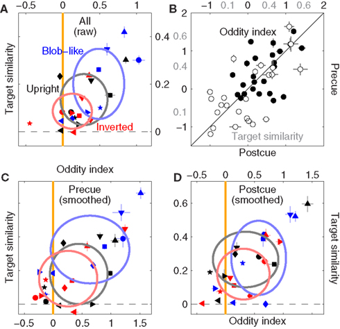
Figure 10. Filter shape metrics for phase-only images. (A) Is the equivalent of Figure 5C, (B) is the equivalent of Figure 7C, (C,D) are the equivalent of Figures 7A,B; all report data for the phase-only manipulation as opposed to the original unmanipulated images.
In line with the result reported earlier for natural images (Figure 7) precue and postcue conditions behaved similarly (Figure 10B) with relation to both oddity (correlation coefficient for solid symbols was 0.5 significant at p < 0.02) and target similarity (open symbols, r = 0.63 significant at p < 0.001). However the resolving power of our data diminished when we analyzed precue and postcue conditions separately in more detail: Figures 10C,D are the equivalent of Figures 7A,B (and similarly rely on smoothed filter estimates) but report data for phase-only images. On precue trials (Figure 10C) the oddity index generated the same pattern reported in 10A: upright but not inverted images show significant oddity (at p < 0.05 and p = 0.19 respectively); on postcue trials (Figure 10B) oddity for both conditions was not significantly different from 0 (at p > 0.05). The results from the cue-specific analysis are clearly less robust, but also more difficult to interpret because SNR was not significantly greater than 0 for either image type or cueing condition (at p > 0.05, not shown), and (as detailed previously) oddity can depend on SNR; it is also relevant in this context that we collected less trials for the phase-only condition (see Section 2.3), so it is possible that we were not able to resolve data structure as effectively due to insufficient data.
With the caveat detailed above relating to dataset size, we conclude that removing the information provided by the power spectrum somewhat reduces the effects we observed for context-dependent shape alterations in the structure of the perceptual filters. The effects are clearly still present (Figure 10A), but appear less robust when the dataset is halved for the purpose of probing specific subconditions (Figures 10C,D). It would appear that both phase and power information contribute to the alterations of filter shape we reported in Figure 5.
3.5 Role of Power Spectrum
We attempted to gather similar data for the power-only image dataset in order to study the effect of selectively removing phase information, but found that observers were unable to perform the task when this image manipulation was applied; spatial cueing did not help. Figure 11C plots sensitivity on precue trials (y axis) versus sensitivity on postcue trials (x axis) for the power-only image dataset when noise intensity was set to zero and target intensity to the largest value afforded by the operating range of our monitors. Under these conditions the target edge is perfectly visible, and observers scored perfect performance (100% correct responses) for the original image database. Following removal of phase information, performance plummets to near chance and the corresponding sensitivity values never exceed 1 on either precue or postcue trials (with no difference between them: data points fall on the unity line in Figure 11C at p = 0.79).
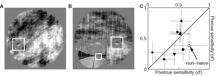
Figure 11. Sensitivity to power-only images. (A) Shows Figure 3A following the power-only manipulation (see Section 2.1). (B) Shows another example: the original image is displayed in the inset, the power-only version in the main panel. (C) Plots d′ from precue trials (y axis) versus postcue trials (x axis); no distinction was made between upright and inverted conditions because not relevant. Open symbol shows data for author Peter Neri.
We confirmed this result in a non-naive observer (author Peter Neri) who had full knowledge of how the stimuli were generated; data for this observer is indicated by the open symbol in Figure 11C and is within the range spanned by the naive observers. This state of affairs made it impossible to proceed with further data collection because our methodology relies on threshold levels of target intensity (Ahumada, 2002; Neri and Levi, 2006): consider that observers were performing well below the desired sensitivity level of d′ ∼ 1 in the absence of any noise and in the presence of a highly visible signal. Adding noise would reduce performance even further, making it impossible to select target intensity values that would afford viable reverse correlation experiments (Murray et al., 2002). Clearly performance in these conditions is primarily limited by factors that are not under the control of the external noise source, forcing us to abandon this line of investigation.
The extremely poor performance we observed for power-only images is easily explained when one considers the nature of the task in conjunction with the effect of removing phase information from specific image samples. Figure 11A shows the power-only version of the image in Figure 1A. For this particular image the orientation of the target edge happens to match the overall orientation content of the picture; even if phase information is removed, the residual power information allows for a match between target edge and surrounding context (Figure 11A) and the task can be performed. But consider Figure 11B: the original scene (lower-left inset) presents a clear match between target orientation and the local orientation of the image (defined by the edge of the road); across the whole image, however, most power lies in the vertical orientation (main panel in Figure 11B) which is not the orientation of the target. For this specific natural scene observers would find it impossible to decide whether the target should be oriented as shown in Figure 11B, or orthogonal to it. Because this situation is relatively common across our database, the resulting performance level is prohibitively poor.
3.6 Role of Image Content (Scenes Versus Faces)
Our database spanned a wide range of image material: cities, built outdoors, forests, mountains, faces (see Figure A2 in Appendix for a selection of representative examples). We investigated the possibility that some of the effects we reported earlier showed specificity for image content. In keeping with previous literature (Wright and Roberts, 1996; Yovel and Kanwisher, 2005; Epstein et al., 2006) we focused our analysis on the distinction between scenes (Figure 12A) and faces (Figure 12B). We observed clear differences in sensitivity (but not internal noise): probes were processed more efficiently when embedded within scenes as opposed to faces (all points lie above the unity line in Figure 12C at p < 0.05), no matter whether they were upright or inverted (black and red symbols) and precued or postcued (solid and open symbols). Interestingly this effect was partly dependent upon the power spectrum because it was less pronounced for phase-only images: the ratio between sensitivity for scenes and sensitivity for faces (plotted in Figure 12D) was larger for natural images (x axis) as opposed to phase-only images (data points fall below the unity line at p < 0.02 for upright and p < 0.01 for inverted). Notice however that the effect, although smaller, was nevertheless present after removal of the power spectrum (points fall above the horizontal dashed line at p < 0.02 for both upright and inverted), demonstrating a role for the phase spectrum.
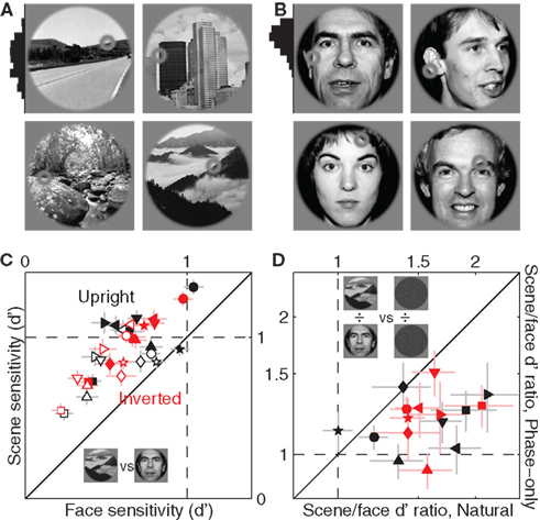
Figure 12. Sensitivity to scenes versus faces. (A) Shows four scenes from the database, (B) shows four faces. Histogram to the right of image in (A) shows distribution of probe locations (across the entire scene database) along the vertical extension of the image; histogram in B shows the same for faces. (C) Plots d′ for scenes (y axis) versus d′ for faces (x axis), from both precue (solid) and postcue (open) trials. (D) Plots ratio between d′ for scenes and d′ for faces, for natural images on the x axis versus phase-only images on the y axis.
Turning images upside-down had little effect on sensitivity with no specificity for either faces or scenes. Previous reports (Wright and Roberts, 1996; Epstein et al., 2006) have highlighted a distinction between faces and scenes in this respect, whereby inversion effects apply primarily if not exclusively to faces. We therefore looked for this class of effects when restricted to our face dataset but could not find any (x values of black and red symbols in Figure 12C span similar ranges), not even in relation to the effect reported earlier that sensitivity was lower for inverted phase-only images (Figure 9C): this effect, very significant when data was pooled from both faces and scenes, was lost (at p > 0.05) when the dataset was restricted to either image category. We attribute this apparent discrepancy to the different nature of our task in comparison to those used by previous studies on the inversion effect (e.g., Yin, 1969; Wright and Roberts, 1996; Yovel and Kanwisher, 2005): in these previous tasks observers were not asked to discriminate local properties of the image, whereas this was a critical feature of our experimental design.
We also identified some specificity in relation to the context-dependence of filter shape. Figures 13A,B are the equivalent of Figure 5C plotted separately for faces (A) and scenes (B). Scenes mostly conform to the pattern we have discussed previously: upright natural scenes and blob-like images are significantly odd (black symbols fall to the right of the vertical orange line at p < 0.0002, blue symbols at p < 0.02), while inverted images are not (red symbols fall on vertical orange line at p = 0.1); furthermore, upright natural scenes show larger target similarity than inverted scenes (black symbols are shifted upwards of red symbols at p < 0.02). There is also a trend for upright natural scenes to show larger oddity and target similarity than blob-like images (black cluster is located above and to the right of blue cluster). Data for faces (A) differs in that upright natural faces are not significantly odd (black symbols scatter around vertical orange line at p = 0.62), and there is no difference in target similarity between upright and inverted (p = 0.3). The similarity in perceptual filters for upright and inverted faces is consistent with previous reports using psychophysical reverse correlation (Sekuler et al., 2004). The different outcome for upright faces versus scenes is shown more clearly in Figure 13C, where oddity is plotted for scenes (y axis) versus faces (x axes); all black points lie above the solid unity line (direct comparison) at p < 0.02, indicating larger oddity for upright scenes as opposed to upright faces.
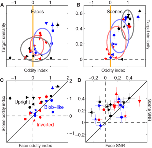
Figure 13. Differential effect of scenes versus faces on filter shape. (A,B) Are plotted to the same conventions of Figure 5C, separately for faces (A) and scenes (B). (C) Plots oddity index for scenes (y axis) versus faces (x axis); (D) reports filter SNR using similar plotting conventions. Data has been pooled from both natural and phase-only datasets.
The above-detailed effects on filter shape are tentative for three reasons. First, filter SNR values were occasionally not different from 0 (Figure 13D); as mentioned previously SNR values close to 0 pose a serious problem for interpreting the oddity index correctly. More specifically, upright perceptual filters returned SNR values greater than 0 only for scenes (p < 0.0002), not faces (p = 0.27); SNR values for inverted filters were greater than 0 for both scenes and faces (p < 0.05). Second, because the probability of selecting a face was 1/2 the probability of selecting a scene on a given trial (see Section 2), twice more data was collected for scenes than for faces; it is therefore possible that the lack of an oddity effect for upright images may have resulted from insufficient data [however we were able to resolve the effect for blob-like images from faces (blue symbols) with far less data (by a factor of ∼2 because no phase-only trials were collected for blob-like images), which would seem to argue against this interpretation]. Third, the face dataset and the natural scene dataset differed in obvious ways that may have little relevance to the semantic distinction between faces and scenes: face images were more homogeneous in structure than scene images (see Figure A2 in Appendix), while this is not necessarily true in natural vision. Furthermore the outcome of our automated probe-insertion algorithm was such that face images, but not scenes, showed a biased distribution of probe locations: probes were mostly located within the eye region in face images (see histogram to the left of Figure 12B), whereas there was no upper-lower bias for scenes (histogram to the left of Figure 12A). While this factor highlights potential low-level differences between face and scene datasets, it indicates that the scene images were relatively uniform in their edge structure across the vertical dimension, further strengthening the notion that image inversion was specifically targeting higher-level and not lower-level aspects of the scenes.
3.7 Modeling
The main purpose of the modeling exercise was to identify the minimal elements required for a qualitative account of the most prominent features of the perceptual filters; it was not intended as a comprehensive model of all the effects reported in this study. A model of the latter kind would need to account for the effect of image inversion; because this effect is exclusively higher-level (Valentine, 1988) the model would need to interpret the semantic content of the image. Although there exist models that incorporate semantic knowledge (e.g., Ullman et al., 2002), none has been described in sufficient detail to afford implementation within the context of our experiments; the development of such models for application to our data is well beyond the scope of the present study. A secondary goal of the simulations we present in Figure 14 (discussed below) was to provide indirect validation for the combination rule we adopted in order to compute the perceptual filter (see Figure 2 and Section 2.5).
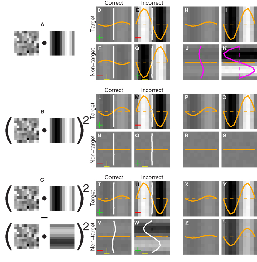
Figure 14. Simulated perceptual filters. We tested three simple models, starting with linear template matching (A). The model in (B) is the same as (A), except the output of the matching operation is squared. (C) Is the same as (B) minus the output of a unit orthogonal to (B) with reduced gain. See Section 2.8 for details. The average noise images associated with the classification carried out by the different models are shown in (D–K) for model (A), (L–S) for model (B), and (T–Σ) for model (C). Each set is plotted to the conventions of Figures 2A–H.
In the absence of modeling, it may be expected that a simple template-matching strategy should return the observed perceptual filters. Figure 14A outlines a model of this kind: the input image is matched to an oriented grating via inner product (•), and the resulting output is used to generate a psychophysical choice (see Section 2.8). As shown in Figures 14D–K this approach generates filters that are inconsistent with those observed experimentally: the perceptual filter computed from non-target noise fields on incorrect trials (Figure 14G) is oriented orthogonally to that measured in the human observers (see magenta trace and compare Figure 14K with Figure 2H); a similar result was obtained for non-target noise fields on correct trials (Figure 14J). We must therefore abandon the template-matching model (also known as linear–non-linear cascade), despite its common application in sensory neuroscience (Marmarelis, 2004; Sharpee et al., 2008) and its significance in relation to reverse correlation methods (Ahumada, 2002; Murray et al., 2005; Neri, 2010b).
A simple, plausible modification of the model in Figure 14A leads to improved simulation of the human data: the output from the template-matching stage is squared as indicated in Figure 14B. The resulting perceptual filters are now closer to those observed experimentally: no filter in Figures 14L–S presents structure orthogonal to the human data, and the filter derived from target-present noise fields on incorrect trials (Figure 14M) has larger amplitude than the other subfilters as in the human data (compare with Figure 2). There are nevertheless some residual differences, in particular the lack of modulation for some of the subfilters (Figures 14R–S). This issue can be rectified by subtracting the output from an orthogonally oriented unit in a push–pull fashion as outlined in Figure 14C (see Section 2.8). The resulting subfilters, shown in Figure 14X–Σ, capture most of the features seen in the human data (compare with Figures 2E–H). We also verified that shape manipulations of the model filters affected the three metrics we used (oddity, target similarity and fitted phase) in a sensible, predictable manner: when we varied the phase of the gratings we found (as expected) that this parameter was highly correlated with all three shape indices; for example, the oddity index decreased as we manipulated the phase of the gratings to approach a cosine (rather than sine) profile.
An interesting prediction associated with the model in Figure 14C is that observers should be insensitive to the polarity of the target edge. In other words, if observers were asked to discriminate between the target edge and a non-target edge of the same orientation but with swapped bright and dark regions, their performance should be at chance. This is indeed the case, as we verified during the preliminary stages of design and protocol development: perhaps surprisingly, it is virtually impossible to discriminate edge polarity for the peripheral presentation employed in this study, even in the absence of any noise within the probe. This observation also serves as a useful reminder of the potential limitations associated with the specific protocol used here: our results pertain to peripheral processing. While it is attractive to speculate that they may extend to the fovea, known differences between these two structures prompt caution. Crowding in particular, a well-known phenomenon that likely played a role in our experiments, is primarily if not exclusively operational in the periphery (Levi and Carney, 2009; it is worth noting however that crowding is expected to be equally effective for upright and inverted stimuli, making it unlikely that it would provide an explanation for the differences we report between these two conditions). A related potential limitation of our experiments is that we only tested one probe size; the choice of this specific size (roughly 1°) was motivated by the similar size of V1 receptive fields at the eccentricities tested (Dumoulin and Wandell, 2008). We do not know whether/how the results reported here may extend to smaller/larger probes.
4 Discussion
4.1 Context-Dependent Effects on Sensitivity and Filter Shape
We measured effects of image statistics on both sensitivity and filter shape. The effects on sensitivity were robust (e.g., Figures 3E and 9A) and partly interpretable based on simple considerations about image structure following the different manipulations we applied (e.g., the relative ease of locating probes against blob-like and phase-only backgrounds, Section 3). We occasionally measured robust effects for which there was no obvious explanation: the advantage for processing scenes over faces was greatly reduced (although not eliminated) by removal of the power spectrum (Figure 12D).
To assess the robustness of our filter measurements we rely on replicability across the dataset. The main result from our analysis of context-dependent effects on the estimated perceptual filters is indicated by the pattern in Figure 5C; this pattern was independently demonstrated on three separate instances: for precue (Figure 7A), postcue (Figure 7B) and phase-only manipulations (Figure 10A) from three entirely distinct datasets. It is clear that we extracted genuine data structure in relation to the effect of image statistics on filter shape, despite the challenging task of achieving this goal via an indirect probe-image coupling design (Figure 1), sizeable internal noise (Figure 3D), the necessity to obtain a large amount of data (we collected in excess of 180 K trials for this study) and the intrinsically noisy nature of the reverse correlation methodology.
We can sketch an intuitive interpretation for the effects we measured on filter shape. Both oddity and target similarity reflect how well the perceptual filter is matched to the target edge (although the oddity index has more general value, Section 3.2). If we adopt this simple interpretation, then the main pattern we observed for context-dependent changes in filter shape (Figure 5C) indicates that filter affinity for target shape is degraded by image inversion. We propose the following conceptual model for a qualitative interpretation of this result. In line with current thinking about simple feature detection, each location in the visual field is analyzed by both edge (odd) and line (even) detectors (Pollen and Ronner, 1981; Morrone and Burr, 1988). For the purpose of performing the edge-detection task we assigned to our observers, image context is exploited by the visual system to bias the output of detectors within the localized probe region in favor of the odd subpopulation so as to extract primarily odd (edge-like) energy. We hypothesize that the process of biasing the local detection machinery is affected by a higher-level interpretation of the image; when this interpretation is disrupted by inverting the image upside-down, the biasing signal is weaker and local detection retains roughly equal odd/even components.
The interpretation above is very speculative and by no means exclusive of others, so we only offer it as a coarse tool for a potentially intuitive understanding of our results. Our main conclusion is independent of this specific model. We also emphasize that this interpretation does not imply that the changes we report for the behavioral perceptual filter directly reflect changes at the level of the earliest edge-detection devices in the human brain, e.g., edge-selective neurons in primary visual cortex. Our measurements are behavioral; as such, they monitor the output of a relatively large neuronal circuit. This means that the perceptual filters reported here return an aggregate picture of several neuronal receptive fields. Any associated change in oddity may result from a change in the relative output of some circuit elements compared to others (e.g., odd as opposed to even), without any qualitative change in the response selectivity of the individual elements. This is the interpretation we favor. In this context we use the term “human edge detector” to refer to the entire circuit; we would contend that, despite its being more complex than a single element, this aggregate entity falls within the domain of low-level vision insofar as this terminology is currently understood and conceptualized in the field.
4.2 Low-Level Manipulations Affect Sensitivity, Higher-Level Manipulations Affect Filter Shape
To facilitate a coherent interpretation of our results we draw a distinction between two broad categories of experimental manipulations: low-level and higher-level. By low-level manipulations we refer to all image comparisons except for upright versus inverted (see Section 2.7 for details). Together with manipulations that introduce obvious differences in image statistics [i.e., visible via coarse inspection of the Fourier transform (Torralba and Oliva, 2003)] we include the distinction between faces and scenes because these two image classes differ in several low-level respects, as well as the attentional manipulation because cueing alters the local spatiotemporal properties of the stimulus.
By higher-level comparisons we refer to those that are not explained by image statistics per se, i.e., effects based on a comparison between upright and inverted images. Although image inversion clearly affects the Fourier transform, the associated changes are invisible to early visual cortex (Kayser et al., 2004). If we consider the power spectrum for different image orientations, vertical and horizontal are not affected by inversion; diagonal orientations are, but because we presented images in a left–right mirror fashion (see Figures 1A,B) any such effect is irrelevant. A classifier that is able to recognize image inversion would need to incorporate more complex algorithms than those operating in the early stages of visual processing (Kayser et al., 2003; Yu et al., 2005; Geisler, 2008). For this reason any effect deriving from image inversion is believed to reflect higher-level processing (Valentine, 1988; Wright and Roberts, 1996; Yovel and Kanwisher, 2005); we adopt the same view here.
Taken together and with a few notable exceptions (e.g., Figures 9C and 6D) our dataset points to the following result: low-level image manipulations result primarily in sensitivity changes, with little evidence of changes in filter shape; conversely, higher-level manipulations result primarily in modified filter shape with little evidence of changes in sensitivity. Figure 15 summarizes our entire dataset within the context of this conceptual framework. Low-level image manipulations (black symbols) lead to sizeable sensitivity changes (x axis) but have a small effect on filter shape (y axis), as demonstrated by the relevant data points stretching along the x axis (black points fall to the right of the vertical dashed line at p < 10−18). Higher-level manipulations (red symbols) generate a complementary pattern, as demonstrated by the relevant data points stretching along the y axis (red points fall above the horizontal dashed line at p < 0.002). More specifically, the average change in performance metric index (x axis) is 6.5 times larger for low-level manipulations as opposed to higher-level manipulations; this effect is significant at p < 10−6 (unpaired two-tailed t-test). Conversely, the average change in filter shape index (y axis) is 4.6 times larger for higher-level manipulations as opposed to low-level manipulations and this effect is significant at p < 0.001.
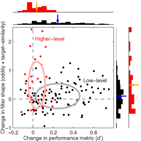
Figure 15. Low-level manipulations change sensitivity, higher-level manipulations change filter shape. Change in sensitivity (d′ log-ratio) is plotted on the x axis versus change in filter shape (y axis) as assessed using an index that combines both oddity and target similarity (see Section 2.7), for both low-level image manipulations (e.g., blob-like transformation) in black and higher-level manipulations (image inversion) in red. See Section 2.7 for details on how different comparisons were classified as low-level or higher-level. Top and right histograms plot distributions; arrows show mean values.
4.3 Sensitivity and Filter Shape: Different Tools for Different Jobs
Is it reasonable to expect a dissociation between sensitivity metrics and filter characteristics of the kind reported in Figure 15? If we accept the notion that observers rely on perceptual filter machinery to perform the task, then it may appear that sensitivity and filter shape should be coupled in a simple way. However this expectation critically depends on the assumption that the system operates like a linear amplifier (Ahumada, 2002; Neri, 2010b); for this specific class of models sensitivity can be predicted from filter shape (Murray et al., 2005). When the system is not well-captured by linear models, the relationship between filter shape and sensitivity becomes opaque (Murray et al., 2005). There are now several demonstrations in the literature that filter shape and sensitivity can be decoupled and provide differential insight into the process of interest; we briefly consider three examples from independent laboratories. In previous work (Neri and Levi, 2007) we reported that filter dynamics is affected by figure-ground segregation without any associated change in sensitivity; a simple model was able to account for both results. A subsequent study (Nagai et al., 2008) was able to measure a vertical bias for contour completion from filter shape but not from sensitivity thresholds, and a very recent study (Dobres and Seitz, 2010) relied on filter shape to reveal aspects of perceptual learning that could not be exposed with standard performance metrics.
It is also clear from previous research that the linear amplifier model is often inapplicable due to the presence of significant non-linearities (Abbey and Eckstein, 2006; Neri, 2010b; see also Machens et al., 2004). Our simulations indicate that a linear model is inadequate for a correct interpretation of the data we report here (see Figure 14 and its relevance to Figure 2). Insertion of a non-linear processing layer into any proposed model for simulating human performance makes it unsurprising that filter shape and sensitivity may be manipulated independently and behave in a largely decoupled fashion as empirical quantities (Abbey and Eckstein, 2006; Neri, 2010b). The dissociation we demonstrate in Figure 15 is therefore compatible with existing literature (see previous paragraph) and theoretical notions. It likely reflects a simple fact: different metrics from different methodologies provide different kinds of information about the process of interest (Neri and Levi, 2007; Nagai et al., 2008; Dobres and Seitz, 2010), each metric with its own resolving power in relation to specific experimental manipulations.
5 Conclusion
Our primary result is grounded on data, regardless of specific models and/or conceptual frameworks. It consists of the largely unexpected result that higher-level manipulations of image content (i.e., inverting the image upside-down) altered the characteristics of local edge detectors employed by the human observers for feature extraction (see Figure 15). No existing model can account for this effect. Our results demonstrate that even the earliest and simplest stages in human visual processing cannot be fully understood as operating completely outside the domain of higher-level processing; a comprehensive account of low-level vision requires that feature detectors are characterized not only within the controlled parameter range spanned by artificial stimuli (Rust and Movshon, 2005), but also within the operating regime afforded by natural statistics (Felsen and Dan, 2005).
Conflict of Interest Statement
The author declares that the research was conducted in the absence of any commercial or financial relationships that could be construed as a potential conflict of interest.
Acknowledgments
Supported by Royal Society and Medical Research Council.
References
Abbey, C. K., and Eckstein, M. P. (2006). Classification images for detection, contrast discrimination, and identification tasks with a common ideal observer. J. Vis. 6, 335–355.
Ahumada, A. J. (2002). Classification image weights and internal noise level estimation. J. Vis. 2, 121–131.
Bennett, P. J., and Banks, M. S. (1991). The effects of contrast, spatial scale, and orientation on foveal and peripheral phase discrimination. Vision Res. 31, 1759–1786.
Bex, P. J., Mareschal, I., and Dakin, S. C. (2007). Contrast gain control in natural scenes. J. Vis. 7, 1–12.
Bex, P. J., Solomon, S. G., and Dakin, S. C. (2009). Contrast sensitivity in natural scenes depends on edge as well as spatial frequency structure. J. Vis. 9, 1–19.
Burgess, A. E., and Colborne, B. (1988).Visual signal detection. IV. Observer inconsistency. J. Opt. Soc. Am. A 5, 617–627.
Burr, D. C., Morrone, M. C., and Spinelli, D. (1989). Evidence for edge and bar detectors in human vision. Vision Res. 29, 419–431.
David, S. V., Vinje, W. E., and Gallant, J. L. (2004). Natural stimulus statistics alter the receptive field structure of v1 neurons. J. Neurosci. 24, 6991–7006.
Dobres, J., and Seitz, A. R. (2010). Perceptual learning of oriented gratings as revealed by classification images. J. Vis. 10, 1–11.
Dumoulin, S. O., and Wandell, B. A. (2008). Population receptive field estimates in human visual cortex. Neuroimage 39, 647–660.
Epstein, R. A., Higgins, J. S., Parker, W., Aguirre, G. K., and Cooperman, S. (2006). Cortical correlates of face and scene inversion: a comparison. Neuropsychologia 44, 1145–1158.
Felsen, G., Touryan, Han, F., and Dan, Y. (2005). Cortical sensitivity to visual features in natural scenes. PLoS Biol. 3, e342. doi: 10.1371/journal.pbio.0030342
Foulsham, T., and Underwood, G. (2008). What can saliency models predict about eye movements? Spatial and sequential aspects of fixations during encoding and recognition. J. Vis. 8, 1–17.
Frazor, R. A., and Geisler, W. S. (2006). Local luminance and contrast in natural images. Vision Res. 46, 1585–1598.
Gaspar, C. M., Bennett, P. J., and Sekuler, A. B. (2008). The effects of face inversion and contrast-reversal on efficiency and internal noise. Vision Res. 48, 1084–1095.
Gaspar, C. M., and Rousselet, G. A. (2009). How do amplitude spectra influence rapid animal detection? Vision Res. 49, 3001–3012.
Geisler, W. S. (2008). Visual perception and the statistical properties of natural scenes. Annu. Rev. Psychol. 59, 167–192.
Geisler, W. S., Perry, J. S., Super, B. J., and Gallogly, D. P. (2001). Edge co-occurrence in natural images predicts contour grouping performance. Vision Res. 41, 711–724.
Guo, K., Robertson, R. G., Mahmoodi, S., and Young, M. P. (2005). Centre-surround interactions in response to natural scene stimulation in the primary visual cortex. Eur. J. Neurosci. 21, 536–548.
Kayser, C., Kording, K. P., and Konig, P. (2004). Processing of complex stimuli and natural scenes in the visual cortex. Curr. Opin. Neurobiol. 14, 468–473.
Kayser, C., Salazar, R. F., and Konig, P. (2003). Responses to natural scenes in cat V1. J. Neurophysiol. 90, 1910–1920.
Levi, D. M., and Carney, T. (2009). Crowding in peripheral vision: why bigger is better. Curr. Biol. 19, 1988–1993.
Li, F. F., VanRullen, R., Koch, C., and Perona, P. (2002). Rapid natural scene categorization in the near absence of attention. Proc. Natl. Acad. Sci. U.S.A. 99, 9596–9601.
MacEvoy, S. P., Hanks, T. D., and Paradiso, M. A. (2008). Macaque V1 activity during natural vision: effects of natural scenes and saccades. J. Neurophysiol. 99, 460–472.
Machens, C. K., Wehr, M. S., and Zador, A. M. (2004). Linearity of cortical receptive fields measured with natural sounds. J. Neurosci. 24, 1089–1100.
Mante, V., Frazor, R. A., Bonin, V., Geisler, W. S., and Carandini, M. (2005). Independence of luminance and contrast in natural scenes and in the early visual system. Nat. Neurosci. 8, 1690–1697.
Marmarelis, V. Z. (2004). Nonlinear Dynamic Modeling of Physiological Systems. Piscataway, NJ: Wiley IEEE Press.
Meese, T. S., Hess, R. F., and Williams, C. B. (2005). Size matters, but not for everyone: individual differences for contrast discrimination. J. Vis. 5, 928–947.
Morrone, M. C., and Burr, D. C. (1988). Feature detection in human vision: a phase-dependent energy model. Proc. R. Soc. Lond. B Biol. Sci. 235, 221–245.
Murray, R. F., Bennett, P. J., and Sekuler, A. B. (2002). Optimal methods for calculating classification images: weighted sums. J. Vis. 2, 79–104.
Murray, R. F., Bennett, P. J., and Sekuler, A. B. (2005). Classification images predict absolute efficiency. J. Vis. 5, 139–149.
Nagai, M., Bennett, P. J., and Sekuler, A. B. (2008). Exploration of vertical bias in perceptual completion of illusory contours: threshold measures and response classification. J. Vis. 8, 1–17.
Neri, P. (2010a). How inherently noisy is human sensory processing? Psychon. Bull. Rev. 17, 802–808.
Neri, P. (2010b). Stochastic characterization of small-scale algorithms for human sensory processing. Chaos 20, 045118.
Neri, P., and Levi, D. M. (2006). Receptive versus perceptive fields from the reverse-correlation viewpoint. Vision Res. 46, 2465–2474.
Neri, P., and Levi, D. M. (2007). Temporal dynamics of figure-ground segregation in human vision. J. Neurophysiol. 97, 951–957.
Neri, P., and Levi, D. M. (2008). Evidence for joint encoding of motion and disparity in human visual perception. J. Neurophysiol. 100, 3117–3133.
Oliva, A., and Torralba, A. (2001). Modeling the shape of the scene: a holistic representation of the spatial envelope. Int. J. Comput. Vis. 42, 145–175.
Paradiso, M. A., Blau, S., Huang, X. S. P., MacEvoy, Rossi, A. F., and Shalev, G. (2006). Lightness, filling-in, and the fundamental role of context in visual perception. Prog. Brain Res. 155, 109–123.
Piotrowski, L. N., and Campbell, F. W. (1982). A demonstration of the visual importance and flexibility of spatial-frequency amplitude and phase. Perception 11, 337–346.
Pollen, D. A., and Ronner, S. F. (1981). Phase relationships between adjacent simple cells in the visual cortex. Science 212, 1409–1411.
Rieke, F., Bodnar, D. A., and Bialek, W. (1995). Naturalistic stimuli increase the rate and efficiency of information transmission by primary auditory afferents. Proc. Biol. Sci. 262, 259–265.
Ringach, D. L., Hawken, M. J., and Shapley, R. (2002). Receptive field structure of neurons in monkey primary visual cortex revealed by stimulation with natural image sequences. J. Vis. 2, 12–24.
Rousselet, G. A., Fabre-Thorpe, M., and Thorpe, S. J. (2002). Parallel processing in high-level categorization of natural images. Nat. Neurosci. 5, 629–630.
Ruderman, D. L., and Bialek, W. (1994). Statistics of natural images: scaling in the woods. Phys. Rev. Lett. 73, 814–817.
Sekuler, A. B., Gaspar, C. M., Gold, J. M., and Bennett, P. J. (2004). Inversion leads to quantitative, not qualitative, changes in face processing. Curr. Biol. 14, 391–396.
Sharpee, T. O., Miller, K. D., and Stryker, M. P. (2008). On the importance of static nonlinearity in estimating spatiotemporal neural filters with natural stimuli. J. Neurophysiol. 99, 2496–2509.
Simons, D. J., and Rensink, R. A. (2005). Change blindness: past, present, and future. Trends Cogn. Sci. (Regul. Ed.) 9, 16–20.
Smyth, D., Willmore, B., Baker, G. E., Thompson, I. D., and Tolhurst, D. J. (2003). The receptive-field organization of simple cells in primary visual cortex of ferrets under natural scene stimulation. J. Neurosci. 23, 4746–4759.
Tolhurst, D. J., Smyth, D., and Thompson, I. D. (2009). The sparseness of neuronal responses in ferret primary visual cortex. J. Neurosci. 29, 2355–2370.
Touryan, J., Felsen, G., and Dan, Y. (2005). Spatial structure of complex cell receptive fields measured with natural images. Neuron 45, 781–791.
Ullman, S., Vidal-Naquet, M., and Sali, E. (2002). Visual features of intermediate complexity and their use in classification. Nat. Neurosci. 5, 682–687.
Valentine, T. (1988). Upside-down faces: a review of the effect of inversion upon face recognition. Br. J. Psychol. 79(Pt 4), 471–491.
Vinje, W. E., and Gallant, J. L. (2002). Natural stimulation of the nonclassical receptive field increases information transmission efficiency in V1. J. Neurosci. 22, 2904–2915.
Woolley, S. M., Fremouw, T. E., Hsu, A., and Theunissen, F. E. (2005). Tuning for spectro-temporal modulations as a mechanism for auditory discrimination of natural sounds. Nat. Neurosci. 8, 1371–1379.
Wright, A. A., and Roberts, W. A. (1996). Monkey and human face perception: inversion effects for human faces but not for monkey faces or scenes. J. Cogn. Neurosci. 8, 278–290.
Yovel, G., and Kanwisher, N. (2005). The neural basis of the behavioral face-inversion effect. Curr. Biol. 15, 2256–2262.
Yu, C., and Levi, D. M. (2000). Surround modulation in human vision unmasked by masking experiments. Nat. Neurosci. 3, 724–728.
Keywords: visual psychophysics, reverse correlation, inversion effect, top-down
Citation: Neri P (2011) Global properties of natural scenes shape local properties of human edge detectors. Front. Psychology 2:172. doi: 10.3389/fpsyg.2011.00172
Received: 29 April 2011; Accepted: 11 July 2011;
Published online: 05 August 2011.
Edited by:
Peter J. Bex, Massachusetts Eye and Ear Infirmary, USAReviewed by:
Carl M. Gaspar, University of Glasgow, UKCraig Abbey, University of California Santa Barbara, USA
Copyright: © 2011 Neri. This is an open-access article subject to a non-exclusive license between the authors and Frontiers Media SA, which permits use, distribution and reproduction in other forums, provided the original authors and source are credited and other Frontiers conditions are complied with.
*Correspondence: Peter Neri, Institute of Medical Sciences, Aberdeen Medical School, Foresterhill AB25 2ZD Aberdeen, UK. e-mail: peter.neri@abdn.ac.uk