Response Errors Explain the Failure of Independent-Channels Models of Perception of Temporal Order

Independent-channels models of perception of temporal order (also referred to as threshold models or perceptual latency models) have been ruled out because two formal properties of these models (monotonicity and parallelism) are not borne out by data from ternary tasks in which observers must judge whether stimulus A was presented before, after, or simultaneously with stimulus B. These models generally assume that observed responses are authentic indicators of unobservable judgments, but blinks, lapses of attention, or errors in pressing the response keys (maybe, but not only, motivated by time pressure when reaction times are being recorded) may make observers misreport their judgments or simply guess a response. We present an extension of independent-channels models that considers response errors and we show that the model produces psychometric functions that do not satisfy monotonicity and parallelism. The model is illustrated by fitting it to data from a published study in which the ternary task was used. The fitted functions describe very accurately the absence of monotonicity and parallelism shown by the data. These characteristics of empirical data are thus consistent with independent-channels models when response errors are taken into consideration. The implications of these results for the analysis and interpretation of temporal order judgment data are discussed.

Introduction

Judgments of the temporal order or simultaneity of two stimuli are collected in studies of prior entry, multisensory integration, or causality perception (Schneider and Bavelier, 2003; Stetson et al., 2006; Spence and Parise, 2010; Vroomen and Keetels, 2010; Yates and Nicholls, 2011) and, more generally, in research on perception of temporal order (Sternberg and Knoll, 1973; Occelli et al., 2011). The two stimuli that are involved may pertain to different sensory modalities but, without loss of generality, we will assume the audiovisual case in the following description. In these experiments, visual and auditory stimuli are presented with a range of auditory delays (or stimulus onset asynchrony, SOA), defined as the difference between the onset of the auditory stimulus and that of the visual stimulus. In the ternary version of the simultaneity judgment task (SJ3 task; Ulrich, 1987), the observer must judge whether the auditory stimulus was presented before, after, or simultaneously with the visual stimulus, yielding “audio-first” (AF), “video-first” (VF), or “simultaneous” (S) responses.

Models of timing judgments fall within the class of independent-channels models described by Sternberg and Knoll (1973), in which signals from the two stimuli reach a central mechanism with randomly distributed arrival latencies. At the central mechanism, the judgment arises on application of a decision rule to the arrival-time difference between the signals. Sternberg and Knoll derived general properties of independent-channels models without making assumptions about the distribution of arrival latencies or about the form of the decision rule. With explicit assumptions about these components, independent-channels models yield expressions for the psychometric functions Ψ_AF, Ψ_S, and Ψ_VF, respectively describing how the probabilities of AF, S, and VF judgments vary with auditory delay. Sternberg and Knoll also showed that the attention-switching models of Kristofferson and Allan (1973) can be cast in terms of independent-channels models and, thus, they do not represent an essentially different type of models as regards the issues addressed in this paper.

A theoretically important feature of independent-channels models of perception of temporal order is that they entail a representation of the processes governing observed performance at timing judgment tasks. Model parameters are thus straightforwardly interpretable as reflecting characteristics of the distributions of arrival latencies (determined by sensory transmission and perceptual processing), and they also characterize the observer as a decision maker whose judgments rely on sensory information, subject to limitations imposed by the temporal resolution with which observers can tell small differences in arrival latency. These models are thus useful in studies of prior entry or temporal recalibration because parameter estimates directly indicate how experimental manipulations affect either the distributions of arrival latencies or the operating temporal resolution of the observer.

However, empirical tests of the models revealed their inadequacy because data failed to satisfy certain formal properties that should manifest in SJ3 tasks. For instance, Allan (1975) showed that independent-channels models imply that Ψ_VF should differ from 1 − Ψ_AF only by horizontal translation (a property called parallelism), but her data did not bear out this prediction. Ulrich (1987) showed that these models (as well as attention-switching models) also imply that Ψ_VF should be a strictly increasing function whereas Ψ_AF should be a strictly decreasing function (a property called monotonicity), he derived further properties of the models, and he also reported data violating them. Alternative models were proposed by Allan and by Ulrich and yet another model was later proposed by Jaskowski (1991), but these alternative models are not without problems either. For instance, Allan’s model is an amended attention-switching model that includes guessing mechanisms and predicts four-limbed linear psychometric functions always including a zero-slope limb; the model can account for lack of parallelism but not for lack of monotonicity, but piecewise linear psychometric functions including a flat portion for AF and VF data have never been reported. Ulrich only sketched an amended attention-switching model that he regarded as “very promising” but, to the authors’ knowledge, development and test of this model was never published. Finally, Jaskowski’s model is an amended independent-channels model with dual streams on the assumption that judgments of successiveness and judgments of temporal order arise from independent processing paths, an assumption whose validity had been empirically disproved by Allan (1975). Perhaps because of these shortcomings, none of these alternative models has been subsequently used to fit SJ3 data (for the single exception that we are aware of, see Jaskowski, 1993).

By putting aside independent-channels models and their variants for the analysis of timing judgment data, benefits of the interpretability of their parameters are lost. But data must nevertheless be analyzed somehow and current practice consists of fitting arbitrary functions of adequate shape to the data. Thus, survival Gaussians are typically fitted to accommodate the decreasing trend of AF data (or equivalent data when other sensory modalities are involved), cumulative logistic or Gaussian functions are used to fit the increasing trend of VF data (or their equivalent for other sensory modalities), and Gaussians or piecewise cumulative-survival Gaussians are fitted to inverted-U shaped S data (Shore et al., 2002; Stone et al., 2001; Spence et al., 2003; Harrar and Harris, 2008; van Eijk et al., 2008, 2010; Vatakis et al., 2008; Fujisaki and Nishida, 2009; Yates and Nicholls, 2009, 2011; Nicholls et al., 2011). Although separate functions fitted in this way can capture lack of parallelism of AF and VF data, the fitted functions are monotonic and cannot accommodate lack of monotonicity in the data. Also, and for lack of a theoretical framework within which these arbitrary functions are derived, their parameters only describe the data themselves with no links to interpretable parameters that might indicate the characteristics of underlying processes. Fitting to data models with interpretable parameters would thus be very useful.

One aspect that has never been considered theoretically in any depth is that observers occasionally have lapses of attention (yielding pure guesses as responses) or make errors upon pressing the response keys (sometimes yielding unexpected responses). Besides the observers’ spontaneous reports of these events at the end of the experimental session, inspection of raw data typically shows evidence of them, namely, unexpected AF responses at long positive auditory delays (where VF responses should always occur) and unexpected VF responses at long negative auditory delays (where AF responses should always occur). The arbitrary functions referred to above are also typically fitted without allowance for asymptote parameters that account for these events (for rare exceptions, see Spence et al., 2003; van Eijk et al., 2008, 2010) and Allan’s and Ulrich’s analyses of the properties of independent-channels models did not consider these events either. This contrasts with the tradition in other fields (e.g., visual psychophysics), where the importance of including lapse or finger-error parameters in psychometric functions is acknowledged (see Swanson and Birch, 1992; Wichmann and Hill, 2001).

In this paper we explore whether an extension of independent-channels models that considers these factors can account for data showing lack of monotonicity and lack of parallelism, which would generally be taken as ruling out such models entirely. Consideration of parameters to represent these factors in the ternary SJ3 task is slightly more complex than in the binary tasks involved in visual psychophysics. Thus, we first present an amended independent-channels model that includes parameters to represent response errors in a realistic manner and we show that parallelism and monotonicity are no longer properties of the model when response errors are considered. Subsequently, we show that the model fits SJ3 data adequately and, hence, that empirically observed deviations from these properties can be explained as a consequence of these events. The importance of this result lies in that independent-channels models can be reinstated and, thus, temporal order judgment data can be analyzed in terms of the interpretable parameters of these models. Thus, data can be used to make direct inferences about the underlying processes (e.g., distributions of arrival latencies across experimental conditions in studies of prior entry) instead of merely used to obtain quantitative indices that describe empirical performance through arbitrary functions that lack theoretical underpinnings.

The model

Our starting point is an independent-channels model similar to a perceptual latency model with a threshold decision process (Allan, 1975) or to a triggered-moment model (Schneider and Bavelier, 2003), with some modifications. The arrival latencies T_v and T_a of visual and auditory signals are random variables with densities g_v and g_a, respectively. In contrast to the Gaussian assumption in the models just mentioned, we will assume shifted exponential distributions given by

where Δt_i (in ms) is the actual onset of the corresponding signal, λ_i (in ms⁻¹) is the rate parameter of the distribution (indicating how fast probability density decreases as t increases), and τ_i (in ms) is a further processing delay. Exponential distributions are commonly assumed to describe arrival latencies and peripheral processing times (Heath, 1984; Colonius and Diederich, 2011; Diederich and Colonius, 2011), whose mean is thus 1/λ_i + τ_i and whose SD is 1/λ_i.

Without loss of generality, we set the origin of time at the onset of the visual stimulus so that Δt_v = 0 and, thus, Δt ≡ Δt_a is the auditory delay manipulated experimentally, where Δt < 0 (Δt > 0) reflects that the auditory signal precedes (follows) the visual signal. Figure 1A shows sample distributions for λ_a = 1/60, λ_v = 1/30, τ_a = 20, and τ_v = 40 when the auditory delay is Δt = 50. On a given trial, arrival latencies are realizations of these distributions and the observer’s judgment arises from a decision rule applied to the arrival-time difference D = T_a − T_v, which has a bilateral exponential distribution given by

FIGURE 1

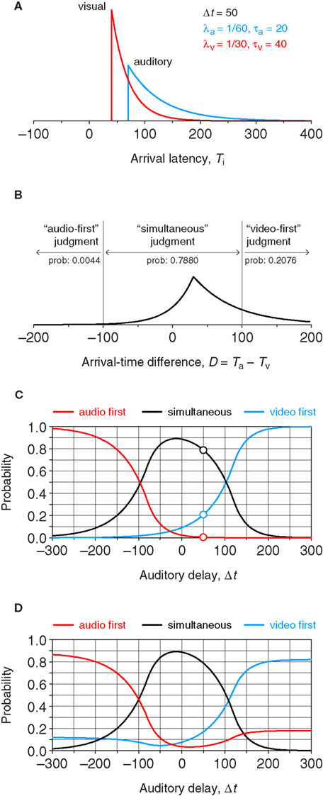
Figure 1. Model of timing judgments. (A) Exponential distributions for the arrival latency of a visual stimulus (red curve) presented at time 0 and an auditory stimulus (blue curve) presented at time Δt = 50 ms. Parameters as indicated. (B) Bilateral exponential distribution of arrival-time differences and boundaries on the decision space (vertical lines, at D = ± δ with δ = 100), determining the probability of each type of judgment. (C). Error-free psychometric functions for each type of response as a function of auditory delay. Circles denote the probabilities indicated in (B) for Δt = 50 ms. (D) Psychometric functions when response errors occur as described in the text.

where τ = τ_a − τ_v. Figure 1B shows the distribution of arrival-time differences for the case in Figure 1A. A resolution parameter δ – which was referred to as threshold by Sternberg and Knoll (1973), Allan (1975), and Ulrich (1987) and as moment duration by Schneider and Bavelier (2003) – limits discriminability so that an AF judgment occurs when D is sufficiently large and negative (D < − δ), a VF judgment occurs when D is sufficiently large and positive (D > δ), and an S judgment occurs when the arrival-time difference is below the resolution limit (−δ ≤ D ≤ δ).

For the example in Figure 1B, where δ = 100, the probability of AF, S, and VF judgments are, respectively, 0.0044, 0.7880, and 0.2076 (as indicated in Figure 1B; see also the circles on the curves of Figure 1C). These probabilities change with auditory delay Δt and Figure 1C shows complete psychometric functions. To obtain them, first note that the cumulative distribution for D is

where f is given byEq. 2. Then,

Clearly, Ψ_VF and Ψ_AF are both monotonic and parallelism holds because Ψ_VF(Δt) = 1 − Ψ_AF(Δt + 2δ), that is, the blue curve in Figure 1C differs from an upside-down reversal of the red curve only by a lateral shift.

Equations 4a–4c give the probabilities of the unobservable AF, S, and VF judgments as a function of auditory delay, but the probabilities of observed AF, S, and VF responses may differ from them. For instance, errors in pressing the response keys make the observer’s response differ from the judgment that was made. In addition, blinks or lapses of attention preclude judgments at all and force the observer to guess a response that may not match the judgment that would have been made in the absence of a lapse. We will refer to these misreports as response errors and lapses, respectively, and we will first describe how to incorporate the former into the model.

Let ε_AF, ε_S, and ε_VF be the probabilities (or error rates) that the observer misreports AF, S, and VF judgments, respectively, as a result of an error in pressing the response keys. These errors may actually differ across the judgments that were made, if only because the layout of the response interface may make the observers more likely to misreport one of the judgments and, in such cases, also more likely to misreport it in a particular form. Since misreporting any given judgment can take two forms (i.e., there are two possible intruding responses), let κ_A-B be the conditional probability of misreporting an A judgment as a B response so that κ_A-C = 1 − κ_A-B is the conditional probability of misreporting an A judgment as a C response. Only three conditional probabilities are free parameters, say, κ_S-AF, κ_VF-AF, and κ_AF-S, because κ_S-VF = 1 − κ_S-AF, κ_VF-S = 1 − κ_VF-AF, and κ_AF-VF = 1 − κ_AF-S. The model incorporating response errors thus becomes

where Ψ_AF, Ψ_S, and Ψ_VF on the right-hand sides are given by Eqs 4a–4c. Figure 1D shows the resultant psychometric functions for an observer with a relatively high error rate whereby VF judgments are misreported as AF responses (ε_VF = 0.18 and κ_VF-AF = 1), a weaker error rate whereby AF judgments are misreported as VF responses (ε_AF = 0.12 and κ_AF-S = 0), and no misreports of S judgments (ε_S = 0). Note that the blue and red curves in Figure 1D are non-monotonic and do not satisfy parallelism (after upside-down reversal). Note also that an absence of errors (i.e., ε_AF = ε_S = ε_VF = 0) renders the model in Eqs 4a–4c, in which responses faithfully indicate judgments.

Equations 4a–4c give the probability of (unobservable) judgments, whereas Eqs 5a–5c give the probabilities of observed responses. Thus, observed responses potentially reflect mixtures of “authentic” judgments and intrusions due to errors upon reporting judgments of other types. We will refer to the weights of the intruding responses in these mixtures as intrusion parameters. For the example in Figure 1D, Eqs 5a–5c become

so that for lack of intrusions from AF and VF judgments and also for lack of intrusion of S judgments into AF and VF responses. In contrast, misses 12% of the authentic AF judgments (which intrude into VF responses) and misses 18% of the authentic VF judgments (which intrude into AF responses).

Our next step to model development considers lapses of attention. These lapses (or blinks, yawns, sneezes, …) obviously occur randomly across trials and independently of the auditory delay at the trial and also independently of the judgment that would have been made in the absence of a lapse. There is a (conceivably small) probability γ that a lapse occurs on some trial and, in such case, an observer can only arbitrarily give AF, S, or VF responses perhaps with some bias. Let β_AF, β_S, and β_VF = 1 − β_AF − β_S be the probabilities of these responses in case of a lapse, where β_AF = β_S = β_VF = 1/3 for an unbiased observer (although unbiased guessing behavior cannot be generally assumed in advance). The model incorporating only lapses and the ensuing (potentially biased) guesses thus becomes

The effect of lapses on the shape of observable psychometric functions can be described without graphical illustration: compared to the psychometric functions in Figure 1C, multiplication by 1 − γ shrinks the range of the functions (i.e., shifts the upper asymptotes of Ψ_AF and Ψ_VF down and also scales Ψ_S down, without affecting the lower asymptotes of any of them) whereas the additive term pushes the functions upwards by a small amount, thus shifting the lower asymptotes upwards.

Now, combining the effects of lapses and response errors into an integrated model is as simple as replacing the unmarked psychometric functions on the right-hand sides of Eqs 7a–7c with the right-hand sides of Eqs 5a–5c, yielding

The effect of lapses in this integrated model is again analogous to that described above, except that the shrunken range and vertical shift occur for the psychometric functions in Figure 1D instead of those in Figure 1C. There are three reasons why we will not consider this integrated model, all of which pertain to the limited utility of modeling lapses. The first one is that the model for lapses in Eqs 7a–7c violates parallelism but not monotonicity: all that is implied when only lapses occur is vertical shrinkage and vertical shift of the psychometric functions and, thus, lapses cannot possibly account for the non-monotonicity observed in some data sets. Second, the integrated model in Eqs 8a–8c is unidentifiable, as lapses and response errors both affect the asymptotes of the psychometric functions in an inextricable way for lack of independent evidence as to how much of the effect found in empirical data is caused by lapses and how much is caused by response errors. Finally, many experiments are designed so as to eliminate the influence of lapses by enabling an additional response key for observers to abort the trial if they missed the stimuli and could not make a judgment. This key is usually programmed so that the trial is placed back in the stack of pending trials for administration at a later time (generally not immediately afterward), and observers are instructed to refrain from using this key if they only were uncertain and wanted to have a second chance. If the commendable precaution to enable such “abort” key is taken, lapses do not need to be modeled at all.

Our decision to use only the model with response errors should not be misconstrued for a denial of the existence of lapses. In the context of our goals in this paper, the potential effects of lapses are absorbed by the error parameters in the model that we will use, and the only consequence is that the estimated values for these parameters cannot be literally interpreted as representing only the probabilities of response errors. This is not a crucial problem, because the relevant parameters in research on prior entry or perception of temporal order are only λ_a, λ_v, τ, and δ; parameters describing errors or lapses are rarely of any theoretical interest and they are included in the model only to improve the accuracy with which the relevant parameters are estimated.

Fitting the Model to Data

Model parameters were estimated for data reported by van Eijk et al. (2008) from an audiovisual SJ3 task carried out by 11 observers. Only results for data from their flash–click stimulus will be presented here, as data from the other stimulus yielded similar outcomes. The visual component of the stimulus was a white disk flashed for 12 ms against a dark background and the auditory component was a 12-ms white-noise burst. Auditory delays ranged from −350 to 350 ms in steps of 50 ms, and 60 trials were administered at each auditory delay.

Model parameters for each observer were sought by maximizing the likelihood equation

where R is the set of empirical responses, θ = (λ_a, λ_v, τ, δ, ε_AF, ε_S, ε_VF, κ_S-AF, κ_VF-AF, κ_AF-S) is the vector of free parameters, {Δt₁, Δt₂, …, Δt_N} is the set of N = 15 auditory delays at which responses were collected, and A_i, S_i, and V_i are the observed counts of AF, S, and VF responses at Δt_i. Equation 9 was maximized using NAG subroutine E04JYF (Numerical Algorithms Group, 1999), which implements a quasi-Newton algorithm for constrained optimization. The parameter space spanned the ranges [1/200, 1] for λ_a and λ_v, the range [−150, 150] for τ, the range [0, 300] for δ, the range [0, 0.8] for ε_AF, ε_S, and ε_VF, and the range [0, 1] for κ_AF-S, κ_S-AF, and κ_VF-AF. Two or three initial values were defined for each parameter, which were evenly spaced within the search space for that parameter. Initial values for each parameter were factorially combined to yield 3⁴ × 2⁶ starting points in the 10-dimensional parameter space and the maximization routine ran for each of these starting points, yielding in each case a vector of estimates and a divergence index. On completion, we took the vector of estimates for which divergence was lowest and the likelihood-ratio statistic G² was computed as a measure of goodness-of-fit because this statistic is the one that maximum-likelihood estimates minimize (Collett, 2003, pp. 87–88). Thus, we estimated parameters and measured the goodness of the fit using the same “currency” (Wichmann and Hill, 2001). The asymptotic distribution of all goodness-of-fit statistics is known to yield inaccurate significance levels when expected frequencies are small (García-Pérez, 1994; García-Pérez and Núñez-Antón, 2001, 2004) and this is a common encounter when fitting psychometric functions. For this reason, significance levels were obtained through parametric bootstrap by simulating 5000 data sets using the estimated parameters for each observer and the same number of auditory delays and trials per delay as in the actual experiment.

Figure 2 shows empirical data and fitted functions for each observer, and also shows a summary panel for average data and average fitted curves for all observers (which we include only because this is the format in which alternative fitted curves were reported by van Eijk et al., 2008). Table 1 lists parameter estimates as well as the value and p-value of the G² statistic for each observer. Perhaps the most salient aspect of Figure 2 is that model curves follow the path of the data accurately, accommodating systematic deviations from monotonicity in AF and VF data. Also, S data (black circles) show symmetric or asymmetric patterns that are well described by the model functions (black curves). Despite the visual quality of the fit, a goodness-of-fit test rejected the model for three observers (stars in Table 1) but these rejections seem spurious, as discussed next. Consider the case of observer 3. The data vary smoothly up to intermediate positive auditory delays, and the model curves follow the path of the data very accurately. Yet, at the four longest positive auditory delays S data (black circles) and VF data (blue circles) appear somewhat noisy, unlike AF data (red circles) at the same auditory delays. Thus, it seems that this observer was occasionally misreporting VF judgments as S responses at long positive auditory delays. It is hard to imagine how an alternative model might produce curves that accommodate the smoothly varying data points on the left and center of the panel and then suddenly wind strangely to also accommodate the stray VF and S data points on the far right. It is even harder to agree to model rejection for observers 4 and 9 (for whom the p-values are also only marginally significant; see Table 1), since model curves follow the path of the data accurately across the panel except for occasional data points that deviate haphazardly from the path of the rest of the data. In all cases, the fitted model does not deviate systematically from the data for any observer but the stray location of some data points sometimes causes statistical rejection. An analysis of residuals identified the data points that caused rejection of the model for each observer, and these points are indicated by arrows in Figure 2. Note that, for observer 3, the only two misfitting data points involving AF and VF responses (indicated with red and blue arrows) imply very small observed frequencies and expected frequencies that are even smaller, a well-known cause of improper model rejections (García-Pérez, 1994; García-Pérez and Núñez-Antón, 2001, 2004).

TABLE 1

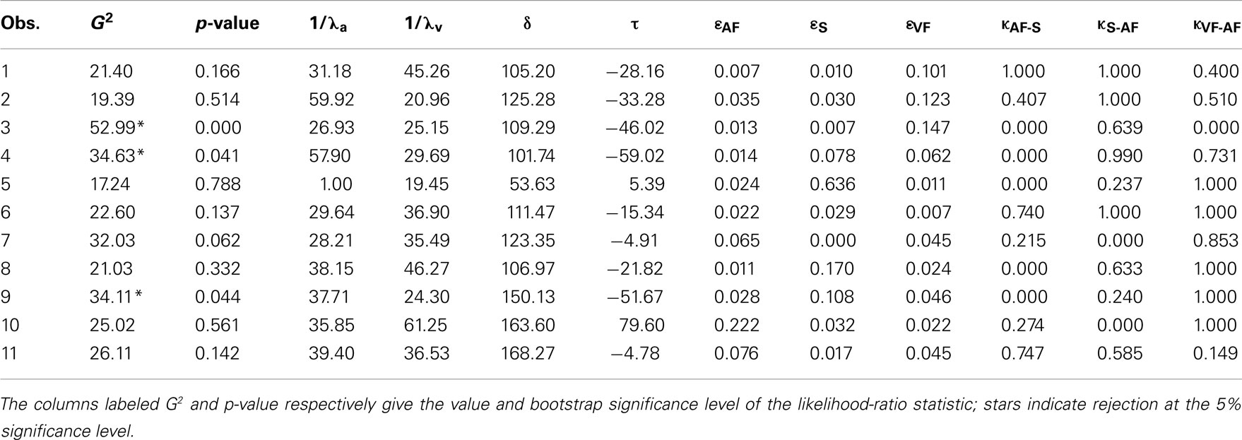
Table 1. Estimated model parameters.

FIGURE 2

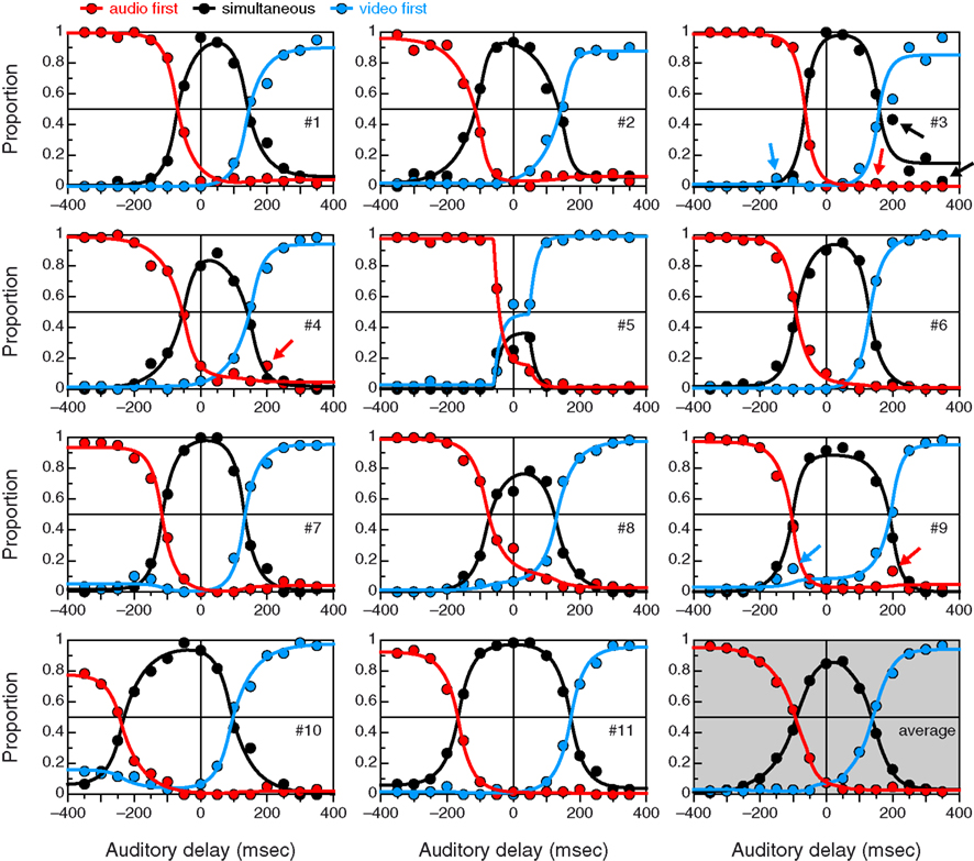
Figure 2. Data and fitted curves in the flash–click experiment of van Eijk et al. (2008). The numeral in each panel denotes the observer; the panel at the bottom right shows summary results as averages of data and averages of the fitted functions across the 11 observers. Arrows in the panels for observers 3, 4, and 9 indicate the data points responsible for the misfit according to a residual analysis.

We do not report sample-wise goodness-of-fit analyses because there is no reason that the model should hold for a given sample as a whole (or just for 95% of the samples when the Type-I error rate is 0.05) but also because analyzing data aggregated across observers poses serious problems (Estes, 1956; Estes and Maddox, 2005). A subject-by-subject analysis of fit seems more reasonable and is the only means for identifying problematic assumptions in a model and potential replacements for them.

Although Figure 2 shows that the model fits the data adequately, we checked for parallelism of VF data (blue symbols) and inverted AF data (red symbols) for each observer, as follows. First, the locations Δt_VF-PSS and Δt_AF-PSS of the 50% point on and were determined. Then, we plotted and thus shifting them so that their 50% points coincide. Finally, we shifted the data analogously and also plotted them (after upside-down reversal of AF data). The results are shown in Figure 3 along with a summary panel for data and curves averaged across observers. The curves only show some deviations from parallelism for observers with relatively high error rates (observers 2, 3, 5, 7, and 10; see Table 1), and these deviations mostly affect the outer ends of each curve, where non-monotonicity also occurs (see Figure 2). It is interesting to note that the data for which Allan (1975) and Ulrich (1987) reported a failure of parallelism also showed non-monotonic patterns at the outer ends, as is expected from intrusions from VF and AF judgments into AF and VF responses. This characteristic is more apparent in the plots that Jaskowski (1991) presented for the same data.

FIGURE 3

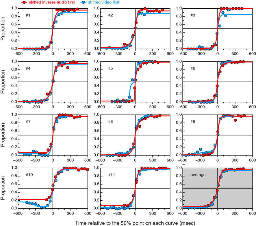
Figure 3. Test of parallelism. In comparison to Figure 2, AF and VF data and curves are merely shifted horizontally (and inverted upside-down in the case of AF data).

A Case of Overfitting?

Overfitting applies to models that have an unnecessarily large number of parameters and, thus, fit data by sheer volume of parameters. All the parameters in our model have empirical referents and, thus, their inclusion is justifiable. Each parameter produces a distinctive and identifiable effect on the shape of the psychometric function, and these effects are not confounded (when lapses and the ensuing guesses are eliminated by design). And, more important, the data to which the model was fitted here show clear signs of these effects, which produce the non-monotonicity and lack of parallelism that conventional models cannot account for.

When considering the risk of overfitting, a comparison with the conventional approach that separately fits arbitrary functions to AF, S, and VF data is enlightening. In particular, on analyzing this same data set, van Eijk et al. (2008) fitted a four-parameter function to AF data, an independent four-parameter function to VF data, and still two other independent three-parameter functions to S data (one of them for the ascending part and the other for the descending part). This yields a total of 14 parameters to describe the same data. Without the simplifications used by van Eijk et al., the number of free parameters under this approach may reach 16. And not only the number of parameters is larger than that implied in our model, the functions fitted in this way cannot produce non-monotonic shapes for AF or VF data and the estimated parameters are uninterpretable in terms of underlying processes: they only indicate the slope, location, and asymptotes of the fitted functions.

Nevertheless, there is still the issue of whether some of the parameters of our model could be disposed of (particularly some of those representing response errors), or whether the simpler model with lapses would suffice to account for the data without response errors. The latter issue can be easily dispatched, as we showed above that a model including only lapses cannot produce non-monotonic psychometric functions for AF and VF data. Since the data actually show these characteristics, the model with only lapses (Eqs 7a–7c) is disproved. To show that overfitting does not affect the model including response errors, we fitted simpler versions of it to the data, as described next.

In the simplest version, response errors are assumed to not occur at all, which implies making ε_AF = ε_S = ε_VF = 0 (wiping out κ_S-AF, κ_VF-AF, and κ_AF-S along the way; see Eqs 5a–5c) and leaving a model with only four free parameters (λ_a, λ_v, τ, and δ). The results are shown in Figure 4, which reveals that forcing model curves to have their asymptotes at 0 or 1 (as applicable) prevent them from accommodating the data, and the fit is particularly bad for observers whose data show clear signs of non-monotonicity or lack of parallelism. The G² statistic rejected the model for all observers (the largest p-value across observers was 0.002), a result that raises no concerns of potentially improper rejections given the obvious mismatch between the path described by the data and the path described by the curves in Figure 4.

FIGURE 4

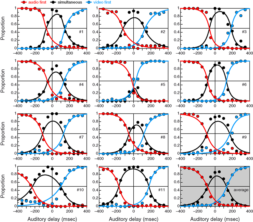
Figure 4. Results of fitting a simpler version of the model in which no response errors are assumed to occur. Layout and graphical conventions as in Figure 2.

In an intermediate version, all response errors were assumed to occur with the same probability (which implies making ε_AF = ε_S = ε_VF = ε) and errors were further assumed to take all possible forms with the same probability (which implies making κ_S-AF = κ_VF-AF = κ_AF-S = 1/2). This renders a model with five parameters (λ_a, λ_v, τ, δ, and ε) for which Figure 5 shows the results. Again, the assumption that all response errors are equally likely prevents the model from fitting data that show clear signs to the contrary: this assumption forces the lower asymptote of all curves to be at the same height, and the upper asymptotes of curves for AF and VF data to also be at the same height, but the data say otherwise. This model was rejected for all observers except 2, 6, and 11, but it does not seem to do justice to the data for observer 2 (see data and curves in the bottom part of the panel for this observer in Figure 5).

FIGURE 5

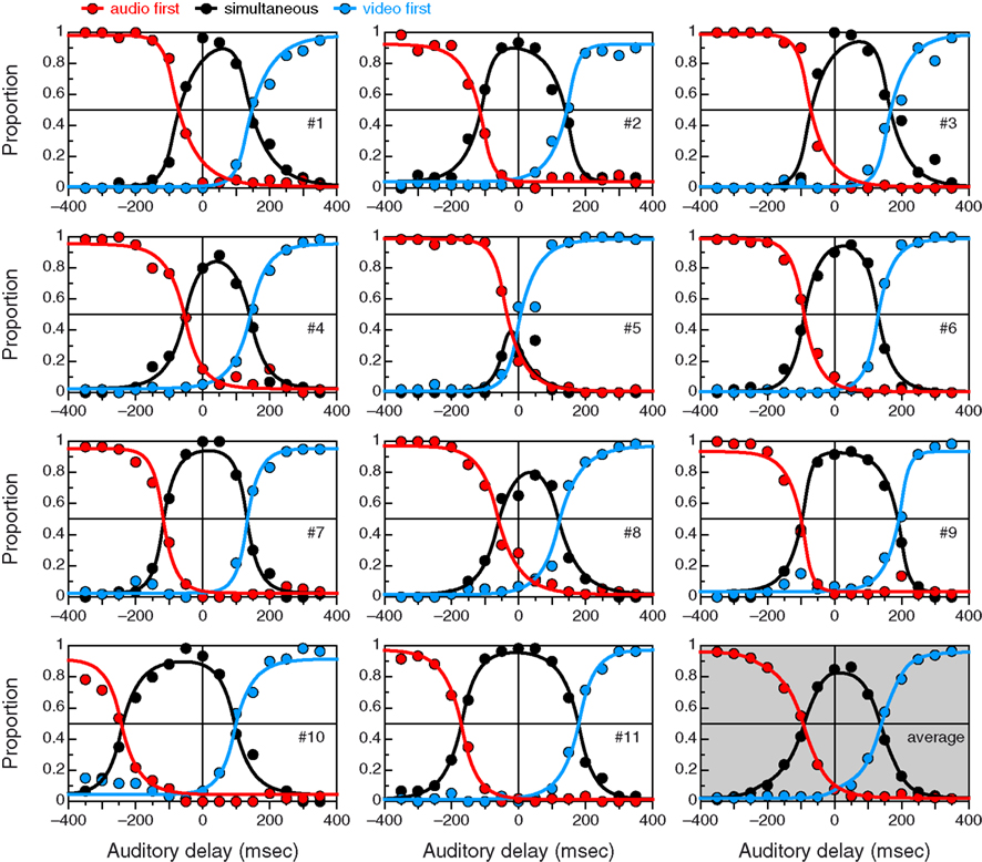
Figure 5. Results of fitting a version of the model in which all types of response error are assumed to occur with the same probability and where the two types of misreported responses in case of error are assumed to occur with the same probability. Layout and graphical conventions as in Figure 2.

We also tried out other simplifications, with analogous outcomes. Although some models fitted the data for some observers, accounting for the diversity of patterns of non-monotonicity and lack of parallelism across observers was impossible without allowance for all parameters. But this allowance does not imply that all parameters were actually useful to fit the data for all observers. Indeed, fitting the full model eliminates unnecessary error parameters by estimating them at or near zero. Consider the data for observer 3 in Figure 2 and note in Table 1 that the estimated values of ε_AF and ε_S are nearly zero, which makes the estimated values of parameters κ_S-AF and κ_AF-S meaningless and immaterial. At the same time, the estimated value of ε_VF is 0.147 with an estimated κ_VF-AF of 0 (or, equivalently, a derived value for κ_VF-S of 1, which are both meaningful because their companion error parameter ε_VF is not null). This matches what the data for observer 3 suggest: only VF judgments seem to be occasionally misreported and always in the form of S responses. A similar analysis for observer 10 reveals the same match between features of the data and interpretation of parameter estimates, with the implicit elimination of unnecessary error parameters and their companion κ’s.

Parameter Identification

Four of the ten free parameters in the model (λ_a, λ_v, τ, and δ) govern judgments and six (ε_AF, ε_S, ε_VF, κ_S-AF, κ_VF-AF, and κ_AF-S) pertain to response errors. This may raise concerns of theoretical identifiability, that is, whether different sets of parameter values may produce the same psychometric functions , and . Since the problem cannot be addressed analytically, we took the approach of determining the extent to which the generating parameters were recovered from data sets essentially implying an infinite number of observations (because sampling error is not of concern here). One-thousand data sets were produced from random combinations of parameters with uniform distributions on [1/80, 1/20] for λ_a and λ_v (independently), on [−80, 80] for τ, on [20, 150] for δ, on [0, 0.1] for ε_AF, ε_S, and ε_VF (independently), and on [0, 1] for κ_AF-S, κ_S-AF, and κ_VF-AF (independently). The particular parameters that would produce each data set were inserted into Eqs 5a–5c and the resultant probabilities at auditory delays ranging from −350 to 350 ms in steps of 50 ms were transformed into (rounded off) expected numbers of AF, S, and VF responses across 10,000 putative trials per auditory delay. The model was subsequently fitted to each data set and parameter estimates were compared with the generating parameters in search for evidence of non-identifiability. The results are shown in Figure 6 in the form of scatter plots of estimated against true parameter values. As is clear, all parameters are recovered with no evidence of non-identifiability. The minor misestimation problems affecting conditional probabilities κ_AF-S, κ_S-AF, and κ_VF-AF (third row in Figure 4) are only a result of the fact that evidence on their actual values is limited or null when ε_AF, ε_S, and ε_VF are very small. The bottom row of Figure 6 shows that this misestimation is not a problem when intrusion parameters are considered.

FIGURE 6

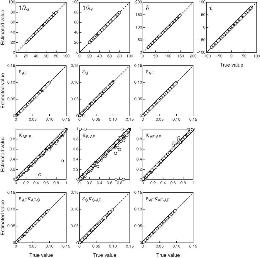
Figure 6. Theoretical parameter identification. Each panel shows a scatter plot of estimated value against true value for the parameter indicated at the top-left corner, including the ten parameters of the model (first three rows) and the derived intrusion parameters (bottom row). Non-identifiability would show as data points falling along lines or curves other than the diagonal identity line in two or more panels within the first three rows.

A related issue is that of practical identifiability, that is, the extent to which model parameters can be recovered accurately from a finite number of observations affected by sampling error. When theoretical identifiability holds, as just documented, lack of practical identifiability speaks more of the scarcity of data than it speaks of the model itself. We looked into this issue under the same conditions discussed in the preceding paragraph (i.e., N = 15 auditory delays and the same ranges of generating parameters), but now using 1000 sets of simulated counts (instead of expected counts) for numbers of trials ranging from 50 to 400 per auditory delay. The accuracy with which parameters were identified was measured through the concordance coefficient (Lin, 1989). The results are shown in Figure 7, which indicates how the concordance coefficient varies with number of trials per auditory delay. The parameters describing perception of temporal order (λ_a, λ_v, τ, and δ; first panel), the error parameters ε_AF and ε_VF (second panel), and the conditional probabilities κ_AF-S and κ_VF-AF (third panel) can be sufficiently accurately recovered with 100 trials per auditory delay. Yet, ε_S and κ_S-AF are harder to recover, a result of the fact that misreports of S judgments (which would occur at short auditory delays) are harder to identify than misreports of AF or VF judgments (which would occur at long positive and negative auditory delays)¹.

FIGURE 7

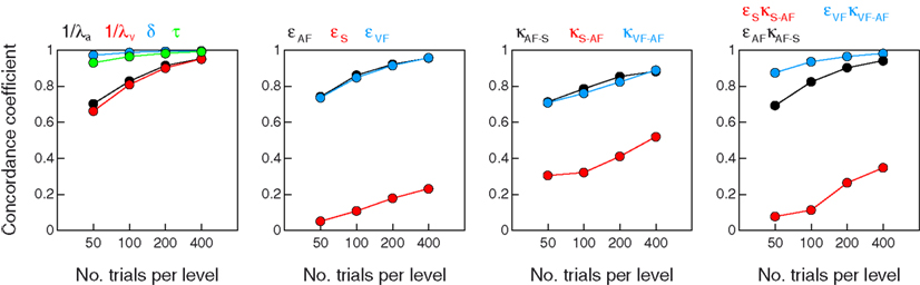
Figure 7. Practical parameter identification. Each panel shows how recovery of the 10 parameters of the model (first three panels) and the derived intrusion parameters (fourth panel) varies with the number of observations collected at each of 15 auditory delays ranging from −350 to 350 ms in steps of 50 ms. An asymptotic 0.05-size chi-square test yielded empirical rejection rates of 4.3, 4.1, 5.4, and 5.5% as the number of observations per auditory delay increased from 50 to 400; an analogous asymptotic 0.05-size likelihood-ratio test yielded inaccurate empirical rejection rates of 8.1, 8.0, 7.3, and 8.3%.

In sum, model parameters are theoretically and practically identifiable with only a slight misestimation of error parameters affecting S judgments, something that does not hamper the estimation of the relevant parameters governing perception of temporal order (λ_a, λ_v, τ, and δ). In any case, error rates are nuisance parameters that are known to be generally difficult to estimate accurately (García-Pérez and Alcalá-Quintana, 2005) but it is also known that including them in the functions to be fitted increases the precision with which relevant parameters can be estimated (see also García-Pérez and Alcalá-Quintana, 2010a,b, 2011). Actually, allowance for error or lapse parameters in model psychometric functions for binary tasks is routine practice in visual psychophysics (Kingdom and Prins, 2010), but not so much in psychoacoustics or in research on prior entry or perception of temporal order. More thorough studies of parameter recovery also involving alternative estimation methods should be carried out, but these lie beyond the scope of this paper.

Conclusion

SJ3 data can be described by independent-channels models when response errors are considered, as lack of monotonicity and parallelism results from these errors. Lapses of attention, in turn, produce lack of parallelism but not lack of monotonicity. Response errors are often made inadvertently and, then, cannot be easily removed from the data. Yet, the contaminating influence of lapses can be easily removed by allowing observers to abort trials in which they missed the stimuli, instead of forcing them to indicate a judgment that they could not possibly have made. Implementing this feature in the response interface is highly recommendable.

Reinstating independent-channels models with their interpretable parameters will contribute to a more precise analysis of the effects of experimental manipulations in studies of prior entry or temporal recalibration. Recourse to these models will also be useful in general studies on the perception of temporal order under different stimulus conditions (see van Eijk et al., 2008, 2010) and for the analysis of observed differences in performance across tasks (i.e., the ternary SJ3 task considered here, its binary version SJ2 in which observers only indicate whether presentation was simultaneous or sequential, and the temporal order judgment task TOJ in which observers are forced to respond AF or VF without allowance for an S response; see García-Pérez and Alcalá-Quintana, submitted).

The model presented here emphasizes the distinction between unobservable judgments and observed responses, where the latter are not direct indicators of the former when response errors occur. Evidence of response errors is conspicuous in empirical data and errors are likely to occur more often when reaction times are also measured, due to the pressure to respond quickly and the ternary nature of the task (i.e., observers have to be quick but without mistaking which of the three response keys they have to press to indicate their judgment). Because response errors are not unlikely in these cases, fitting a model that allows for them is thus of outmost importance in these cases. User-friendly software packages (in MATLAB and R) are under development for fitting the model presented here to SJ3 data (Alcalá-Quintana and García-Pérez, submitted).

Conflict of Interest Statement

The authors declare that the research was conducted in the absence of any commercial or financial relationships that could be construed as a potential conflict of interest.

Acknowledgments

This research was supported by grant PSI2009-08800 from Ministerio de Ciencia e Innovación (Spain). We thank Rob van Eijk for kindly supplying their data. We also thank Michael Lawrence and Mark Yates for their comments on an earlier draft. Correspondence concerning this article should be sent to Miguel A. García-Pérez, Departamento de Metodología, Facultad de Psicología, Universidad Complutense, Campus de Somosaguas, 28223 Madrid, Spain (e-mail: miguel@psi.ucm.es).

Footnote

1. ^For some mixture models, it has been reported that the EM algorithm yields more favorable estimation performance in terms of bias and variability of estimates (e.g., Lawrence, 2010). Checking out whether (and to what extent) the EM algorithm outperforms the quasi-Newton method used here is an area of future research.

References

Allan, L. G. (1975). The relationship between judgments of successiveness and judgments of order. Percept. Psychophys. 18, 29–36.

CrossRef Full Text

Collett, D. (2003). Modelling Binary Data, 2nd Edn. Boca Raton: CRC Press.

Colonius, H., and Diederich, A. (2011). Computing an optimal time window of audiovisual integration in focused attention tasks: illustrated by studies on effect of age and prior knowledge. Exp. Brain Res. 212, 327–337.

Pubmed Abstract | Pubmed Full Text | CrossRef Full Text

Diederich, A., and Colonius, H. (2011). “Modeling multisensory processes in saccadic responses: time-window-of-integration model,” in The Neural Bases of Multisensory Processes, eds M. M. Murray and M. T. Wallace (Boca Raton: CRC Press), 253–276.

Estes, W. K. (1956). The problem of inference from curves based on group data. Psychol. Bull. 53, 134–140.

Pubmed Abstract | Pubmed Full Text | CrossRef Full Text

Estes, W. K., and Maddox, W. T. (2005). Risks of drawing inferences about cognitive processes from model fits to individual versus average performance. Psychon. Bull. Rev. 12, 403–408.

Pubmed Abstract | Pubmed Full Text | CrossRef Full Text

Fujisaki, W., and Nishida, S. (2009). Audio–tactile superiority over visuo–tactile and audio–visual combinations in the temporal resolution of synchrony perception. Exp. Brain Res. 198, 245–259.

Pubmed Abstract | Pubmed Full Text | CrossRef Full Text

García-Pérez, M. A. (1994). Parameter estimation and goodness-of-fit testing in multinomial models. Br. J. Math. Stat. Psychol. 47, 247–282.

CrossRef Full Text

García-Pérez, M. A., and Alcalá-Quintana, R. (2005). Sampling plans for fitting the psychometric function. Span. J. Psychol. 8, 256–289.

Pubmed Abstract | Pubmed Full Text

García-Pérez, M. A., and Alcalá-Quintana, R. (2010a). The difference model with guessing explains interval bias in two-alternative forced-choice detection procedures. J. Sens. Stud. 25, 876–898.

CrossRef Full Text

García-Pérez, M. A., and Alcalá-Quintana, R. (2010b). Reminder and 2AFC tasks provide similar estimates of the difference limen: a reanalysis of data from Lapid, Ulrich, and Rammsayer (2008) and a discussion of Ulrich and Vorberg (2009). Atten. Percept. Psychophys. 72, 1155–1178. [A correction has been published: Atten. Percept. Psychophys. 2012, 74, 489–492.]

CrossRef Full Text

García-Pérez, M. A., and Alcalá-Quintana, R. (2011). Interval bias in 2AFC detection tasks: sorting out the artifacts. Atten. Percept. Psychophys. 73, 2332–2352.

Pubmed Abstract | Pubmed Full Text | CrossRef Full Text

García-Pérez, M. A., and Núñez-Antón, V. (2001). Small-sample comparisons for power-divergence goodness-of-fit statistics for symmetric and skewed simple null hypotheses. J. Appl. Stat. 28, 855–874.

CrossRef Full Text

García-Pérez, M. A., and Núñez-Antón, V. (2004). Small-sample comparisons for goodness-of-fit statistics in one-way multinomials with composite hypotheses. J. Appl. Stat. 31, 161–181.

CrossRef Full Text

Harrar, V., and Harris, L. R. (2008). The effect of exposure to asynchronous audio, visual, and tactile stimulus combinations on the perception of simultaneity. Exp. Brain Res. 186, 517–524.

Pubmed Abstract | Pubmed Full Text | CrossRef Full Text

Heath, R. A. (1984). Response time and temporal order judgement in vision. Aust. J. Psychol. 36, 21–34.

CrossRef Full Text

Jaskowski, P. (1991). Two-stage model for order discrimination. Percept. Psychophys. 50, 76–82.

Pubmed Abstract | Pubmed Full Text | CrossRef Full Text

Jaskowski, P. (1993). Selective attention and temporal-order judgment. Perception 22, 681–689.

Pubmed Abstract | Pubmed Full Text | CrossRef Full Text

Kingdom, F. A. A., and Prins, N. (2010). Psychophysics: A Practical Introduction. London: Academic Press.

Kristofferson, A. B., and Allan, L. G. (1973). “Successiveness and duration discrimination,” in Attention and Performance IV, ed. S. Kornblum (New York: Academic Press), 737–749.

Lawrence, M. A. (2010). Estimating the probability and fidelity of memory. Behav. Res. Methods 42, 957–968.

Pubmed Abstract | Pubmed Full Text | CrossRef Full Text

Lin, L. I.-K. (1989). A concordance correlation coefficient to evaluate reproducibility. Biometrics 45, 255–268.

Pubmed Abstract | Pubmed Full Text | CrossRef Full Text

Nicholls, M. E. R., Lew, M., Loetscher, T., and Yates, M. J. (2011). The importance of response type to the relationship between temporal order and numerical magnitude. Atten. Percept. Psychophys. 73, 1604–1613.

Pubmed Abstract | Pubmed Full Text | CrossRef Full Text

Numerical Algorithms Group. (1999). NAG Fortran Library Manual, Mark 19. Oxford: Numerical Algorithms Group.

Occelli, V., Spence, C., and Zampini, M. (2011). Audiotactile interactions in temporal perception. Psychon. Bull. Rev. 18, 429–454.

Pubmed Abstract | Pubmed Full Text | CrossRef Full Text

Schneider, K. A., and Bavelier, D. (2003). Components of visual prior entry. Cogn. Psychol. 47, 333–366.

Pubmed Abstract | Pubmed Full Text | CrossRef Full Text

Shore, D. I., Spry, E., and Spence, C. (2002). Confusing the mind by crossing the hands. Cogn. Brain Res. 14, 153–163.

CrossRef Full Text

Spence, C., Baddeley, R., Zampini, M., James, R., and Shore, D. I. (2003). Multisensory temporal order judgments: when two locations are better than one. Percept. Psychophys. 65, 318–328.

Pubmed Abstract | Pubmed Full Text | CrossRef Full Text

Spence, C., and Parise, C. (2010). Prior-entry: a review. Conscious. Cogn. 19, 364–379.

Pubmed Abstract | Pubmed Full Text | CrossRef Full Text

Sternberg, S., and Knoll, R. L. (1973). “The perception of temporal order: fundamental issues and a general model,” in Attention and Performance IV, ed. S. Kornblum (New York: Academic Press), 629–685.

Stetson, C., Cui, X., Montague, P. R., and Eagleman, D. M. (2006). Motor-sensory recalibration leads to an illusory reversal of action and sensation. Neuron 51, 651–659.

Pubmed Abstract | Pubmed Full Text | CrossRef Full Text

Stone, J. V., Hunkin, N. M., Porrill, J., Wood, R., Keeler, V., Beanland, M., Port, M., and Porter, N. R. (2001). When is now? Perception of simultaneity. Proc. R. Soc. Lond. B Biol. Sci. 268, 31–38.

CrossRef Full Text

Swanson, W. H., and Birch, E. E. (1992). Extracting thresholds from noisy psychophysical data. Percept. Psychophys. 51, 409–422.

Pubmed Abstract | Pubmed Full Text | CrossRef Full Text

Ulrich, R. (1987). Threshold models of temporal-order judgments evaluated by a ternary response task. Percept. Psychophys. 42, 224–239.

Pubmed Abstract | Pubmed Full Text | CrossRef Full Text

van Eijk, R. L. J., Kohlrausch, A., Juola, J. F., and van de Par, S. (2008). Audiovisual synchrony and temporal order judgments: effects of experimental method and stimulus type. Percept. Psychophys. 70, 955–968.

Pubmed Abstract | Pubmed Full Text | CrossRef Full Text

van Eijk, R. L. J., Kohlrausch, A., Juola, J. F., and van de Par, S. (2010). Temporal order judgment criteria are affected by synchrony judgment sensitivity. Atten. Percept. Psychophys. 72, 2227–2235.

Pubmed Abstract | Pubmed Full Text | CrossRef Full Text

Vatakis, A., Navarra, J., Soto-Faraco, S., and Spence, C. (2008). Audiovisual temporal adaptation of speech: temporal order versus simultaneity judgments. Exp. Brain Res. 185, 521–529.

Pubmed Abstract | Pubmed Full Text | CrossRef Full Text

Vroomen, J., and Keetels, M. (2010). Perception of intersensory synchrony: a tutorial review. Atten. Percept. Psychophys. 72, 871–874.

Pubmed Abstract | Pubmed Full Text | CrossRef Full Text

Wichmann, F. A., and Hill, N. J. (2001). The psychometric function: I. Fitting, sampling, and goodness of fit. Percept. Psychophys. 63, 1293–1313.

Pubmed Abstract | Pubmed Full Text | CrossRef Full Text

Yates, M. J., and Nicholls, M. E. R. (2009). Somatosensory prior entry. Atten. Percept. Psychophys. 71, 847–859.

Pubmed Abstract | Pubmed Full Text | CrossRef Full Text

Yates, M. J., and Nicholls, M. E. R. (2011). Somatosensory prior entry assessed with temporal order judgments and simultaneity judgments. Atten. Percept. Psychophys. 73, 1586–1603.

Pubmed Abstract | Pubmed Full Text | CrossRef Full Text