A Quantum Probability Model of Causal Reasoning

People can often outperform statistical methods and machine learning algorithms in situations that involve making inferences about the relationship between causes and effects. While people are remarkably good at causal reasoning in many situations, there are several instances where they deviate from expected responses. This paper examines three situations where judgments related to causal inference problems produce unexpected results and describes a quantum inference model based on the axiomatic principles of quantum probability theory that can explain these effects. Two of the three phenomena arise from the comparison of predictive judgments (i.e., the conditional probability of an effect given a cause) with diagnostic judgments (i.e., the conditional probability of a cause given an effect). The third phenomenon is a new finding examining order effects in predictive causal judgments. The quantum inference model uses the notion of incompatibility among different causes to account for all three phenomena. Psychologically, the model assumes that individuals adopt different points of view when thinking about different causes. The model provides good fits to the data and offers a coherent account for all three causal reasoning effects thus proving to be a viable new candidate for modeling human judgment.

1. Introduction

People can perform remarkably well at causal reasoning tasks that prove to be extremely difficult for statistical methods and machine learning algorithms. For example, Gopnik et al. (2001) demonstrated that individuals can infer causal relationships even when sample sizes are too small for statistical tests. Further, people can infer hidden causal structures that are difficult for computer scientists or statisticians to uncover (Kushnir et al., 2003). Even though people can infer rich causal representations of the world based on limited data, human causal reasoning is not infallible. Like many other types of subjective probability judgments, judgments about causal events often deviate from the normative rules of classic probability theory. This paper describes a quantum inference model previously developed in Trueblood and Busemeyer (2011) and demonstrates how it can account for judgment phenomena in causal reasoning problems.

The quantum inference model provides a general framework for updating probabilities about a hypothesis given a sequence of information, and it was first developed to account for order effects. One of the oldest and most reliable findings regarding human inference is that the order in which evidence is presented affects the final inference (Hogarth and Einhorn, 1992). For example, a juror’s belief that a criminal suspect is guilty might depend on the order of presentation of the prosecution and defense. More generally, an order effect occurs when a judgment about the probability of a hypothesis given a sequence of information A followed by B, does not equal the probability of the same hypothesis when the given information is reversed, B followed by A. Because of the commutative nature of events in classical probability, order effects are difficult to explain using Bayesian models. Classical probability theory requires p(A ∩ B | H) = p(B ∩ A | H) which according to Bayes rule implies p(H | A ∩ B) = p(H | B ∩ A) (Trueblood and Busemeyer, 2011).

The quantum inference model is based on the axiomatic principles of quantum probability theory. This theory is a generalized approach to probability that relaxes some of the axioms or assumptions of standard probability theory in order to account for violations of the latter. Quantum probability theory is one of many generalized approaches to probability. Specifically, quantum probability theory is a geometric approach using subspaces and projections. Other generalized probability theories include Dempster-Shafer belief function theory (Fagin and Halpern, 1991) and intuitionist probability theory (Narens, 2003).

Models constructed from quantum probability theory do not make assumptions about biological substrates. Rather, quantum probability models provide an alternative mathematical approach for generating theories of how an observer processes information. The quantum approach has been used to account for a number of phenomena in cognitive science including violations of rational decision-making principles (Pothos and Busemeyer, 2009), conjunction and disjunction fallacies (Busemeyer et al., 2011), paradoxes of conceptual combination (Aerts, 2009), bistable perception (Atmanspacher et al., 2004), and interference effects in perception (Conte et al., 2009).

There are at least four reasons for considering a quantum approach to human judgments: (1) human judgment is not a simple read out from a pre-existing or recorded state, instead it is constructed from the current context and question. Quantum probability theory postulates that an individual’s belief state is undetermined before measurement, and it is the process of imposing measurements that forces a resolution of the indeterminacy. (2) Before measurement, cognition behaves more like a wave than a particle allowing for individuals to feel a sense of ambiguity about different belief states simultaneously. According to quantum probability theory, beliefs remain in a superimposed state until a final decision must be reached, which resolves the uncertainty and produces a collapse of the wave to a specific position like a particle. (3) Changes in context produced by one judgment can affect later judgments. Quantum probability theory captures this phenomenon though the notion of incompatibility allowing for one event to disturb and generate uncertainty about another. (4) Cognitive logic does not necessarily obey the rules of classic logic such as the commutative and distributive axioms. Quantum logic is more generalized than classic logic and can model human judgments that do not obey Boolean logic.

1.1. Quantum Inference Model

The quantum inference model was first developed to account for order effects in a number of different problems including medical diagnostic tasks and jury decision-making problems. The following example of a medical inference task (Bergus et al., 1998) is one of the problems accounted for by the model. Physicians (N = 315) were initially informed about a particular woman’s health complaint, and they were asked to estimate the likelihood that she had an infection on the basis of (a) her medical history and findings of the physical exam and (b) laboratory test results, presented in different orders. For one order, the physicians’ initial estimate started out at 0.67; after they had seen the patient’s history and findings of the physical exam, the estimate increased to 0.78; and then after they had also seen the lab test results, it decreased to 0.51. For the other order, the initial estimate again started at 0.67; after they had seen the lab test results, the estimate decreased to 0.44; and then after they also had seen the history and findings of the physical exam, it increased to 0.59. Because the final judgments were significantly different (0.51 versus 0.59, p = 0.03), an order effect is said to have occurred. Specifically, this type of order effect is called a recency effect, because the same evidence had a larger effect when it appeared at the end as opposed to the beginning of the sequence.

The quantum inference model uses the concept of incompatibility to account for order effects. The concept of compatibility is one of the most important new ideas introduced to cognitive science by quantum probability theory. Specifically, the model assumes that different pieces of information can be incompatible in the following sense: The set of feature patterns used to evaluate one piece of information is not shared by the set used to think of another so that no common set of features can be used to evaluate both pieces of information. For example, a physician needs to use knowledge about one set of features concerning a patient’s history and physical exam, and the physician needs to use knowledge about another set of features concerning laboratory tests, but knowledge about all of the combinations from these two sets is not accessible to the physician. Psychologically, this corresponds to adopting different perspectives when evaluating different pieces of information. For example, in the medical inference task, we assume a physician has different representations for beliefs depending on three different points of view: a point of view determined by the woman’s initial health complaint, a point of view determined by the medical history and findings of the physical exam, and a point of view determined by the laboratory test results.

The quantum model is able to account for the medical inference data (Bergus et al., 1998) and also a similar type of data from the domain of jury decision-making (Trueblood and Busemeyer, 2011). In these experiments, subjects read fictitious criminal cases and made a sequence of three judgments for each case: one before the presentation of any evidence, and two more judgments after presentations of evidence by a prosecutor and a defense. For a random half of the cases, the prosecution was presented before the defense, and for the other half, the defense was presented first.

In one version of the experiment (N = 291) the strength of the prosecution and defense was also manipulated. For example, subjects might be asked to judge the probability that a defendant was guilty based on a weak prosecution and a strong defense. Combining the order manipulation with two levels of strength (strong and weak) allowed for eight different order conditions, and as far as we know, this is the largest existing study of order effects on inference. Because of the many different conditions, this experiment provided a rich testing ground for the quantum inference model. Specifically, we compared the quantum inference model to two previously proposed models of order effects from the judgment and decision-making literature. All of the models had the same number of parameters, and the quantum model provided the best fits.

Because the quantum model provides a general way to calculate probabilities in inference problems, it is natural to apply it to situations involving causal reasoning. We begin by describing two recently discovered phenomena in causal reasoning, and illustrate how the model can account for them. Then, we introduce an a priori prediction about order effects which we test and confirm through a new experimental study.

1.2. Predictive and Diagnostic Causal Judgments

There are two possible ways to frame a causal reasoning problem. As formalized by Fernbach et al. (2011), a predictive probability judgment is represented by the conditional probability p(Effect | Cause) and a diagnostic probability judgment is represented by the conditional probability p(Cause | Effect).

Fernbach et al. (2011) illustrate these two different framings through an example about the transmission of a drug-addiction between a mother and a child. More specifically, a predictive causal reasoning problem could be formulated as “A mother has a drug-addiction. How likely is it that her newborn baby has a drug-addiction?” and a diagnostic causal reasoning problem could be formulated as “A newborn baby has a drug-addiction. How likely is it that the baby’s mother has a drug-addiction?”

One recently discovered finding arises from the comparison of predictive and diagnostic judgments when there are strong and weak alternative causes (Fernbach et al., 2011). The drug-addiction scenario described above is an example of a weak alternative causes scenario because there are few alternatives to a child being drug addicted when the mother is not. On the other hand, a strong alternative causes scenario might be one involving the transmission of dark skin from a mother to a child (Fernbach et al., 2011). In such a scenario, a father with dark skin provides a strong alternative to a child having dark skin when the mother does not. The results of experiment 1 by Fernbach et al. (2011) show that subjects are sensitive to the strength of alternative causes when making probability judgments about diagnostic problems but not when making probability judgments about predictive problems. As expected, the probability judgments for diagnostic problems with strong alternative causes (e.g. “A newborn baby has dark skin. How likely is it that the baby’s mother has dark skin?”) are significantly lower than the probability judgments for diagnostic problems with weak alternative causes (e.g. “A newborn baby has a drug-addiction. How likely is it that the baby’s mother has a drug-addiction?”). One might expect that predictive problems with strong alternative causes should produce higher probability judgments than predictive problems with weak alternative causes because alternative causes increase the likelihood that the effect was brought about by different mechanisms (Fernbach et al., 2011). However, the experimental data shows no significant difference between probability judgments for the two types of predictive problems.

A second finding arises from the comparison of predictive and diagnostic judgments in cases where there are full conditionals and no-alternative conditionals (Fernbach et al., 2010). The term full conditional is used to describe situations in which alternative causes are implicit. For example, the following predictive question is a full conditional used in experiment 1 of Fernbach et al. (2010): “Ms. Y has depression. What is the likelihood she presents with lethargy?” The term no-alternative conditional is used to describe situations in which subjects are told that there are no-alternative causes. For example, a no-alternative conditional for the same depression problem might be “Ms. Y has depression. She has not been diagnosed with any other medical or psychiatric disorder that would cause lethargy. What is the likelihood she presents with lethargy?” One might expect that the following two inequalities should hold

$\begin{array}{rcll}& p\left(\text{Effect}|\text{Cause}\right)>p\left(\text{Effect}|\text{Cause},\text{No}\text{Alternative}\text{Causes}\right)& & \text{(1)}\\ & p\left(\text{Cause}|\text{Effect}\right)<p\left(\text{Cause}|\text{Effect},\text{No}\text{Alternative}\text{Causes}\right).& & \text{(2)}\end{array}$

The first inequality is expected because alternative causes should increase the likelihood of an effect. Even though alternative causes are not specifically mentioned in a full conditional, the alternative causes are still present. Thus, the full conditional should be judged as more likely than the no-alternative conditional in predictive problems. On the other hand, the second inequality is expected because alternative causes compete to explain an effect. Thus, the full conditional should be judged as less likely than the no-alternative conditional in diagnostic problems. Experimental results from (Fernbach et al., 2010) show that the probability judgments of subjects obey the second inequality relating to diagnostic reasoning problems but do not obey the first inequality relating to predictive reasoning problems. In the predictive reasoning scenarios, subjects show no significant difference between their probability judgments in full conditional and no-alternative conditional problems.

The two judgment phenomena described here can both be explained by the quantum inference model. Next, we describe the model in the framework of causal reasoning and demonstrate how it can account for the two findings.

2. The Quantum Inference Model of Causal Reasoning

The quantum inference model has been adopted for causal reasoning problems because it provides a general way for updating probabilities about a hypothesis (e.g., the presence of an effect) given a set of information (e.g., different causes for the effect). The quantum model is not at odds with the causal model view set forth by Fernbach et al. (2011) which posits that individuals adopt a representation that approximates the structure of a system and probability judgments arise from this representation. Fernbach et al. (2011) formalize this idea using a causal Bayes net. While the quantum model provides a new way for calculating probabilities, quantum causal graphs can be constructed in a similar manner to causal Bayes nets and could potentially be used as a way to formalize the specific representation used by individuals.

For all of the applications discussed in this paper, the model assumes there is a single effect which can exist (e) or not exist (e) and one or more causes which are either present (p) or absent (a). Based on this assumption there are four possible elementary events that could occur when considering a single effect and a single cause: the effect exists and the cause is present, the effect exists and the cause is absent, the effect does not exist and the cause is present, and the effect does not exist and the cause is absent. In quantum probability theory, the sample space used in classical probability theory is replaced by a Hilbert space (i.e., a complex number vector space). In our framework, the four elementary events are used to define an orthonormal basis for a four dimensional vector space V:

$V=\text{span}\left\{\left|e\wedge p\right.⟩,\left|e\wedge a\right.⟩,\left|ē\wedge p\right.⟩,\left|ē\wedge a\right.⟩\right\}.$(3)

Quantum probability postulates the existence of a unit length state vector |ψ〉∈V representing an individual’s state of belief¹. The belief state |ψ 〉 can be expressed as a linear combination or superposition of the four basis states:

$|\psi ⟩={\omega }_{e,p}\cdot |e\wedge p⟩+{\omega }_{e,a}\cdot |e\wedge a⟩+{\omega }_{ē,p}\cdot |ē\wedge p⟩+{\omega }_{ē,a}\cdot |ē\wedge a⟩.$(4)

The weights such as ω_e,p are called probability amplitudes and determine the belief about a particular elementary event such as e∧p. The belief state vector can be represented by the four amplitudes when the basis for V is treated as the standard basis for $C^4$:

$\begin{array}{l}\psi =\left[\begin{array}{c}{\omega }_{e,p}\\ {\omega }_{e,a}\\ {\omega }_{\overline{e},p}\\ {\omega }_{\overline{e},a}\end{array}\right]\\ =\left[\begin{array}{c}\text{amplitude\hspace{0.17em}for\hspace{0.17em}effect\hspace{0.17em}exist\hspace{0.17em}and\hspace{0.17em}cause\hspace{0.17em}is\hspace{0.17em}present}\\ \text{amplitude\hspace{0.17em}for\hspace{0.17em}effect\hspace{0.17em}exist\hspace{0.17em}and\hspace{0.17em}cause\hspace{0.17em}is\hspace{0.17em}absent}\\ \text{amplitude\hspace{0.17em}for\hspace{0.17em}effect\hspace{0.17em}does\hspace{0.17em}not\hspace{0.17em}exist\hspace{0.17em}and\hspace{0.17em}cause\hspace{0.17em}is\hspace{0.17em}present}\\ \text{amplitude\hspace{0.17em}for\hspace{0.17em}effect\hspace{0.17em}does\hspace{0.17em}not\hspace{0.17em}exist\hspace{0.17em}and\hspace{0.17em}cause\hspace{0.17em}is\hspace{0.17em}absent}\end{array}\right].\end{array}$(5)

Quantum events are defined geometrically as subspaces (e.g., a line or a plane) within this four dimensional space. For example, the event corresponding to the “effect exists” is defined as the subspace L_e = span{|e ∧ p〉,|e ∧ a〉}. Quantum probabilities are computed by projecting |ψ〉 onto subspaces representing events. Projectors for general events are defined in terms of the projectors for elementary events. For example, the projectors for the elementary events e∧p and e∧a are

$P\left(e,p\right)=\left[\begin{array}{cccc}\hfill 1\hfill & \hfill 0\hfill & \hfill 0\hfill & \hfill 0\hfill \\ \hfill 0\hfill & \hfill 0\hfill & \hfill 0\hfill & \hfill 0\hfill \\ \hfill 0\hfill & \hfill 0\hfill & \hfill 0\hfill & \hfill 0\hfill \\ \hfill 0\hfill & \hfill 0\hfill & \hfill 0\hfill & \hfill 0\hfill \\ \hfill \hfill \end{array}\right],P\left(e,a\right)=\left[\begin{array}{cccc}\hfill 0\hfill & \hfill 0\hfill & \hfill 0\hfill & \hfill 0\hfill \\ \hfill 0\hfill & \hfill 1\hfill & \hfill 0\hfill & \hfill 0\hfill \\ \hfill 0\hfill & \hfill 0\hfill & \hfill 0\hfill & \hfill 0\hfill \\ \hfill 0\hfill & \hfill 0\hfill & \hfill 0\hfill & \hfill 0\hfill \\ \hfill \hfill \end{array}\right],$(6)

and the projector for the event the “effect exists” corresponds to the sum of the two projectors: P(e) = P(e,p) + P(e,a). To calculate the probability of this event, the state vector |ψ〉 is projected onto L_e by the projector P_e:

$P\left(e\right)\psi =\left[\begin{array}{cccc}1& 0& 0& 0\\ 0& 1& 0& 0\\ 0& 0& 0& 0\\ 0& 0& 0& 0\end{array}\right]\left[\begin{array}{c}{\omega }_{e,p}\\ {\omega }_{e,a}\\ {\omega }_{\overline{e},p}\\ {\omega }_{\overline{e},a}\end{array}\right]=\left[\begin{array}{c}{\omega }_{e,p}\\ {\omega }_{e,a}\\ 0\\ 0\end{array}\right].$(7)

The probability of the event L_e is equal to the squared length of this projection:

$p\left(L_e\right)={∥P\left(e\right)\psi ∥}^2={∥{\omega }_{e,p}∥}^2+{∥{\omega }_{e,a}∥}^2.$(8)

One of the important differences between quantum probability theory and classical probability theory occurs when multiple events are considered. When multiple events are involved, quantum theory allows for these events to be incompatible. Intuitively, compatibility means that two events X and Y can be accessed simultaneously without interfering with each other. On the other hand, if X and Y are incompatible, they cannot be accessed simultaneously. From a cognitive standpoint, this implies that the two events are processed serially and one interferes with the other. Mathematically, at set of incompatible elementary events are represented by different bases for the same vector subspace. In the case of more general events, consider the event X represented by the subspace L_x with basis |x₁〉, …, |x_n〉 and the event Y represented by the subspace L_y with basis |y₁〉, …, |y_n〉. If the two events are incompatible, then the |x_i〉 basis is a unitary transformation of the |y_i〉 basis. If X and Y are compatible, then there is one basis representation for both events. In this case, quantum probability theory reduces to classic probability theory.

For the purposes of this paper, we assume that the effect is compatible with the causes and multiple causes are incompatible with each other. To formalize this notion, consider a single effect and a single cause (for clarity, call this cause “cause 1”). The basis defined in equation 3 can be used to represent beliefs about the effect and “cause 1.” Now, suppose the same effect is considered in terms of a different cause (call this cause “cause 2”). Because “cause 1” and “cause 2” are incompatible, the four basis elements defined above for “cause 1” cannot be used to describe the relationship between the effect and “cause 2.” This is because incompatible events are represented mathematically by different bases for the same vector space. Thus, a unitary transformation U is applied to the “cause 1” basis to “rotate” it to the “cause 2” basis. The transformation must be unitary to preserve the orthonormal nature of the basis elements. The result of the unitary transformation is a new set of basis elements for V that represents an individual’s point of view associated with “cause 2”:

$V=\text{span}\left\{U|e\wedge p\rangle ,U|e\wedge a\rangle ,U|\overline{e}\wedge p\rangle ,U|\overline{e}\wedge a\rangle \right\}.$(9)

As a point of comparison, a classical probability model for a single effect and two causes would use an eight dimensional sample space because there are two outcomes (e or $\overline{e}$) for the effect and two outcomes (p or a) for each cause. By allowing the causes to be incompatible, the eight dimensional space needed for the classical model is reduced to a four dimensional space in the quantum model. This reduction in dimension becomes even more dramatic when a single effect and n different causes are considered. In this case, the dimension of the sample space for the classical model would be 2ⁿ⁺¹ whereas the quantum model with n incompatible causes continues to use only four dimensions. The vector space V of the quantum model remains four dimensional because the n different causes are accounted for by n different bases for V rather than an increase in the dimension of V². Psychologically, the n different bases correspond to different points of view used when thinking about the existence of an effect and the presence or absence of a cause. Formally, there exists a set of unitary operators used to transform one set of basis vectors to another. This is analogous to rotating the axes in multidimensional scaling (Shepard, 1962; Carroll and Chang, 1970) or multivariate signal detection theory (Rotello et al., 2004; Lu and Dosher, 2008).

In the model, unitary transformations correspond to an individual’s shifts in perspective and relate one point of view (i.e., basis) to another. So far, incompatible events have been described as defining different basis for V. An equivalent way of viewing incompatible events is to fix a basis for V such as the basis given in equation 3 and to transform the state vector |ψ〉 by a unitary operator whenever an incompatible event is being considered. In other words, one can either “rotate” the vector space and leave the state vector fixed or one can “rotate” the state vector and leave the space fixed. In the applications below, the belief state is “rotated” and the basis is fixed.

2.1. Construction of Unitary Matrices

Any unitary matrix can be constructed from the matrix exponential function U = e^−iɸH where H is a Hermitian matrix. (A Hermitian matrix is equal to its own conjugate transpose.) Thus, to construct the unitary operators for the quantum inference model, a Hermitian matrix H first needs to be defined. Following Trueblood and Busemeyer (2011), it is assumed that H is constructed from two components, H = H₁ + H₂.

We begin by describing the construction of a Hermitian matrix for a simple two dimensional problem and extend this to define H₁. Suppose that we have a vector space spanned by two basis vectors |e∧p〉 and |e∧a〉. In our original vector space, this is the subspace corresponding to the event the “effect exists.” Also, we assume that this new space can be viewed from different perspectives and define the unitary matrix U_j to transform one perspective into another. This unitary matrix is constructed from a two dimensional Hermitian matrix W.

Any two dimensional Hermitian matrix can be described as a linear combination of the Pauli matrices:

${\sigma }_x=\left[\begin{array}{cc}\hfill 0\hfill & \hfill 1\hfill \\ \hfill 1\hfill & \hfill 0\hfill \\ \hfill \hfill \end{array}\right];{\sigma }_y=\left[\begin{array}{cc}\hfill 0\hfill & \hfill -i\hfill \\ \hfill i\hfill & \hfill 0\hfill \\ \hfill \hfill \end{array}\right];{\sigma }_z=\left[\begin{array}{cc}\hfill 1\hfill & \hfill 0\hfill \\ \hfill 0\hfill & \hfill -1\hfill \\ \hfill \hfill \end{array}\right].$(10)

We let W be defined as

$W={\alpha }_x\cdot {\sigma }_x+{\alpha }_y\cdot {\sigma }_y+{\alpha }_z\cdot {\sigma }_z.$(11)

Now, we can write the corresponding unitary matrix as

$U_j=e^{-i{\varphi }_{j}W}=e^{-i{\varphi }_j\left({\alpha }_x\cdot {\sigma }_x+{\alpha }_y\cdot {\sigma }_y+{\alpha }_z\cdot {\sigma }_z\right)}.$(12)

where we assume that ${\left({\alpha }_x^2+{\alpha }_y^2+{\alpha }_z^2\right)}^{\frac{1}{2}}=1.$ By applying Euler’s formula we can rewrite the unitary matrix as

$U_j=\text{cos}\left({\varphi }_j\right)\cdot I-i\text{sin}\left({\varphi }_j\right)\cdot \left({\alpha }_x\cdot {\sigma }_x+{\alpha }_y\cdot {\sigma }_y+{\alpha }_z\cdot {\sigma }_z\right)$(13)

where I is the 2 × 2 identity matrix. (Euler’s formula states that eⁱɸ = cos(ɸ) + isin(ɸ).) Equation 13 can be written as the matrix

$U_j=\left[\begin{array}{cc}\hfill \text{cos}\left({\varphi }_j\right)-i\cdot {\alpha }_z\cdot \text{sin}\left({\varphi }_j\right)\hfill & \hfill -\left(i\cdot {\alpha }_x+{\alpha }_y\right)\cdot \text{sin}\left({\varphi }_j\right)\hfill \\ \hfill -\left(i\cdot {\alpha }_x-{\alpha }_y\right)\cdot \text{sin}\left({\varphi }_j\right)\hfill & \hfill \text{cos}\left({\varphi }_j\right)+i\cdot {\alpha }_z\cdot \text{sin}\left({\varphi }_j\right)\hfill \\ \hfill \hfill \end{array}\right].$(14)

From equation 14, the unitary matrix U_j produces a rotation of degree ɸ_j around the unit length vector (α_x,α_y,α_z,). (Please see Sakurai, 1994 for more details.) The Hermitian matrix W is said to be a generator for U_j because for small values of ɸ_j, the unitary matrix is approximately equal to 1 − iɸ_jW. (Please see Nielsen and Chuang, 2000, Chapter 4 for more details.)

After applying the matrix U_j, the probability that e ∧ p is true is periodic in the variable ɸ_j. If we want to ensure that p is favored throughout the presentation of the cause, then we must maintain a probability greater than 0.5 for p over a. In the model, the probability for p over a is maximized whenever α_y= 0 and α_x= α_z> 0. By setting α_y= 0, we avoid reversing the preference for p across time. The condition that α_x= α_z> 0 restricts probabilities for p to oscillate back and forth from 0.5 to 1.0 across time. Because the vector (α_x, α_y, α_z) has unit length, we must set ${\alpha }_x={\alpha }_z=\frac{1}{\sqrt{2}}.$ Now, define W as

$W=\frac{1}{\sqrt{2}}\left[\begin{array}{cc}\hfill 1\hfill & \hfill 1\hfill \\ \hfill 1\hfill & \hfill -1\hfill \\ \hfill \hfill \end{array}\right]$(15)

and the 2 × 2 unitary matrix as

$U_j=\text{exp}\left\{-i{\varphi }_j\frac{1}{\sqrt{2}}\left[\begin{array}{cc}\hfill 1\hfill & \hfill 1\hfill \\ \hfill 1\hfill & \hfill -1\hfill \\ \hfill \hfill \end{array}\right]\right\}.$(16)

In the full four dimensional model, we specify the matrix H₁ in terms of the matrix W. Specifically, we assume that H₁ is the tensor product given by

$\begin{array}{rcll}{H}_1& =\left[\begin{array}{cc}\hfill 1\hfill & \hfill 0\hfill \\ \hfill 0\hfill & \hfill 1\hfill \\ \hfill \hfill \end{array}\right]\otimes W=\left[\begin{array}{cc}\hfill 1\hfill & \hfill 0\hfill \\ \hfill 0\hfill & \hfill 1\hfill \\ \hfill \hfill \end{array}\right]\otimes \frac{1}{\sqrt{2}}\left[\begin{array}{cc}\hfill 1\hfill & \hfill 1\hfill \\ \hfill 1\hfill & \hfill -1\hfill \\ \hfill \hfill \end{array}\right]& & \\ & =\frac{1}{\sqrt{2}}\left[\begin{array}{cccc}\hfill 1\hfill & \hfill 1\hfill & \hfill 0\hfill & \hfill 0\hfill \\ \hfill 1\hfill & \hfill -1\hfill & \hfill 0\hfill & \hfill 0\hfill \\ \hfill 0\hfill & \hfill 0\hfill & \hfill 1\hfill & \hfill 1\hfill \\ \hfill 0\hfill & \hfill 0\hfill & \hfill 1\hfill & \hfill -1\hfill \\ \hfill \hfill \end{array}\right].& & \text{(17)}\end{array}$

A unitary matrix with H₁ as a generator transforms the amplitudes toward the presence of causes by rotating the probability amplitudes to favor events involving the “cause is present.” In other words, the corresponding unitary matrix strengthens the amplitudes corresponding to p and weakens the amplitudes corresponding to a. Further, the unitary matrix corresponding to H₁ strengthens and weakens the amplitudes for causes to the greatest extent possible. This results from the fact that the matrix W was designed to maximize the probability of one type of information over another.

Next, we turn to the construction of the H₂ component of the Hermitian matrix H. As with H₁, we begin by defining a Hermitian matrix for a two dimensional space and then extend this to the four dimensional case. Consider the vector space spanned by the basis vectors |e∧p〉 and |ē ∧ p〉. This is the subspace of the full four dimensional vector space corresponding to the presence of a cause. We proceed exactly as before and define a Hermitian matrix V as a linear combination of Pauli matrices. Because we wish to maintain an overall probability greater than 0.5 for the existence or non-existence of an effect across time, we set α_y= 0 and ${\alpha }_x={\alpha }_z=\frac{1}{\sqrt{2}}.$ Thus, we have V = W.

In order to easily write H₂ in terms of V, we rearrange the coordinate vector given in equation 5 so that

$\psi =\left[\begin{array}{c}{\omega }_{e,p}\\ {\omega }_{\overline{e},p}\\ {\omega }_{\overline{e},a}\\ {\omega }_{e,a}\end{array}\right].$(18)

Now we have

$\begin{array}{rcll}{H}_2& =\left[\begin{array}{cc}\hfill 1\hfill & \hfill 0\hfill \\ \hfill 0\hfill & \hfill 1\hfill \\ \hfill \hfill \end{array}\right]\otimes V=\left[\begin{array}{cc}\hfill 1\hfill & \hfill 0\hfill \\ \hfill 0\hfill & \hfill 1\hfill \\ \hfill \hfill \end{array}\right]\otimes \frac{1}{\sqrt{2}}\left[\begin{array}{cc}\hfill 1\hfill & \hfill 1\hfill \\ \hfill 1\hfill & \hfill -1\hfill \\ \hfill \hfill \end{array}\right]& & \\ & =\frac{1}{\sqrt{2}}\left[\begin{array}{cccc}\hfill 1\hfill & \hfill 1\hfill & \hfill 0\hfill & \hfill 0\hfill \\ \hfill 1\hfill & \hfill -1\hfill & \hfill 0\hfill & \hfill 0\hfill \\ \hfill 0\hfill & \hfill 0\hfill & \hfill 1\hfill & \hfill 1\hfill \\ \hfill 0\hfill & \hfill 0\hfill & \hfill 1\hfill & \hfill -1\hfill \\ \hfill \hfill \end{array}\right].& & \text{(19)}\end{array}$

Because we want to combine H₁ and H₂, we will need to use the same arrangement of coordinates for both matrices. To define H₂ in terms of the coordinates given in equation 5, we first switch row two with row three and column two with column three. Next, we switch row two with row four and column two with column four. The resulting matrix is

$H_2=\frac{1}{\sqrt{2}}\left[\begin{array}{cccc}\hfill 1\hfill & \hfill 0\hfill & \hfill 1\hfill & \hfill 0\hfill \\ \hfill 0\hfill & \hfill -1\hfill & \hfill 0\hfill & \hfill 1\hfill \\ \hfill 1\hfill & \hfill 0\hfill & \hfill -1\hfill & \hfill 0\hfill \\ \hfill 0\hfill & \hfill 1\hfill & \hfill 0\hfill & \hfill 1\hfill \\ \hfill \hfill \end{array}\right].$(20)

The Hermitian matrix H₂ evolves an individual’s beliefs about an effect and the presence or absence of a cause. Specifically, it results in transforming amplitudes toward the event the “effect exists and cause is present” and toward the event the “effect does not exist and cause is absent.” As in the case of H₁, the unitary matrix corresponding to H₂ evolves the amplitudes to the greatest extent possible.

Now, we define the Hermitian matrix H as

$\begin{array}{rcll}H& =\frac{1}{\sqrt{2}}\left(\left[\begin{array}{cccc}\hfill 1\hfill & \hfill 1\hfill & \hfill 0\hfill & \hfill 0\hfill \\ \hfill 1\hfill & \hfill -1\hfill & \hfill 0\hfill & \hfill 0\hfill \\ \hfill 0\hfill & \hfill 0\hfill & \hfill 1\hfill & \hfill 1\hfill \\ \hfill 0\hfill & \hfill 0\hfill & \hfill 1\hfill & \hfill -1\hfill \\ \hfill \hfill \end{array}\right]+\left[\begin{array}{cccc}\hfill 1\hfill & \hfill 0\hfill & \hfill 1\hfill & \hfill 0\hfill \\ \hfill 0\hfill & \hfill -1\hfill & \hfill 0\hfill & \hfill 1\hfill \\ \hfill 1\hfill & \hfill 0\hfill & \hfill -1\hfill & \hfill 0\hfill \\ \hfill 0\hfill & \hfill 1\hfill & \hfill 0\hfill & \hfill 1\hfill \\ \hfill \hfill \end{array}\right]\right)& & \\ & =\frac{1}{\sqrt{2}}\left[\begin{array}{cccc}\hfill 2\hfill & \hfill 1\hfill & \hfill 1\hfill & \hfill 0\hfill \\ \hfill 1\hfill & \hfill -2\hfill & \hfill 0\hfill & \hfill 1\hfill \\ \hfill 1\hfill & \hfill 0\hfill & \hfill 0\hfill & \hfill 1\hfill \\ \hfill 0\hfill & \hfill 1\hfill & \hfill 1\hfill & \hfill 0\hfill \\ \hfill \hfill \end{array}\right].& & \text{(21)}\end{array}$

In the sum H₁ + H₂, the H₂ matrix affects the relation between causes and effects and the H₁ matrix biases the amplitudes toward the presence of causes. Both matrices are necessary components of H. The Hermitian matrix, H, was previously developed for psychological applications involving four dimensional vector spaces (Pothos and Busemeyer, 2009) and is identical to the one used in Trueblood and Busemeyer (2011). The parameter ɸ determines the degree of rotation and is used as a free parameter in the model. A different parameter value of ɸ is used for different causes. For more details about the derivation of the unitary operators, please see Pothos and Busemeyer (2009) and Trueblood and Busemeyer (2011).

3. Modeling the Predictive and Diagnostic Phenomena

Now that we have introduced the model, we illustrate how it can be applied to the two findings by Fernbach et al. (2010, 2011) concerning predictive and diagnostic judgments.

3.1. Predictive and Diagnostic Judgments with Strong and Weak Alternative Causes

In experiment 1 conducted by Fernbach et al. (2011), 180 subjects provided probability judgments for predictive and diagnostic reasoning problems with strong and weak alternatives causes. In the experiment, twenty different question categories were used. These categories ranged from mothers and newborn babies to oxygen tanks and scuba divers. For each question category, there were two types of causes – one with strong alternatives and one with weak alternatives. In analyzing the data, Fernbach et al. (2011) averaged over the different categories. Because a large number of categories were used, any differences in the events themselves should average out.

To model data from this experiment, the quantum inference model assumes that equal weight is initially placed on the four elementary events defining the belief state in a manner similar to setting a uniform prior in a Bayesian model:

${\psi }_0=\left[\begin{array}{c}{\omega }_{e,p}\\ {\omega }_{e,a}\\ {\omega }_{\overline{e},p}\\ {\omega }_{\overline{e},a}\end{array}\right]=\left[\begin{array}{c}\sqrt{.25}\\ \sqrt{.25}\\ \sqrt{.25}\\ \sqrt{.25}\end{array}\right].$(22)

The original version of the quantum inference model (Trueblood and Busemeyer, 2011) was applied to inference problems involving a single hypothesis and two pieces of evidence. In this setting, it was assumed an individual adopted three different points of view throughout the inference problem: a point of view determined by the initial description of the problem, a point of view determined by the first piece of evidence, and a point of view determined by the second piece of evidence. A “rotation” of the belief state occurred whenever there was a shift in perspective. In an analogous manner, we assume here that there is a change in perspective (i.e., “rotation”) between the initial point of view, the point of view associated with one of the causes, and the point of view associated with the other cause.

For predictive problems, the initial belief state is revised after an individual learns about the presence of a cause. Psychologically, the new information about the cause results in the individual shifting his or her perspective of the four elementary events. Mathematically, the initial belief state |ψ₀〉 changes to a new state by using a unitary operator to “rotate” the initial belief state: U|ψ₀〉. Because the individual learns the cause is present, the new state is then projected onto the “cause is present” subspace and is normalized to ensure that the length of the new belief state equals one:

$\left|{\psi }_1\right.⟩=\frac{\left(P\left(e,p\right)+P\left(ē,p\right)\right)U|{\psi }_0⟩}{∥\left(P\left(e,p\right)+P\left(ē,p\right)\right)U|{\psi }_0⟩∥}.$(23)

The predictive probability is calculated by projecting the revised belief state onto the “effect exists” subspace and finding the squared length of the projection:

$p\left(\text{Effect}|\text{Cause}\right)={∥P\left(e\right)|{\psi }_1⟩∥}^2.$(24)

For diagnostic problems, the initial belief state is revised after an individual learns the effect exists. In this case, the initial belief state |ψ₀〉 does not need to be transformed by a unitary operator before it is projected onto the “effect exists” subspace. Because we are concerned with only a single effect, there is no need to change perspective between the initial belief state and the belief state associated with the knowledge that the effect is present³. In other words, the initial basis was chosen to describe a single effect being considered in the problem. Thus, the initial state is projected directly onto this subspace and is normalized resulting in a new belief state:

${\psi }_1=\left[\begin{array}{c}{\omega }_{e,p}\\ {\omega }_{e,a}\\ {\omega }_{\overline{e},p}\\ {\omega }_{\overline{e},a}\end{array}\right]=\left[\begin{array}{c}\sqrt{.5}\\ \sqrt{.5}\\ 0\\ 0\end{array}\right].$(25)

The diagnostic probability is calculated by projecting the revised belief state onto the “cause is present” subspace and finding the squared length of the projection. However, before projection, |ψ₁〉 is transformed by a unitary operator to account for the assumed incompatibility between the individual’s current point of view and the point of view associated with the cause:

$p\left(\text{Cause}|\text{Effect}\right)={∥P\left(c\right)U|{\psi }_1⟩∥}^2.$(26)

Because different causes are used in the weak and strong alternative causes problems (e.g. “A mother has a drug-addiction” versus “A mother has dark skin”), different parameter values of ɸ are used. Specifically, one value of ɸ is used to account for causes where the alternatives are weak and another value of ɸ is used to account for causes where the alternatives are strong. Equivalently, different causes are incompatible and thus different unitary operators are needed to “rotate” the state vector. All of the calculations presented here and for the other effects discussed below are also given in appendix B.

The important difference between predictive and diagnostic calculations is the ordering of projections and rotations. In the predictive case, the initial belief state is first rotated by the U matrix and then projected onto the “cause is present” subspace. In the diagnostic case, the initial state is first projected onto the “effect exists” subspace and then rotated by the U matrix. The model predicts that strong and weak alternative causes do not affect predictive judgments because the differences between these two situations, which are incorporated in the rotations, are wiped out by subsequent projections. This is not the case for diagnostic judgments because rotations occur after projections.

The model was fit to the mean judgments for the following four situations: predictive with weak alternative causes, predictive with strong alternative causes, diagnostic with weak alternative causes, and diagnostic with strong alternative causes. The model used two free parameters associated with the two different types of alternative causes (i.e., strong and weak) to model the four judgments. The model was fit by minimizing the sum of the squared error (SSE) between the experimental data and model predictions. The best fit parameters were ɸ₁ = − 3.74 for strong alternative causes and ɸ₂ = 0.48 for the weak alternative causes. Table 1 shows the experimental results and the best fitting model predictions. The mean squared error (MSE) for the model fit was less than 0.0005.

TABLE 1

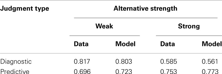
Table 1. Model fits for predictive and diagnostic judgments with strong and weak alternative causes.

Next we show that the same quantum principles also account for the differences between predictive and diagnostic judgments in the more complex paradigm involving the no-alternative conditions.

3.2. Predictive and Diagnostic Judgments with Full and No-Alternative Conditionals

In experiment 1 conducted by Fernbach et al. (2010), 265 mental health practitioners provided probability judgments for predictive and diagnostic reasoning problems with full and no-alternative conditionals related to a scenario about a woman experiencing lethargy given she was diagnosed with depression.

To model this data, many of the same steps described above are used. Specifically, the probabilities for predictive and diagnostic reasoning problems with full conditionals are calculated in the exact same manner as above in equations 24 and 26 respectively.

To calculate the probabilities for predictive and diagnostic reasoning problems with no-alternative conditionals, it is assumed that an individual considers two causes when producing judgments. The first cause is the one explicitly given in the problem (i.e., the woman has been diagnosed with depression). The second cause is implicitly defined in the problem through the statement that there are no-alternative causes (i.e., the woman has not been diagnosed with any other medical or psychiatric disorders that cause lethargy). In keeping with the assumption that all causes are incompatible, these two causes are treated as such. Thus, two different unitary operators, U₁ and U₂ associated with the explicit present cause and the implicit absent cause respectively, are used when revising the belief state.

For predictive problems with the no-alternative conditional, the initial belief state given in equation 22 is first revised after an individual processes information about the presence of the explicit cause. The explicit cause is assumed to be processed first because it is more readily available. The initial state vector is updated according to equation 23 where U is defined as U₁. Next, the new state vector |ψ₁〉 is revised after the individual processes the information about the absence of the implicit cause. Because the two causes are incompatible, the current belief state |ψ₁〉 is changed to a new state by the unitary operator U₂. The new state is then projected onto the “cause is absent” subspace and normalized:

$\left|{\psi }_2\right.⟩=\frac{\left(P\left(e,a\right)+P\left(ē,a\right)\right)U_2\left|{\psi }_1⟩\right.}{∥\left(P\left(e,a\right)+P\left(ē,a\right)\right)U_2\left|{\psi }_1⟩\right.∥}.$(27)

The predictive probability is then calculated by projecting the revised belief state onto to the “effect exists” subspace and finding the squared length of the projection:

$p\left(\text{Effect}|\text{Cause},\text{No}\text{Alternative}\text{Causes}\right)={∥P\left(e\right)|{\psi }_2⟩∥}^2.$(28)

For diagnostic problems with the no-alternative conditional, the initial belief state given in equation 22 is revised to the state given in equation 25 after an individual learns the effect exists. Next, the state undergoes revision when the individual considers information about the implicit cause being absent:

$\left|{\psi }_2\right.⟩=\frac{\left(P\left(e,a\right)+P\left(ē,a\right)\right)\left.U_2\right|{\psi }_1⟩}{∥\left(P\left(e,a\right)+P\left(ē,a\right)\right)\left.U_2\right|{\psi }_1⟩∥}.$(29)

The diagnostic probability is calculated by projecting the belief state |ψ₂〉 onto to the “cause is present” subspace and finding the squared length of the projection. However, before projection, |ψ₂〉 is transformed by the unitary operator U₁ to account for the assumed incompatibility between the individual’s current point of view and the point of view associated with the explicit cause:

$p\left(\text{Cause}|\text{Effect},\text{No}\text{Alternative}\text{Causes}\right)={∥P\left(c\right)U_1|{\psi }_2⟩∥}^2.$(30)

The model was fit to the mean judgments for the following four situations: predictive with full conditional, predictive with no-alternative conditional, diagnostic with full conditional, and diagnostic with no-alternative conditional. The model used two free parameters associated with the two unitary operators used for the two different types of causes (i.e., explicit and implicit). The model was fit by minimizing the sum of the squared error (SSE) between the experimental data and model predictions. The best fit parameters were ɸ₁ = − 2.35 for the explicit cause and ɸ₂ = − 3.81 for the implicit cause. Table 2 shows the experimental results and the best fitting model predictions. The MSE for the model fit was less than 0.0003.

TABLE 2

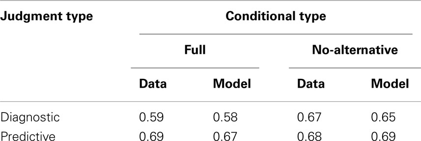
Table 2. Model fits for predictive and diagnostic judgments with full and no-alternative conditionals.

In summary, the quantum model uses the same principles to provide accurate fits to the results from both experiments. However, two parameters were used to fit four data points in each study. Obviously a stronger test of the assumptions underlying the quantum model is required before this account becomes very convincing.

4. Order Effects in Causal Reasoning

So far, the quantum inference model has been based on the assumption that causes are incompatible. This is the key assumption required to account for the findings. The current study was designed to gather experimental support for this assumption. If all events are compatible, then quantum probability theory reduces to classic probability theory. In particular, the events obey the commutative property of Boolean algebra. In a simple Bayesian inference model, the commutative nature of events implies order effects do not occur (Trueblood and Busemeyer, 2011). However, incompatible events do not have to obey the commutative property and can produce order effects. Thus, the quantum inference model with incompatible causes makes an a priori prediction that order effects exist in causal reasoning. The present study tests this prediction.

Subjects in the study were 113 undergraduate students at Indiana University who received experimental credit for introductory psychology courses. Each of the subjects completed a computer-controlled experiment where they read ten different randomized scenarios involving an effect and two causes with one the causes being present and the other cause being absent. For example, subjects might be asked about the likelihood that a high school cafeteria will serve healthier food next month (the effect) given the food budget remains the same (the absent cause) and a group of parents working to fight childhood obesity contacted the school about including healthier menu options (the present cause). All ten scenarios used in the experiment are given in appendix A.

The participants reported the likelihood of the effect on a 0–100 scale before reading either cause, after reading one of the causes, and again after reading the remaining cause. For a random half of the scenarios, subjects judged the present cause before the absent cause. For the remaining half of the scenarios, the subjects judged the absent cause before the present cause. The data was analyzed by collapsing across all ten scenarios. Figure 1 shows the average probability judgments collapsed across the scenarios for the different orderings of the causes. A two sample t-test showed a significant recency effect (t = 9.6408, df = 1128, p < 0.0001). This implies that the second cause influenced subjects’ beliefs more than the first cause. One might think that order effects are due to memory recall failures; however, memory recall is uncorrelated with order effects in sequential judgments (Hastie and Park, 1986).

FIGURE 1

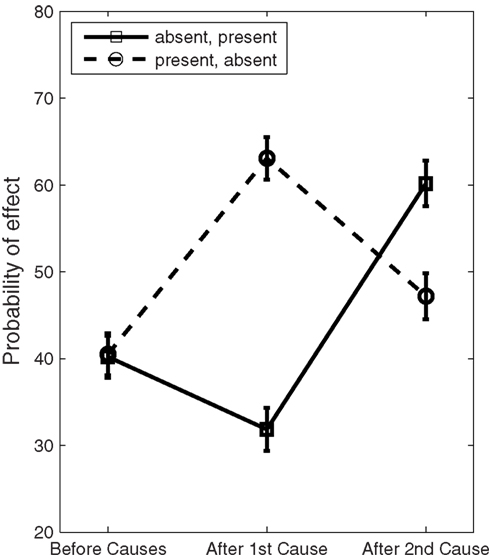
Figure 1. Average probability judgments collapsed across 10 scenarios for two orderings of present and absent causes. The judgments exhibit a significant recency effect as illustrated by the crossing of the two curves on the graph. Error bars show the 95% confidence interval.

The quantum model accounts for the order effect data in a manner similar to its account of predictive judgments with no-alternative conditionals. Specifically, there are two incompatible causes with one being present and the other being absent. Two different unitary operators, U₁ and U₂, are associated with the two causes respectively.

To start, the initial belief state is based on the probability judgments provided by subjects before either cause was presented. The mean probability of the effect given no causal information was 0.403. Thus, the initial state is defined as

${\psi }_0=\left[\begin{array}{c}{\omega }_{e,p}\\ {\omega }_{e,a}\\ {\omega }_{\overline{e},p}\\ {\omega }_{\overline{e},a}\end{array}\right]=\left[\begin{array}{c}\sqrt{\frac{0.403}{2}}\\ \sqrt{\frac{0.403}{2}}\\ \sqrt{\frac{0.597}{2}}\\ \sqrt{\frac{0.597}{2}}\end{array}\right].$(31)

When modeling judgments for the present cause followed by judgments for the absent cause, the initial belief state is first revised to accommodate the information about the present cause. Specifically, the initial state vector is updated according to equation 23 where U is defined as U₁. The probability of the effect given the present cause is calculated as in equation 24. Next, the new state vector |ψ₁〉 is revised after the individual processes the information about the absent cause. This updating occurs according to equation 27. The final probability of the effect given the present cause followed by the absent cause is calculated as in equation 28. To model the judgments for the reverse order of causes, absent cause followed by present cause, a similar set of steps are followed except that the roles of U₁ and U₂ were reversed (U₂ was applied first and U₁ second). It should be noted that the quantum model can produce both primacy and recency effects, and that these two effects oscillate across different values for the phi parameters.

The model was fit to the following four data points: p(Effect | Present Cause), p(Effect | Present Cause, Absent Cause), p(Effect | Absent Cause), p(Effect | Absent Cause, Present Cause). The model used two free parameters associated with the two unitary operators used for the two different types of causes (i.e., present and absent). The model was fit by minimizing the sum of the squared error (SSE) between the experimental data and model predictions. The best fit parameters were ɸ₁ = 3.67 for the present cause and ɸ₂ = − 1.57 for the absent cause. Table 3 shows the experimental results and the best fitting model predictions. The MSE for the model fit was less than 0.0002.

TABLE 3

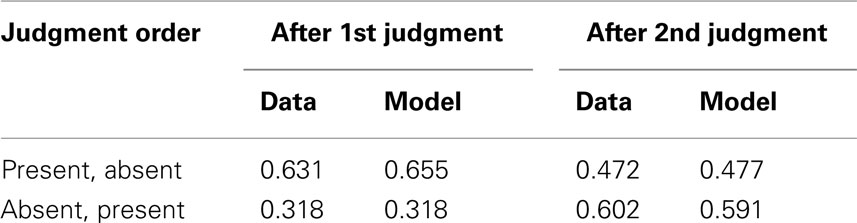
Table 3. Model fits for order effects in predictive judgments.

The existence of order effects provides support for the quantum inference model with incompatible causes. More importantly, the model has introduced a new direction for empirical study not considered before in causal reasoning.

5. Alternative Models

Two other models of inference are worth mentioning. The first model is a causal Bayes net discussed in Fernbach et al. (2011). This model assumes that the relationship between causes and effects can be represented by a directed graph and probabilities are calculated from this structure. The second model is the belief-adjustment model developed by Hogarth and Einhorn (1992). This is an arithmetic model which assumes that beliefs are determined through an anchoring and adjustment process. While both models provide insights into the process of updating beliefs, neither model can provide an adequate account for all three causal reasoning phenomena.

5.1. Causal Bayes Net

Fernbach et al. (2011) present a causal Bayes net as a possible account of predictive and diagnostic judgments with strong and weak alternative causes. In this model, the predictive probability of an effect given a cause is calculated using the noisy-or equation:

$p\left(\text{Effect}|\text{Cause}\right)=W_c+W_a-W_c{W}_a$(32)

where W_c= p(Effect | Cause, No-Alternative Causes) is the causal power for the cause and W_a= p(Effect | No Causes) is the strength of alternative causes. The diagnostic probability of a cause given an effect is calculated by considering the complement:

$p\left(\text{Cause}|\text{Effect}\right)=1-p\left(\text{No}\text{Cause}|\text{Effect}\right)$(33)

By applying Bayes’ rule to the complement defined in equation 33, the diagnostic probability is given by

$p\left(\text{Cause}|\text{Effect}\right)=1-\left(1-P_c\right)\frac{W_a}{P_c{W}_c+W_a-P_c{W}_c{W}_a}$(34)

where P_c= p(Cause).

Fernbach et al. (2011) successfully applied this model to their data on predictive and diagnostic judgments with strong and weak alternative causes from experiment 1. However, they ultimately reject the model based on later experiments. Also, the model has not formally been applied to their findings with full and no-alternative conditionals (Fernbach et al., 2010). As such, it is unknown whether the model can provide a mathematical account of these data. Further, it is doubtful the model can account for order effects. Most Bayesian models have difficulty accounting for order effects due to the commutativity of events (Trueblood and Busemeyer, 2011). To model order effects, the model would need to introduce presentation order as another piece of information. In most experimental studies of order effects, order of presentation is randomly determined. Thus, order information is often irrelevant.

5.2. Belief-Adjustment Model

The second model worth noting is the belief-adjustment model originally developed to account for order effects (Hogarth and Einhorn, 1992). This model assumes that individuals update beliefs through a series of anchoring and adjustment steps. In the model, the degree of belief for an event B_k is a combination of the previous belief about the event and a weighting of the current information:

$B_k=B_{k-1}+w_k\cdot \left(s\left(x_k\right)-R\right).$(35)

In the above equation, s(x_k) is the strength of the current information, R is a reference point, and 0 < w_k< 1 is an adjustment weight. By making assumptions about the encoding of information, the model can be reformulated as either an adding or averaging model (Hogarth and Einhorn, 1992). For the purposes of this paper, we will focus on the adding version of the model because we previously demonstrated that the adding model is superior to the averaging model in accounting for order effects (Trueblood and Busemeyer, 2011).

According to Hogarth and Einhorn (1992), the adding model arises when information is encoded in an absolute manner. It is assumed that R = 0 and − 1 ≤ s(x_k) ≤ 1. Further, Hogarth and Einhorn (1992) made the assumption that the adjustment weight w_k depends on the state of the current belief and the sign of the difference s(x_k) − R. Specifically, if s(x_k) ≤ R then w_k= B_k−1, and if s(x_k) > R then w_k= 1 − B_k−1. Using these constraints, the adding model is given by

$\begin{array}{rcll}{B}_k=\left\{\begin{array}{cc}\hfill B_{k-1}+B_{k-1}\cdot s\left(x_k\right),\hfill & \hfill \text{if}s\left(x_k\right)\le 0\hfill \\ \hfill B_{k-1}+\left(1-B_{k-1}\right)\cdot s\left(x_k\right),\hfill & \hfill \text{if}s\left(x_k\right)>0\hfill \\ \hfill \hfill \end{array}\right.& & & \text{(36)}\end{array}$

Order effects arise from the model through the combination of the strength parameters and adjustment weights. The model requires as many strength parameters as pieces of information in the task. For example, the model would require two free parameters to fit the data from the order effects experiment discussed above. This is the same number of parameters used by the quantum inference model.

In previous work examining order effects (Trueblood and Busemeyer, 2011), the quantum model provided better fits to experimental data than the adding model. We also showed the quantum model more readily generalized across different response scales and populations through cross-validation. Further, the quantum model, unlike the adding model, made correct a priori predictions about probability judgments in jury decision-making tasks involving irrefutable evidence.

While the adding model can produce order effects, the model cannot provide an adequate account for predictive and diagnostic judgments with strong and weak alternative causes. According to the model, a predictive judgment is given by

$p\left(\text{Effect}|\text{Cause}\right)=B_E=B_0+\left(1-B_0\right)\cdot s\left(\text{Cause}\right).$(37)

where it is assumed s(Cause) >0 and B₀ is the prior belief in the effect. In order to account for the lack of a significant difference between predictive judgments involving strong and weak alternative causes, the model requires the strength of causes with strong alternatives to be equal to the strength of causes with weak alternatives. When considering causes such as “A mother has a drug-addiction” and “A mother has dark skin,” this assumption seems unlikely.

Now consider the findings with full and no-alternative conditionals. According to the model, a predictive judgment with a no-alternative conditional is given by

$\begin{array}{rcll}& p\left(\text{Effect}|\text{Cause},\text{No}\text{Alternative}\text{Causes}\right)& & \\ & =B_E+B_E\cdot s\left(\text{Alternative}\text{Causes}\right)& & \text{(38)}\end{array}$

where B_E is given in equation 37 and s(Alternative Causes) is assumed to be negative because the alternative causes are absent. Thus to account for the experimental finding that predictive judgments with full and no-alternative conditionals are the same, the model requires

$B_E=B_E+B_E\cdot s\left(\text{Alternative}\text{Causes}\right)$(39)

implying that s(Alternative Causes) = 0. It seems unlikely that information such as “[a patient] has not been diagnosed with any other medical or psychiatric disorder that would cause lethargy” would have a strength rating of zero. Thus, the adding model also fails to provide an adequate account of predictive judgments with full and no-alternative conditionals.

6. Discussion

This paper illustrates that the quantum inference model can account for data from three different causal reasoning experiments. The quantum model is the first model that has been able to provide a unified account for all three effects. Previous models such as the causal Bayes net discussed in Fernbach et al. (2011) and the belief-adjustment model developed by Hogarth and Einhorn (1992) can only account for a subset of the findings. Further, the quantum model has previously been used to account for order effect data in a number of different inference tasks (Trueblood and Busemeyer, 2011) illustrating the generalizability of the model to a large range of phenomena.

The quantum inference model uses the concept of incompatibility to account for both the three causal reasoning phenomena presented in this paper and the order effect phenomena discussed in Trueblood and Busemeyer (2011). It might be the case that humans can adopt either compatible or incompatible representations and are not constrained to use one or the other. In the case where individuals use a compatible representation, judgments should agree with the laws of classical probability theory. For common situations where circumstances are clear, it seems reasonable that individuals would adopt a compatible representation. For example, consider an electric kettle that only operates when it is plugged in (cause 1) and when it is switched on (cause 2). Because people have a great deal of experience with plugging in and switching on electronic appliances, they can form a compatible representation of these two causes.

However, for situations involving deeply uncertain events that have never before been experienced, perhaps incompatible representations are used. In this way, an incompatible representation is only adopted for causes that do not have the advantage of a wealth of past experience. For example, in the order effects experiment discussed in the previous section, it is doubtful that the subjects had prior experience considering a high school’s food budget and an activist group fighting childhood obesity. Thus, these two causes are represented as incompatible because they cannot be accessed simultaneously without interfering with each other. In general, incompatibility offers an efficient and practical way for a cognitive system to deal with a large variety of information.

While the present paper does not want to conclude that the quantum inference model is true, the evidence presented here makes a convincing case for considering the quantum model to be a viable new candidate for modeling human causal reasoning. Using the same underlying principles, the model provided accurate fits to the data from experiments by Fernbach et al. (2010, 2011). More importantly, the model made an a priori prediction that order effects would occur in causal reasoning problems. The existence of order effects is a strong indicator that events should be treated as incompatible. As the key assumption of the model is the incompatibility of causes, the empirical finding of order effects is quite noteworthy. Future work will test the model with larger data sets, examine model complexity, and explore the model’s predictions regarding the occurrence of primacy and recency effects.

Conflict of Interest Statement

The authors declare that the research was conducted in the absence of any commercial or financial relationships that could be construed as a potential conflict of interest.

Footnotes

1. ^The use of Dirac, or Bra-ket, notation is in keeping with the standard notation used in quantum mechanics. For the purposes of this paper, |ψ〉 corresponds to a column vector whereas 〈ψ| corresponds to a row vector. Following the convention in physics, we use ψ to denote amplitudes which are basis dependent and |ψ〉 to denote an abstract vector which is coordinate free.
2. ^It should be noted, that the quantum inference model is not restricted to assuming that all causes are incompatible. If there are n causes for an effect, then it is possible to allow some of the causes to be compatible and others to be incompatible. In this case, the dimension of the vector space V would be between four and 2ⁿ⁺¹. Further, if there were multiple effects, the model could be extended to allow for incompatibility among effects. Because the current paper only considers a single effect and two possible causes, these modifications were not necessary.
3. ^If there was more than one effect under consideration, then it might be necessary to consider the effects as incompatible. In this case, there would be changes of perspective (i.e., “rotations”) between the different effects and the initial belief state.

References

Aerts, D. (2009). Quantum structure in cognition. J. Math. Psychol. 53, 314–348.

CrossRef Full Text

Atmanspacher, H., Filk, T., and Romer, H. (2004). Quantum zero features of bistable perception. Biol. Cybern. 90, 33–40.

Pubmed Abstract | Pubmed Full Text | CrossRef Full Text

Bergus, G. R., Chapman, G. B., Levy, B. T., Ely, J. W., and Oppliger, R. A. (1998). Clinical diagnosis and order of information. Med. Decis. Making 18, 412–417.

Pubmed Abstract | Pubmed Full Text | CrossRef Full Text

Busemeyer, J. R., Pothos, E., Franco, R., and Trueblood, J. S. (2011). A quantum theoretical explanation for probability judgment errors. Psychol. Rev. 118, 193–218.

Pubmed Abstract | Pubmed Full Text | CrossRef Full Text

Carroll, J., and Chang, J.-J. (1970). Analysis of individual differences in multidimensional scaling via an n-way generalization of the “Eckhard young” decomposition. Psychometrika 35, 283–319.

CrossRef Full Text

Conte, E., Khrennikov, Y. A., Todarello, O., Federici, A., and Zbilut, J. P. (2009). Mental states follow quantum mechanics during perception and cognition of ambiguous figures. Open Syst. Inform. Dyn. 16, 1–17.

CrossRef Full Text

Fagin, R., and Halpern, J. Y. (1991). “A new approach to updating beliefs,” in Uncertainty in Artificial Intelligence, Vol. vi, eds P. Bonissone, M. Henrion, L. Kanal, and J. Lemmer (Amsterdam: Elsevier Science Publishers), 347–374.

Fernbach, P. M., Darlow, A., and Sloman, S. A. (2010). Neglect of alternative causes in predictive but not diagnostic reasoning. Psychol. Sci. 21, 329–336.

Pubmed Abstract | Pubmed Full Text | CrossRef Full Text

Fernbach, P. M., Darlow, A., and Sloman, S. A. (2011). Asymmetries in predictive and diagnostic reasoning. J. Exp. Psychol. Gen. 140, 168–185.

Pubmed Abstract | Pubmed Full Text | CrossRef Full Text

Gopnik, A., Sobel, D. M., Schulz, L. E., and Glymour, C. (2001). Causal learning mechanisms in very young children: two-, three-, and four-year-olds infer causal relations from patterns of variation and covariation. Dev. Psychol. 37, 620–629.

Pubmed Abstract | Pubmed Full Text | CrossRef Full Text

Hastie, R., and Park, B. (1986). The relationship between memory and judgment depends on whether the judgment task is memory-based or on-line. Psychol. Rev. 93, 258–268.

CrossRef Full Text

Hogarth, R. M., and Einhorn, H. J. (1992). Order effects in belief updating: the belief-adjustment model. Cogn. Psychol. 24, 1–55.

CrossRef Full Text

Kushnir, T., Gopnik, A., Schulz, L., and Danks, D. (2003). “Inferring hidden causes,” in Proceedings of the 25th Annual Conference of the Cognitive Science Society, eds R. Alterman, and D. Kirsh (Boston, MA: Cognitive Science Society), 699–703.

Lu, Z.-L., and Dosher, B. (2008). Characterizing observers using external noise and observer models: assessing internal representations with external noise. Psychol. Rev. 115, 44–82.

Pubmed Abstract | Pubmed Full Text | CrossRef Full Text

Narens, L. (2003). A theory of belief. J. Math. Psychol. 47, 1–31.

CrossRef Full Text

Nielsen, M. A., and Chuang, I. L. (2000). Quantum Computation and Quantum Information. Cambridge: Cambridge University Press.

Pothos, E. M., and Busemeyer, J. R. (2009). A quantum probability explanation for violations of ’rational’ decision theory. Proc. R. Soc. Lond. B Biol. Sci. 276, 2171–2178.

CrossRef Full Text

Rotello, C. M., Macmillan, N. A., and Reeder, J. A. (2004). Sum-difference theory of remembering and knowing: a two-dimensional signal detection model. Psychol. Rev. 111, 588–616.

Pubmed Abstract | Pubmed Full Text | CrossRef Full Text

Sakurai, J. J. (1994). Modern Quantum Mechanics. Addison-Wesley Publishing Company.

Shepard, R. N. (1962). The analysis of proximities: multidimensional scaling with an unknown distance function. Psychometrika 27, 125–140.

CrossRef Full Text

Trueblood, J. S., and Busemeyer, J. R. (2011). A quantum probability account of order effects in inference. Cogn. Sci. 35, 1518–1552.

Pubmed Abstract | Pubmed Full Text | CrossRef Full Text

Appendix

Stimuli for Order Effects Experiment

Scenario 1

• Initial Description: Mary is an average 33-year old American woman.

• Effect: How likely is it that Mary will weigh less in 1 month?

• Absent cause: Mary does not make any changes to her diet over the course of the month.

• Present cause: Mary recently began an exercise program where she works out for 4 h every week.

Scenario 2

• Initial Description: The Central High School football team won less than half of their games last season.

• Effect: How likely is it that the Central High School football team will have a winning season next year?

• Absent Cause: The football team uses the same plays this coming seasoning as they have in the past.

• Present Cause: The football team increases their weekly practice time.

Scenario 3

• Initial Description: Sara is a 40-year old American woman who has a generalized anxiety disorder.

• Effect: How likely is it that Sara will be less anxious within 3-months?

• Absent cause: Sara does not change her level of exercise over the 3-month period.

• Present cause: Sara meets with a psychologist every week.

Scenario 4

• Initial Description: Jane has two exams 1 week from today, one in her advanced physics course and one in her statistics course.

• Effect: How likely is it that Jane will do well on both exams next week?

• Absent cause: Jane does not make any changes to the amount of time she studies at home over the coming week.

• Present cause: Jane has been going to office hours for both classes for the last 3 weeks.

Scenario 5

• Initial Description: A soda company owns a popular caffeine free drink.

• Effect: How likely is it that sales of the caffeine free drink will increase next year?

• Absent cause: The advertising budget for the caffeine free drink for the coming year is the same as last year.

• Present cause: The soda company lowers the price of the caffeine free drink.

Scenario 6

• Initial Description: Paul is an average high school junior.

• Effect: How likely is it that Paul will be accepted into a top 50 college in 1 year?

• Absent cause: Paul does not make any changes to his extracurricular activities over the course of the year.

• Present cause: Paul improves his grades in all of his academic classes.

Scenario 7

• Initial Description: H. G. Industries is a manufacturing company.

• Effect: How likely is it that the output of H. G. Industries will increase over the course of a year?

• Absent Cause: H. G. Industries does not make any changes to their production line technology.

• Present Cause: H. G. Industries increases the number of employes working for the company.

Scenario 8

• Initial description: Liz is a 20-year old college sophomore who has a 3.0 GPA.

• Effect: How likely is it that Liz will earn an A in social psychology this semester?

• Absent Cause: Liz does not make any changes to her study habits this semester.

• Present Cause: Liz hopes to study social work in graduate school.

Scenario 9

• Initial description: L.Z. Inc. has a manufacturing plant that has been dumping waste in nearby Lake Lime for several years.

• Effect: How likely is it that L.Z. Inc. will start an initiative to clean up Lake Lime this year?

• Absent cause: L.Z. Inc. is using the same manufacturing process this year that it has in the past.

• Present cause: L.Z. Inc. has met with several environmental groups recently.

Scenario 10

• Initial description: A high school cafeteria serves lunch to students, and sets its upcoming menus at the beginning of each month.

• Effect: How likely is it that the cafeteria will serve healthier foods next month?

• Absent cause: The food budget for the coming month is the same as last month.

• Present cause: A group of parents are working to fight childhood obesity and have spoken to the school about including healthier options on their menus.

Calculations for the Quantum Model

For all of the calculations, it is assumed that there is an initial belief state |ψ₀〉. To calculate probabilities for predictive judgments with a single present cause, the initial belief state is revised according to

$\left|{\psi }_1⟩\right.=\frac{\left(P\left(e,p\right)+P\left(ē,p\right)\right)\left.U\right|{\psi }_0⟩}{∥\left(P\left(e,p\right)+P\left(ē,p\right)\right)\left.U\right|{\psi }_0⟩∥}.$

This new state is then projected onto the “effect exists” subspace:

$p\left(\text{Effect}|\text{Cause}\right)={∥P\left(e\right)|{\psi }_1⟩∥}^2.$

If there is an additional absent cause, the |ψ₁〉 belief state is updated according to

$\left|{\psi }_2\right.⟩=\frac{\left(P\left(e,a\right)+P\left(ē,a\right)\right)U_2\left|{\psi }_1\right.⟩}{∥\left(P\left(e,a\right)+P\left(ē,a\right)\right)U_2\left|{\psi }_1\right.⟩∥}$

The probability is calculated by projecting this new state onto the “effect exists” space:

$p\left(\text{Effect}|\text{Cause},\text{No}\text{Alternative}\text{Causes}\right)={∥P\left(e\right)|{\psi }_2⟩∥}^2.$

For diagnostic judgments, the initial state is first revised by projecting it onto the “effect exists” subspace so that |ψ₁〉 = P(e)|ψ₀〉. To calculate the probability of a present cause given the effect, the new belief state is revised and projected onto the “cause is present” subspace:

$p\left(\text{Cause}\text{—}\text{Effect}\right)={∥P\left(c\right)U\left|{\psi }_1⟩\right.∥}^2.$

If there is an additional absent cause, the |ψ₁〉 belief state is updated according to

$\left|{\psi }_2\right.⟩=\frac{\left(P\left(e,a\right)+P\left(ē,a\right)\right)U_2\left|{\psi }_1\right.⟩}{∥\left(P\left(e,a\right)+P\left(ē,a\right)\right)U_2\left|{\psi }_1\right.⟩∥}.$

The probability is calculated by revising this new state and projecting onto the “cause is present” subspace:

$p\left(\text{Cause}|\text{Effect},\text{No}\text{Alternative}\text{Causes}\right)={∥P\left(c\right)U_1\left|{\psi }_2\right.⟩∥}^2.$