Generating functionals for computational intelligence: the Fisher information as an objective function for self-limiting Hebbian learning rules

1. Introduction

Synaptic plasticity involves the modification of the strength of individual synapses as a function of pre- and post-synaptic neural activity. Hebbian plasticity (Hebb, 2002) tends to reinforce already strong synapses and may hence lead, on a single neuron level, to runaway synaptic growth, which needs to be contained through homeostatic regulative processes (Turrigiano and Nelson, 2000), such as synaptic scaling (Abbott and Nelson, 2000). Modeling of these dual effects has been typically a two-step approach, carried out by extending Hebbian-type learning rules by regulative scaling principles (Bienenstock et al., 1982; Oja, 1992; Goodhill and Barrow, 1994; Elliott, 2003).

An interesting question regards the fundamental computational task a single neuron should be able to perform. There is a general understanding that synaptic scaling induces synaptic competition and that this synaptic competition generically results in a generalized principal component analysis (PCA) (Oja, 1992; Miller and MacKay, 1994), in the sense that a neuron will tend to align its vector of synaptic weights, within the space of input activities, with the direction having the highest variance. A meaningful behavior, since information possibly transmitted by input directions with low variances is more susceptible to be obfuscated by internal or environmental noise.

A single neuron may, however, have additional computational capabilities, in addition to its basic job as a principal component analyzer. The neuron may try to discover “interesting directions,” in the spirit of projection pursuit (Huber, 1985), whenever the covariance matrix of the afferent inputs is close to unity. Deviations from Gaussian statistics may encode in this case vitally important information, a well-known feature of natural image statistics (Simoncelli and Olshausen, 2001; Sinz and Bethge, 2013). One measure for non-Gaussianess is given by the kurtosis (DeCarlo, 1997) and a single neuron may possibly tend to align its synaptic weight vector with directions in the space of input activities characterized by heavy tails (Triesch, 2007), viz having a large positive excess kurtosis. Here, we study self-limiting Hebbian plasticity rules which allow the neuron to discover maximally bimodal directions in the space of input activities, viz directions having a large negative excess kurtosis.

Binary classification in terms of a linear discrimination of objects in the input data stream is a basic task for neural circuits and has been postulated to be a central component of unsupervised object recognition within the framework of slow feature analysis (Wiskott and Sejnowski, 2002; DiCarlo et al., 2012). It is of course straightforward to train, using supervised learning rules, a neuron to linearly separate the data received into two categories. Here, we propose that a single neuron may perform this task unsupervised, whenever it has a preference for directions in the space of input activities characterized by negative excess kurtosis. Neural signals in the brain containing high frequency bursts have been linked to precise information transmission (Lisman, 1997). Neurons switching between relatively quiet and bursting states tend to have bimodal firing rate distributions and negative excess kurtosis. The autonomous tendency to perform a binary classification, on a single neuron level, may hence be of importance for higher cortical areas, as neurons would tend to focus their intra-cortical receptive fields toward intermittent bursting neural populations. A subclass of bursting pyramidal neurons have been found in layer 5 of somatosensory and visual cortical areas (Chagnac-Amitai et al., 1990). Neurons receiving input from these bursting cortical neurons would therefore be natural candidates to test this hypothesis, for which there is, to date, no direct experimental evidence.

In order to develop synaptic plasticity rules, one may pursue one of two routes: either to reproduce certain aspects of experimental observations by directly formulating suitable plasticity rules, or to formulate, alternatively, an objective function from which adaption rules are then deduced (Intrator and Cooper, 1992; Bell and Sejnowski, 1995). Objective functions, also denoted generating functionals in the context of dynamical system theory (Linkerhand and Gros, 2013a; Gros, 2014), generically facilitate higher-level investigations, and have been used, e.g., for such as an overall stability analysis of Hebbian-type learning in autonomously active neural networks (Dong and Hopfield, 1992).

The Fisher information measures the sensitivity of a system with respect to a given parameter. It can be related, in the context of population coding (Brunel and Nadal, 1998), to the transfer information between stimulus and neural activity, and to order-parameter changes within the theory of thermodynamic phase transitions (Prokopenko et al., 2011). Minimization of the Fisher information can be used as a generative principle for quantum mechanics in general (Reginatto, 1998) and for the Euler equation in density functional theory (Nagy, 2003). Here, we propose an objective function for synaptic learning rules based on the Fisher information. With respect to a differential operator, we denote the synaptic flux.

The aim of adapting synaptic weights is to encode a maximal amount of information present in the statistics of the afferent inputs. The statistics of the output neural activity becomes stationary when this task is completed and the sensitivity of the activity of the post-synaptic neuron with regard to changes in the synaptic weights is then minimal. Minimizing the Fisher information with respect to the synaptic flux is hence a natural way to generate synaptic plasticity rules. Moreover, as we show in Section 3, the synaptic plasticity rules obtained by minimizing the Fisher information for the synaptic flux have a set of attractive features; incorporating standard Hebbian updating and being, at the same time, self-limiting.

Minimizing an information theoretical objective function, like the Fisher information, is an instance of polyhomeostatic optimization (Marković and Gros, 2010), namely the optimization of an entire function. Other examples of widely used information theoretical measures are the transfer entropy (Vicente et al., 2011) and the Kullback–Leibler divergence, which one may use for adapting, on a slow time scale, intrinsic neural parameters like the bias, also called offset (Triesch, 2007; Marković and Gros, 2012). Minimizing the Kullback–Leibler divergence then corresponds to maximizing the information content, in terms of Shannon’s information entropy, of the neural firing rate statistics. We use intrinsic adaption for self-regulating the bias, obtaining, as a side effect, an effective sliding threshold for the synaptic learning rule, in spirit of the BCM rule (Bienenstock et al., 1982).

2. Materials and Methods

In the present work, we consider rate encoding neurons for which the output firing rate y is obtained as a sigmoidal function of the membrane potential x via:

$y=\sigma \left(x-b\right),\sigma \left(z\right)=\frac{1}{1+{\text{e}}^{-z}},x={\displaystyle \sum _{j=1}^{N_w}}{w}_j\left(y_j-{ȳ}_j\right),$ (1)

where N_w is the number of input synapses, and w_j and y_j represent the synaptic weights and firing rates of the afferent neurons, respectively. The sigmoidal σ(z) has a fixed gain (slope) and the neuron has a single intrinsic parameter, the bias b. The ${ȳ}_j$ represent the trailing averages of y_j,

$\frac{d}{dt}{ȳ}_j=\frac{y_j-{ȳ}_j}{T_y},$ (2)

with T_y setting the time scale for the averaging. Synaptic weights may take, for rate encoding neurons, both positive and negative values and we assume here that afferent neurons firing at the mean firing rate $y_j\simeq {ȳ}_j$ do not influence the activity of the post-synaptic neuron. This is a standard assumption for synaptic plasticity which is incorporated in most studies by appropriately shifting the mean of the input distribution.

In what follows, we will derive synaptic plasticity rules for the w_j and intrinsic plasticity rules that will optimize the average magnitude of x and set in this way, implicitly, the gain of the transfer function. We have not included an explicit gain acting on x since any multiplicative constant can be absorbed into the w_j and, conversely, the average value of the w_j can be thought of as the gain of the transfer function with rescaled w_j.

The firing rate y of neurons has an upper limit, an experimental observation which is captured by restricting the neural output of rate encoding neurons to the range y ∈ [0, 1]. Here, we consider with

$F_{ob}\left(x,y\right)=E\left[{\left(2+x\left(1-2y\right)\right)}^2\right]$ (3)

an objective function for synaptic plasticity rules which treats the upper and the lower activity bounds on an equal footing. E[⋅] denotes the expectation value.

The functional F_ob is positive definite and can be expressed as in Equation (3), or purely as a function of either x or y = σ(x − b). In Figure 1, F_ob is plotted as a function of y for different values of the bias b. The functional always presents two minima and diverges for extremal firing rates 0/1. In particular, for firing rates y → 0/1, F_ob is minimized by membrane potentials x → (−2)/2, respectively.

FIGURE 1

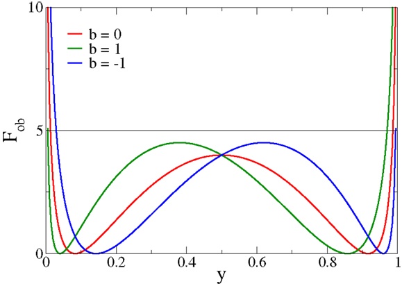
Figure 1. The objective function F_ob, expression (3), as a function of the output firing rate y for different values of the bias b. F_ob always has two minima and diverges for extremal firing rates y → 0/1, a feature responsible for inducing limited output firing rates.

Minimizing Equation (3) as an objective function for deriving synaptic plasticity rules will therefore lead to bounded membrane potentials and hence necessarily to bounded learning rules, devoid of runaway synaptic growth. The cost function [Equation (3)] generically has two distinct minima, a feature setting it apart from other objective functions for synaptic plasticity rules (Intrator and Cooper, 1992). Moreover, the objective function [Equation (3)] can also be motivated by considering the Fisher information of the post-synaptic firing rate with respect to the synaptic flux, as shown in Section 2.1.

In Section 2.2, via stochastic gradient descent, the following plasticity rules for the afferent synaptic weights w_j will be derived:

${ẇ}_j={\mathrm{ϵ}}_{w}G\left(x\right)H\left(x\right)\left(y_j-{ȳ}_j\right),$ (4)

with

$G\left(x\right)=2+x\left(1-2y\right),H\left(x\right)=\left(2y-1\right)+2x\left(1-y\right)y.$ (5)

Here, ϵ_w controls the rate of the synaptic plasticity. The bias b entering the sigmoidal may be either taken to be constant or adapted via

$ḃ=\left(-{\mathrm{ϵ}}_b\right)\left(1-2y+y\left(1-y\right)\mathrm{\lambda }\right),$ (6)

in order to obtain a certain average post-synaptic firing rate, where λ is a control parameter, as detailed out in Section 2.2. Equation (6) leads to the optimization of the statistical information content of the neural activity, in terms of Shannon’s information entropy; a process also denoting intrinsic adaption (Triesch, 2007) or polyhomeostatic optimization (Marković and Gros, 2010).

Both adaption rules, Equation (4) for the synaptic plasticity and Equation (6) for regulating the average post-synaptic firing rate, interfere only weakly. For instance, one could take the bias b as a control parameter, by setting ϵ_b → 0, and measure the resulting mean firing rate a posteriori. The features of the synaptic adaption process remain unaffected and therefore alternative formulations for the intrinsic adaption of the bias could also be considered.

The synaptic plasticity rule [Equation (4)] involves the Hebbian factor H(x), and a multiplicative synaptic weight rescaling factor G(x). Although here G and H are presented as a function of x and y, these can also be expressed entirely in terms of y, consistently with the Hebbian interpretation. It is illustrative to consider the cases of small/large post-synaptic neural activity. In the limit y → 0/1, which is never reached, the updating rules [Equation (4)] would read

${ẇ}_j\propto \left\{\begin{array}{ccc}\hfill \left(2+x\right)\left(-1\right)\left(y_j-{ȳ}_j\right)\hfill & \hfill \hfill & \hfill \left(y\to 0\right)\hfill \\ \hfill \left(2-x\right)\left(+1\right)\left(y_j-{ȳ}_j\right)\hfill & \hfill \hfill & \hfill \left(y\to 1\right)\hfill \\ \hfill \hfill \end{array}\right..$ (7)

For the case that |x| < 2, we hence have that the synaptic strength decreases/increases for an active pre-synaptic neuron with $y_j>{ȳ}_j$, whenever the post-synaptic neuron is inactive/active, an instance of Hebbian learning. The multiplicative constraint (2 ± x) in Equation (7) results in a self-limitation of synaptic growth. Synaptic potentiation is turned into synaptic depression whenever the drive x becomes too large in magnitude. Runaway synaptic growth is hence not possible and the firing rate will settle close to the minima of F_ob, compare Figure 1.

2.1. Motivation in Terms of Fisher Information

The synaptic plasticity rules [Equation (4)] can be derived either directly from the objective function [Equation (3)], as explained in Section 2.2 or motivated from an higher-order principle, the optimization of the synaptic flux, as we will show in the following. Synaptic weight competition could be formulated, as a matter of principles, through an ad hoc constraint like

${\displaystyle \sum _j}{\left(w_j\right)}^2\to \text{const}.,w=\left(w_1,w_2,\dots \right),$ (8)

which defines a hypersphere in the phase of afferent synaptic weights {w_j}, together with some appropriate Hebbian-type adaption rules. We will not make use of Equation (8) explicitly, but our adaption rules implicitly lead to finite length for the synaptic weight vector w.

Synaptic plasticity will modify, quite generically, the statistical properties of the distribution p(y) of the firing rate y of the post-synaptic neuron. It is hence appropriate to consider the sensitivity of the firing-rate distribution p(y) with respect to changes in the w_j. For this purpose, one may make use of the Fisher information

$F_{\mathrm{\theta }}=\int p\left(y\right){\left(\frac{\partial }{\partial \mathrm{\theta }}\ln \left(p\left(y\right)\right)\right)}^{2}dy,$ (9)

which encodes the sensitivity of a given probability distribution function p(y) with respect to a certain parameter θ. Here, we are interested in the sensitivity with respect to changes in the synaptic weights {w_j} and define with

$F_w=\int p\left(y\right){\left({\displaystyle \sum _j}{w}_j\frac{\partial }{\partial w_j}\ln \left(p\left(y\right)\right)\right)}^{2}dy,$ (10)

the Fisher information with respect to the synaptic flux. Expression (10) corresponds to the Fisher information [Equation (9)] when considering

$\frac{\partial }{\partial \mathrm{\theta }}\to {\displaystyle \sum _j}{w}_j\frac{\partial }{\partial w_j}=w\cdot {\nabla }_w,$ (11)

as differential operator. The factors w_j in front of the ∂/∂w_j result in a dimensionless expression, the generating functional [Equation (10)] is then invariant with respect to an overall rescaling of the synaptic weights and the operator Equation (11) a scalar. Alternatively, we observe that $w_j\partial ∕\partial w_j=\partial ∕\partial \log \left(w_j∕w_0\right)$, where w₀ is an arbitrary reference synaptic weight, corresponding to the gradient in the space of logarithmically discounted synaptic weights.

The operator Equation (11), which we denote synaptic flux operator, is, in addition, invariant under rotations within the space of synaptic weights and the performance of the resulting synaptic plasticity rules will hence be also invariant with respect to the orientation of the distributions p(y_j) of the input activities {y_j}. Physically, the operator Equation (11) corresponds, apart from a normalization factor, to the local flux through the synaptic hypersphere, as defined by Equation (8), since the synaptic vector w is parallel to the normal vector through the synaptic hypersphere, as illustrated in Figure 2.

FIGURE 2

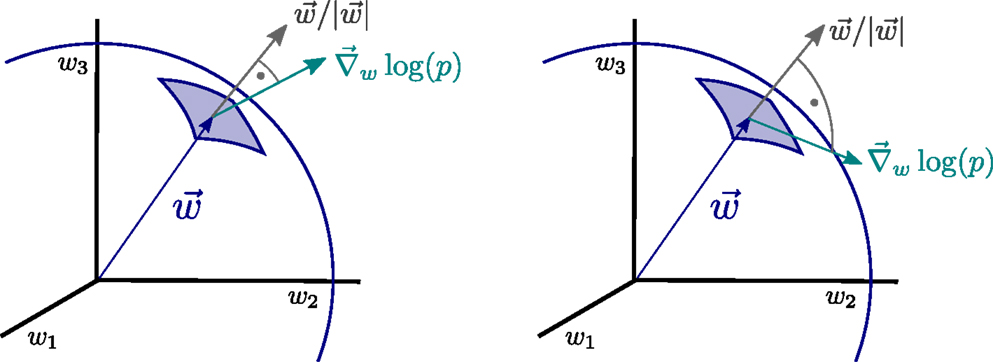
Figure 2. Illustration of the principle of minimal synaptic flux. The synaptic flux, compare expression (11), is the scalar product between the gradient ∇_w log(p) and the normal vector of the synaptic sphere, $\overline{w}∕\left|\overline{w}\right|$ (left). Here, we disregard the normalization. The sensitivity ∇ _w log(p) of the neural firing-rate distribution p = p(y), with respect to the synaptic weights w = (w₁, w₂, w₃, …), vanishes when the local synaptic flux is minimal (right), viz when w ⋅∇ _w log(p) →0. At this point, the magnitude of the synaptic weight vector $\overline{w}$ will not grow anymore.

The Fisher information [Equation (10)] can be considered as a generating functional to be minimized with respect to the synaptic weights {w_j}. The time-averaged properties of the neural activities, as measured by p(y), will then not change any more at optimality; the sensitivity of the neural firing-rate distribution, with respect to the synaptic weights, vanishing for small F_w. At this point, the neuron has finished encoding the information present in the input data stream through appropriate changes of the individual synaptic weights.

It is interesting to consider what would happen if one would maximize the Fisher information instead of minimizing it. Then, the neural firing activity would become very sensitive to small changes in the synaptic weights {w_j} and information processing unstable, being highly susceptible to noise, viz to small statistical fluctuation of the synaptic weights. On a related note, the inverse Fisher information constitutes, via the Cramer–Rao theory (Paradiso, 1988; Seung and Sompolinsky, 1993; Gutnisky and Dragoi, 2008), a lower bound for the variance when estimating an external parameter θ. In this context, the external parameter θ can be estimated more reliably when the Fisher information is larger, viz when the distribution considered is highly sensible to the parameter of interest. This is a different setup. Here, we are not interested in estimating the value of the synaptic weights, but in deducing adaption rules for the {w_j}.

2.2. Synaptic Flux Minimization

We are interested in synaptic plasticity rules which are instantaneous in time, depending only on the actual pre- and post-synaptic firing rates y_j and y. Hence, the actual minimization of the synaptic flux functional [Equation (10)] needs to be valid for arbitrary distributions p(y_j) of the pre-synaptic firing activities {y_j}. The synaptic flux F_w, which is in the first place a functional of the post-synaptic activity p(y), needs therefore to be reformulated in terms of the distributions p(y_j). A faithful representation of the post-synaptic firing-rate distribution entering F_w would involve a convolution over all pre-synaptic p(y_j) and would hence lead to intricate cross-synaptic correlations (Bell and Sejnowski, 1995). Our aim here, however, is to develop synaptic plasticity rules for individual synapses, functionally dependent only on the local pre-synaptic activity and on the overall post-synaptic firing level. We hence consider for the minimization of the synaptic flux all j ∈ {1, …, N_w} synapses separately, viz we replace Equation (10) by

$\begin{array}{llll}\hfill F_w& \to \int {\left({\displaystyle \sum _j}{w}_j\frac{\partial }{\partial w_j}\text{ln}\left(\frac{p\left(y_j\right)}{\mathrm{\partial y}∕\partial y_j}\right)\right)}^2{\displaystyle \prod _l}p\left(y_l\right)d{y}_l& \hfill & \\ \hfill & \equiv \int f_w\left(y\right){\displaystyle \prod _l}p\left(y_l\right)d{y}_l,\end{array}$ (12)

where we have defined the kernel f_w(y). We denote the approximation [Equation (12)] the local synapse approximation, since it involves the substitution of p(y)dy by Π_lp(y_l)dy_l. Expression (12) becomes exact for the case N_w = 1. It corresponds to the case in which the distinct afferent synapses interact only via the overall value of the membrane potential x, as typical for a mean-field approximation. We then find, using the neural model [Equation (1)],

$\frac{\mathrm{\partial y}}{\partial y_j}=y\left(1-y\right)w_j$ (13)

and hence

$\begin{array}{llll}\hfill f_w\left(y\right)& ={\left({\displaystyle \sum _j}{w}_j\left(\frac{1}{w_j}+\left(y_j-{ȳ}_j\right)\left(1-2y\right)\right)\right)}^2& \hfill & \\ \hfill & ={\left(N_w+x\left(1-2y\right)\right)}^2\end{array}$ (14)

where N_w is the number of afferent synapses. The kernel f_w is a function of y only, and not of the individual y_j, since $x={\sum }_j{w}_j\left(y_j-{ȳ}_j\right)$. More fundamentally, this dependency is a consequence of choosing the flux operator [Equation (11)] to be a dimensionless scalar.

Taking N_w → 2 in Equation (14) leads to the objective function [Equation (3)] and results in G(x) and H(x) being proportional to each other’s derivatives, with the roots and maxima, respectively, aligned. We however, also performed simulations using the generic expression (14), with the results changing only weakly and quantitatively.

The synaptic weights are updated so that f_w(y) becomes minimal, ${ẇ}_j\propto -\partial f_w\left(y\right)∕\partial w_j$, obtaining the plasticity rule [Equation (4)]. This procedure corresponds to a stochastic steepest descent of the objective function [Equation (3)], a procedure employed when one is interested in obtaining update rules independent of the actual distributions p(y_j) of the afferent neural activities.

For the derivation, one makes use of $\mathrm{\partial y}∕\partial w_j=\left(y_j-{ȳ}_j\right)\left(1-y\right)y$. The synaptic plasticity rule [Equation (4)] depends via $y_j-{ȳ}_j$ on the activity y_j of the pre-synaptic neuron relatively to its mean firing rate ${ȳ}_j$. This dependence models experimental findings indicating that, in the context of spike timing-dependent plasticity, low-frequency stimulation generically induces causal depression (Lisman and Spruston, 2010; Shouval et al., 2010; Feldman, 2012); one needs above-average firing rates for causal potentiation.

Note that synaptic competition is present implicitly in the updating rule through the membrane potential x, entering both G(x) and H(x), which integrates all individual contributions; the local synapse approximation [Equation (12)] only avoids explicit cross-synaptic learning.

We denote the two factors on the right-hand side of Equation (4), G(x) and H(x), as self-limiting and Hebbian, respectively; with H(x) being, by construction, the derivative of G(x). The derivative of H(x) is also proportional to G(x) since we substituted N_w → 2 in the objective function on the right-hand-side of Equation (14). With this choice, the two factors G(x) and H(x) are hence conjugate to each other.

The synaptic plasticity rule [Equation (4)] works robustly for a wide range of adaption rates ϵ_w, including the case of online learning with constant updating rates. For all simulations presented here, we have used ϵ_w = 0.01. We constrained the activities of the pre-synaptic neurons y_j, for consistency, to the interval [0, 1], which is the same interval of post-synaptic firing rates. Generically, we considered uni- and bi-modal Gaussian inputs centered around ${ȳ}_j=0.5$, with individual standard deviations σ_j. We considered in general σ_j = 0.25 for the direction having the largest variance, the dominant direction, with the other directions having smaller standard deviations, typically by a factor of two.

2.3. Emergent Sliding Threshold

One may invert the sigmoidal σ(x) via x = b − log((1 − y)/y) and express the adaption factors solely in terms of the neural firing rate y. For the Hebbian factor H(x), see Equation (5), one then finds

$H\left(y\right)=\left(2y-1\right)+2y\left(1-y\right)\left[b-\log \left(\left(1-y\right)∕y\right)\right].$ (15)

The bias b hence regulates the crossing point from anti-Hebbian (for low neural activity $y<y_H^{*}$) to Hebbian learning (for large firing rates $y>y_H^{*}$), where $y_H^{*}$ is the root of H(y). $y_H^{*}$ depends only on b (as shown in Figure 3), emerging then indirectly from the formulation of the objective function [Equation (3)], and plays the role of a sliding threshold. This sliding threshold is analogous to the one present in the BCM theory (Bienenstock et al., 1982), which regulates the crossover from anti-Hebbian to Hebbian learning with increasing output activity and which is adapted in order to keep the output activity within a given working regime.

FIGURE 3

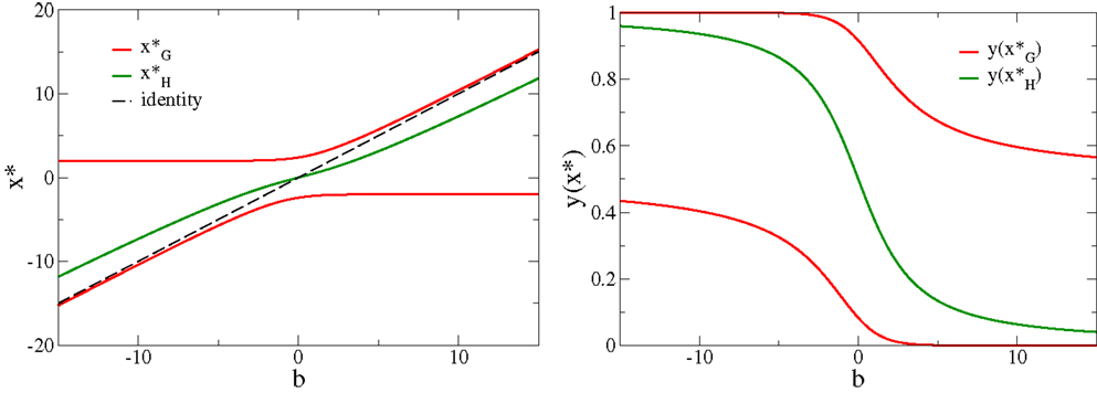
Figure 3. The roots of the adaption factors. Left: the roots $G\left(x_{0,1}^{*}\right)=0$ and H(x*) = 0, respectively, compare Equation (5), as a function of the bias b. Note that the roots do not cross, as the factors G and H are conjugate to each other. Right: the respective values y(x*) of the neural activity. Note that $y\left(x_1^{*}\right)-y\left(x_0^{*}\right)\ge 1∕2$, for all values of the bias.

The bias b regulates, in addition to its role determining the effective sliding threshold for synaptic plasticity, the mean firing rate. In principle, one may consider an ad hoc update rule like $ḃ\propto \left(\mathrm{\mu }-ȳ\right)$ for the bias, where μ = ∫ yp_λ(y)dy is some given target firing rate and where $ȳ$ would be a sliding average of y. We will however use, alternatively, an information theoretical objective function for the intrinsic adaption of the bias. The Kullback–Leibler divergence

$D=\int dyp\left(y\right)\log \left(\frac{p\left(y\right)}{p_{\mathrm{\lambda }}\left(y\right)}\right),p_{\mathrm{\lambda }}\left(y\right)=\frac{{\text{e}}^{\mathrm{\lambda }y}}{N_{\mathrm{\lambda }}}$ (16)

measures the distance between the actual firing-rate distribution p(y) and a given target distribution p_λ(y). It will be minimal if p_λ(y) is approximated as well as possible. An exponential target distribution, as selected here, maximizes the information content of the neural activity in terms of information entropy, given the constraint of a fixed mean μ, both for a finite support y ∈ [0,1], as considered here, as well as for an unbounded support, y > 0, with N_λ being the appropriate normalization factor. For λ → 0, a uniform target distribution is recovered together with μ → 0.5 and the resulting p(y) becomes symmetric with respect to y = 0.5.

Following a derivation which is analogous to the one given above for the case of synaptic flux minimization, one finds Equation (6) for the adaption rules (Triesch, 2007; Linkerhand and Gros, 2013b). For the adaption rate ϵ_b for the bias we used in our simulations generically ϵ_b = 0.1, its actual value having only a marginal influence on the overall behavior of the adaption processes.

Minimizing the Kullback–Leibler divergence and the Fisher information are instances of polyhomeostatic optimization (Marković and Gros, 2010, 2012), as one targets to optimize an entire probability distribution function, here p(y). An update rule like $ḃ\propto \left(\mathrm{\mu }-ȳ\right)$ would, on the other side, correspond to a basic homeostatic control, aiming to regulate a single scalar quantity, such as the mean firing rate.

2.4. Fixpoints of the Limiting Factor

The self-limiting factor G(x) has two roots $x_G^{*}$, compare Figure 3. For b = 0 one finds $x_G^{*}\approx \pm 2.4$ corresponding to firing-rates $y_G^{*}=0.083$ and $y_G^{*}=0.917$, respectively, compare also Figure 3. The roots of G(x) are identical with the two minima of the objective function F_ob, compare the roots of the adaption [Equation (3)]. The self-limiting nature of the synaptic adaption rules [Equation (4)] is a consequence of the two roots of G(x), as larger (in magnitude) membrane potentials will reverse the Hebbian adaption to an anti-Hebbian updating. The roots of G(x) induce, in addition, the tendency of performing a binary classification. As an illustration, consider the case of random sequences of discrete input patterns

$y^{\mathrm{\eta }},\mathrm{\eta }=1,\dots ,N_{patt},$ (17)

with the number of input patterns N_patt being smaller than the number of afferent neurons, N_patt ≤ N_w. The inputs $(y_1,\dots ,y_{N_w})=y$ are selected randomly out of the set [Equation (17)] of N_patt patterns and presented consecutively for small time intervals. The synaptic updating rules will then lead, as we have tested through extended simulations, to a synaptic vector w dividing the space of input patterns into two groups,

$\begin{array}{ccccccc}\hfill w\cdot \left(y^{\mathrm{\eta }}-\overline{\text{y}}\right)\hfill & \hfill =\hfill & \hfill x_G^{*}\left(1\right)\hfill & \hfill \text{for}\hfill & \hfill \mathrm{\gamma }{N}_{patt}\hfill & \hfill \text{states}\hfill & \hfill y^{\mathrm{\eta }}\hfill \\ \hfill w\cdot \left(y^{\mathrm{\eta }}-\overline{\text{y}}\right)\hfill & \hfill =\hfill & \hfill x_G^{*}\left(2\right)\hfill & \hfill \text{for}\hfill & \hfill \left(1-\mathrm{\gamma }\right)N_{patt}\hfill & \hfill \text{states}\hfill & \hfill y^{\mathrm{\eta }}\hfill \\ \hfill \hfill \end{array},$ (18)

which is a solvable set of N_patt equations for N_w variables (w₁, w₂, …). Here, we have denoted with $x_G^{*}\left(1\right)$ and $x_G^{*}\left(2\right)$ the two distinct roots of G(x), and with $\overline{\text{y}}=\left({\sum }_{\mathrm{\eta }}{y}^{\mathrm{\eta }}\right)∕N_{patt}$ the mean input activity. This outcome of the long-term adaption corresponds to a binary classification of the N_patt vectors. The membrane potential x = w⋅y just takes two values, for all inputs y drawn from the set of input patterns.

There is one free parameter in Equation (18), namely the fraction γ and (1 − γ) of patterns mapped to $x_G^{*}\left(1\right)$ and $x_G^{*}\left(2\right)$, respectively. This fraction γ is determined self-consistently by the system, through the polyhomeostatic adaption [Equation (6)] of the bias b, with the system trying to approximate as close as possible the target firing-rate distribution ∝exp(λy), see Equation (16).

3. Results

In order to test the behavior of the neuron under rules [Equation (4, 6)] when presented with different input distributions, a series of numerical simulations have been performed. In the following sections, the evolution of the system when faced with static input distributions is first studied. In particular, principal component extraction and linear discrimination tasks are evaluated. These results are then extended to a scenario of varying input distributions and a fading memory effect is then analyzed.

3.1. Principal Component Extraction

As a first experiment we consider the case of N_w input neurons with Gaussian activity distributions p(y_j). In this setup a single component, namely y₁, has standard deviation σ and all other N_w − 1 directions have a smaller standard deviation of σ/2, as illustrated in Figure 4A. We have selected, for convenience, y₁ as the direction of the principal component. The synaptic updating rule [Equation (1)] is, however, fully rotational invariant in the space of input activities and the results of the simulations are independent of the actual direction of the principal component. We have verified this independence by running simulations with dominant components selected randomly in the space of input activities.

FIGURE 4

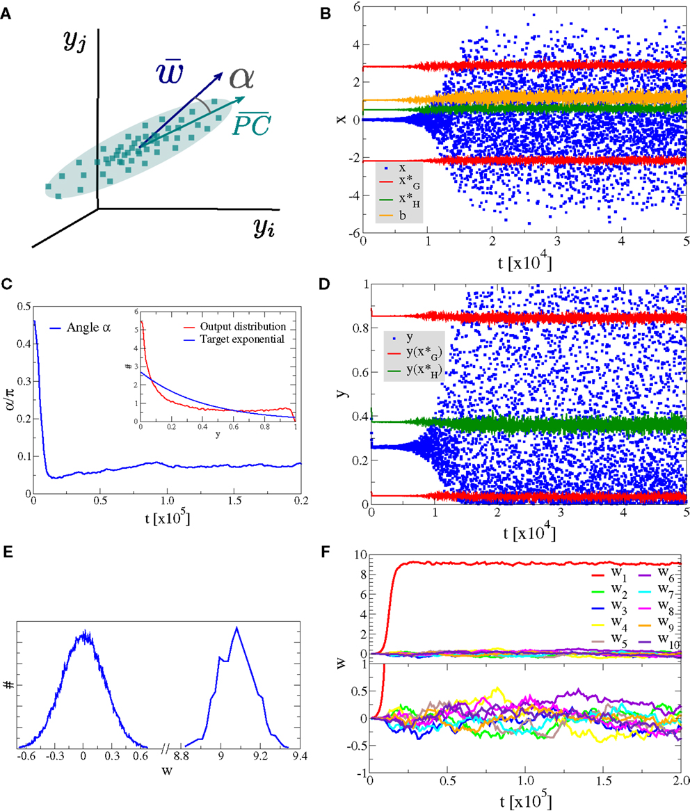
Figure 4. Alignment to the principal component. Simulation results for a neuron with N_w = 100 input neurons with Gaussian input distributions with one direction (the principal component) having twice the standard deviation than the other N_w − 1 directions. (A) Illustration of the input distribution density p(y₁, y₂, …), with the angle α between the direction of the principal component $\left(\overline{PC}\right)$ and $\overline{w}$, the synaptic weight vector. (B) Time series of the membrane potential x (blue), the bias b (yellow), the roots $x_G^{*}$ of the limiting factor G(x) (red), and the root $x_H^{*}$ of the Hebbian factor H(x) (green). (C) The evolution of the angle α of the synaptic weight vector w with respect to the principal component and (inset) the output distribution p(y) (red) with respect to the target exponential (blue). (D) Time series of the output y (blue) and of the roots $y_G^{*}$ of the limiting factor G(y) (red) and the root $y_H^{*}$ of the Hebbian factor H(y) (green). (E) Distribution of synaptic weights p(w) in the stationary state for large times. (F) Time evolution of the first ten synaptic weights {w_j}, separately for the principal component (upper panel) and for nine other orthogonal directions (lower panel).

In Figure 4, we present the result for N_w = 100 afferent neurons and λ = − 2.5 for the target distribution p_λ(y), compare Equation (16) in Section 2. The initial synaptic weights {w_j} have been randomly drawn from [−0.006: 0.005] and are hence quite small, such that the learning rule is initially exclusively Hebbian, viz the membrane potential x is substantially smaller than the roots $x_G^{*}$ of the limiting factor G(x) (compare Figure 4B where $x∕x_G^{*}$ are given by the blue/red dots, respectively). Hebbian synaptic growth then eventually leads to larger weights, with the weight along the principal component (here w₁, red line in Figure 4F) becoming very large. At this stage, the membrane potential x starts to cross the roots $x_G^{*}$ of the limiting factor G(x) and a stationary state results, with the weight along the principal component saturating and with the weights along the non-principal components involved in bounded random drifts. This stationary state, with continuously ongoing online learning, remains stable for arbitrary simulation times.

The firing rate y(t) covers the whole available interval [0, 1], in the stationary state, and a sliding threshold emerges self-consistently. This sliding threshold is given by the root $x_H^{*}$ of the Hebbian factor H(x); learning is Hebbian/anti-Hebbian for $y>y\left(x_H^{*}\right)$ and $y<y\left(x_H^{*}\right)$, respectively. For our simulation, the sliding threshold is about $y\left(x_H^{*}\right)\simeq 0.4$ (green dots in Figure 4D) in the stationary state.

The angle α between the direction of the synaptic weight vector w and the principal component of input activities is initially large, close to the random value of π/2, dropping close to zero with forthgoing synaptic adaption, as shown in Figure 4C, a consequence of the growth of w₁. In Figure 4E, we plot the distribution of the w_j, with a separate scale for the principal component, here w₁ ≈ 9.1 (as averaged over 100 runs). The small components are Gaussian distributed around zero with a standard deviation of ${\mathrm{\sigma }}_w^{\left(non\right)}\approx 0.23$, we have hence a large signal-to-noise ratio of $S_w=\left|w_1\right|∕{\mathrm{\sigma }}_w^{\left(non\right)}\approx 9.1∕0.23\approx 40$.

We also present in the inset of Figure 4C, a comparison between the actual firing-rate distribution p(y) in the stationary state and the exponential target distribution ∝exp(λy), entering the Kullback–Leibler divergence, see Equation (16).

3.2. Signal-to-Noise Scaling

For synaptic adaption rules to be biologically significant they should show stable performance even for large numbers N_w of afferent neurons, without the need for fine-tuning of the parameters. This is the case for our plasticity rules.

In Figure 5, we present the scaling behavior of the synaptic weight configuration. We consider both a large range for the number N_w of afferent neurons and an extended range for the incoming signal-to-noise ratio. The input activity distributions p(y_j) are Gaussians with standard deviations σ_j = σ_⊥for (j = 2, …, N_w), and with the dominant direction having a width σ₁. We define the incoming signal-to-noise ratio as S_i = σ₁/σ_⊥, and investigate values for S_i of 2:1, 4:1, 8:1, 16:1, and 32:1. Shown in Figure 5 is the evolution of the outgoing signal-to-noise ratio, as a function of inputs N_w, and the evolution of the angle α. All simulation parameters are kept otherwise constant.

FIGURE 5

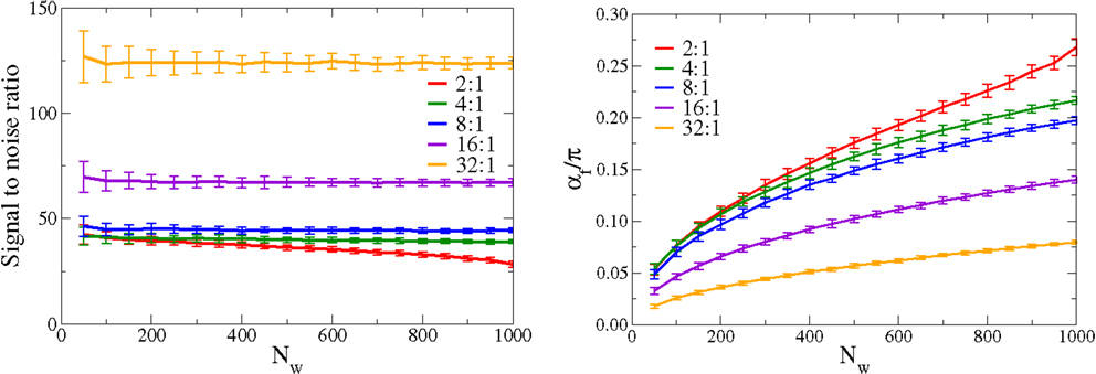
Figure 5. Scaling of the adaption rules with the number of afferent neurons. For constant simulating parameters the signal-to-noise ratio (left), defined as the ratio $\left|w_1\right|∕{\mathrm{\sigma }}_w^{\left(non\right)}$, where w₁ is the synaptic strength parallel to the principal component and ${\mathrm{\sigma }}_w^{\left(non\right)}$ the standard deviation of the orthogonal synaptic directions, compare Equation (A2), and the mean angle (right), of the synaptic weight vector with respect to the principal component. Shown are results for a range, 2:1, 4:1, 8:1, 16:1, and 32:1, of the incoming signal-to-noise ratios, defined as the ratio of the standard deviations between the large and the small components of the distributions of input activities p(y_j). The outgoing signal-to-noise ratio $\left|w_1\right|∕{\mathrm{\sigma }}_w^{\left(non\right)}$ remains essentially flat, as a function of N_w; the increase observed for the average angle α is predominantly a statistical effect, caused by the presence of an increasingly large number of orthogonal synaptic weights. The orthogonal weights are all individually small in magnitude, but their statistical influence sums up increasingly with raising N_w.

We define the outgoing signal-to-noise ratio as $S_w=\left|w_1\right|∕{\mathrm{\sigma }}_w^{\left(non\right)}$ where w₁ is the synaptic weight along the principal component and ${\mathrm{\sigma }}_w^{\left(non\right)}$ the standard deviation of the remaining synaptic weights [compare Equation (A2) in Appendix]. The outgoing signal-to-noise ratio is remarkably independent of the actual number N_w of afferent neurons. S_w shows, in addition, a threshold behavior, remaining finite even for data input streams characterized by small S_i. For large value of incoming signal-to-noise ratio, a linear scaling S_w ∝ S_i is recovered.

Regarding the angle α, the performance deteriorates, which increases steadily with N_w. This is, however, a dominantly statistical effect. In the appendix, we show how the angle α increases with N_w for a constant outgoing signal-to-noise ratio S_w. This effect is then just a property of angles in large dimensional spaces and is independent of the learning rule employed.

It is interesting to compare the simulation results with other updating rules, like Oja’s rule (Oja, 1997),

${ẇ}_j={\mathrm{ϵ}}_{oja}\left[y\left(y_j-{ȳ}_j\right)-\mathrm{\alpha }{y}^2{w}_j\right].$ (19)

The original formulation used α = 1 for the relative weighting of the decay term in Equation (19). We find, however, for the case of non-linear neurons considered here, that Oja’s rule does not converge for α ≳0. 1. For the results presented in Figure 6, we adapted the bias using Equation (6) both when using Oja’s rule [Equation (19)] and for our plasticity rule [Equation (4)]. The parameter ϵ_oja was chosen such that the learning times (or the number of input patterns) needed for convergence matched, in this case ϵ_oja = 0.1. With Oja’s rule, arbitrarily large outgoing signal-to-noise ratios are achievable for α → 0. In this case, the resulting p(y) becomes binary, as expected. There is hence a trade-off and only intermediate values for the outgoing signal-to-noise ratio are achievable for smooth firing-rate distributions p(y). Note that Sanger’s rule (Sanger, 1989) reduces to Oja’s rule for the case of a single neuron, as considered here.

FIGURE 6

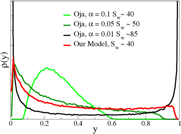
Figure 6. The output distribution function and the signal-to-noise ratio. The averaged firing-rate distributions p(y) for N_w = 100 and the parameter set used previously, compare Figure 5. In comparison, the p(y) resulted when using a modified Oja’s rule, see Equation (19), for the synaptic plasticity. Depending on the parameter ϵ, controlling the strength of the weight decay in Equation (19), arbitrary large signal-to-noise ratios S_w can be achieved, on the expense of obtaining binary output distributions. Note that the form of p(y) is roughly comparable, for similar signal-to-noise ratios, for the two approaches. The output tends to cluster, however, around the target mean for smaller S_w and Oja’s rule.

We also attempted to compare with the results of the BCM theory (Bienenstock et al., 1982; Intrator and Cooper, 1992; Cooper and Bear, 2012). The BCM update rule also finds nicely the direction of the principal component, but runaway synaptic growth occurs generically in the case of the type of neurons considered in our study, being non-linear and having an maximal possible firing rate, with y ∈ [0, 1]. This is due to the fact that the upper cut-off of the firing rate preempts, in general, the sliding threshold to raise to values necessary to induce a large enough amount of synaptic weight decay. For the input distributions used throughout this study, we could not avoid runaway synaptic growth for the BCM rule.

3.3. Linear Discrimination

An important question regards the behavior of neural learning rules when no distinct principal component is present in the data input stream. In Figure 7, we present data for the situation where two dominant directions have the same standard deviation σ ≈ 0.22, here for p(y₁) and p(y₂), with the remaining N_w − 2 directions having a smaller standard deviation σ/4. In our experiment the first direction, y₁ is a unimodal Gaussian, as illustrated in Figure 7A, with the second direction, y₂ being bimodal. The two superposed Gaussian distributions along y₂ have individual widths σ/4 and the distance between the two maxima has been adjusted so that the overall standard deviation along y₂ is also σ.

FIGURE 7

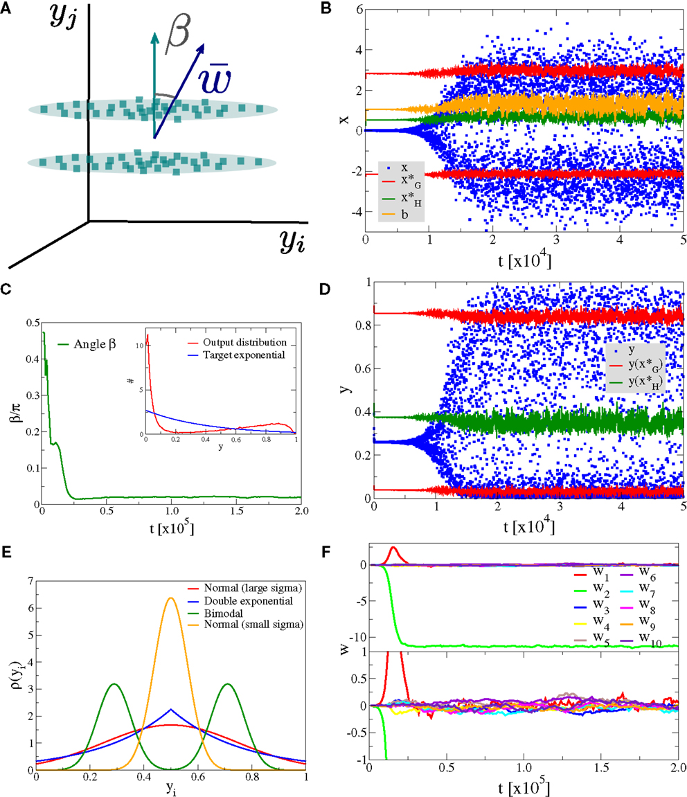
Figure 7. Linear discrimination of bimodal input distributions. Simulation results for a neuron with N_w = 100 with two directions having the same variance (but one being bimodal) and the other N_w − 2 directions having a standard deviation four times smaller. (A) Illustration of the input distribution density p(y₁, y₂, …). (B) Time series of the membrane potential x (blue), the bias b (yellow), the roots $x_G^{*}$ of the limiting factor G(x) (red), and the root $x_H^{*}$ of the Hebbian factor H(x) (green). (C) The evolution of the angle β of the synaptic weight vector w with respect to the axis linking the two ellipsoids and (inset) the output distribution p(y) (red) in comparison to the target exponential (blue). (D) Time series of the output y (blue) and of the roots $y_G^{*}$ of the limiting factor G(y) (red) and the root $y_H^{*}$ of the Hebbian factor H(y) (green). (E) Illustration of the distribution functions used, the bimodal competing with the Normal distributed (alternatively with a double exponential) having the same variance, all other directions being normally distributed with a four times smaller standard distribution. (F) Time evolution of the first ten synaptic weights {w_j}, separately for the principal component (upper panel) and for nine other orthogonal directions (lower panel).

The synaptic weight vector aligns, for most randomly drawn starting ensembles {w_j}, with the bimodal direction, as shown in Figures 7C,F. In this case the system tries to adjust its parameters, namely the synaptic weights and the bias b so that the two peaks of the bimodal principal component are close to the two zeros $x_G^{*}$ (red symbols in Figure 7B) of the limiting factor G(x) in the adaption rule [Equation (4)]. This effect is clearly present in the results for the membrane potential (blue symbols in Figure 7B), clustering around the roots of G(x). The system performs, as a result, a linear discrimination with a bimodal output firing rate, presented in Figure 7D.

One possibility to characterize the deviation of a probability distribution from a Gaussian is the excess kurtosis κ (DeCarlo, 1997),

$\begin{array}{llll}\hfill & \mathrm{\kappa }=\frac{Q_j}{{\mathrm{\sigma }}_j^4}-3,Q_j=\int {\left(y_j-{ȳ}_j\right)}^{4}p\left(y_j\right)d{y}_j,& \hfill & \\ \hfill & {\mathrm{\sigma }}_j^2=\int {\left(y_j-{ȳ}_j\right)}^{2}p\left(y_j\right)d{y}_j,\end{array}$ (20)

with the normal distribution having, by construction, a vanishing κ → 0. The excess kurtosis tends to be small or negative on a finite support p_j ∈ [0, 1]. Distributions characterized by a positive κ show pronounced tails. This statement also holds for truncated Gaussians, as used in our simulations. We have generalized the experiment presented in Figure 7 by studying the pairwise competition between three distributions having all the same standard deviation σ, but varying values of κ, compare Figure 7E: a bimodal distribution with κ = − 1.69, a unimodal Gaussian with κ = − 0.63, and a unimodal double exponential with κ = − 0.43.

Running the simulation one thousand times, with randomly drawn initial conditions, the direction with lower κ was selected 88.8/65.4/64.0% of the times when the competing directions were bimodal vs. double exponential/Gaussian vs. double exponential/bimodal vs. Gaussian. In none of the cases would both the first and the second synaptic weights, w₁ and w₂, acquire large absolute values.

The underlying rationale for the updating rules favoring directions with negative excess kurtosis can be traced back to the inherent symmetry F_ob(−x, 1 − y) = F_ob(x, y) of the objective function [Equation (3)], which in turn is a consequence of treating both large and small firing rates on an equal footing in F_ob. There are two equivalent minima for F_ob to which the maxima of a binary distribution are mapped, as discussed in Section 2.

We have repeated this simulation using the modified Oja’s rule [Equation (19)], using α = 0.1 and ϵ_oja = 0.1. We find a very distinct sensitivity, with the relative probability for a certain input direction to be selected being 97.0/99.8/42.1% when the competing directions were bimodal vs. double exponential/Gaussian vs. double exponential/bimodal vs. Gaussian. Note that all our input distributions are centered around 0.5 and truncated to [0, 1]. Oja’s rule has a preference for unimodal distributions and a strong dislike of double exponentials. However, the excess kurtosis does not seem to be a determining parameter, within Oja’s rule, for the directional selectivity.

3.4. Continuous Online Learning–Fading Memory

Another aspect of relevance concerns the behavior of synaptic plasticity rules for continuous online learning. A basic requirement is the absence of runaway growth effects in the presence of stationary input statistics. But how should a neuron react when the statistics of the afferent input stream changes at a certain point? Should it adapt immediately, at a very short time scale or should it show a certain resilience, adapting to the new stimuli only when these show a certain persistence?

We have examined the behavior of the adaption rules upon a sudden change of firing-rate statistics of the afferent neurons. We find, as presented in Figure 8, that the new statistics is recognized autonomously, with a considerable resilience to unlearn the previously acquired information about the statistics of the input data stream. The synaptic plasticity rules [Equation (4)] do hence incorporate a fading memory.

FIGURE 8

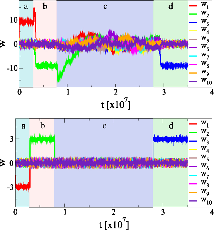
Figure 8. Continuous online learning and weak forgetting. The effect of changing the statistics of the input firing rates p(y_j). During (a), (b), and (d) the principal axis is along y₁, y₂, and y₃, respectively, during (c) there in no principal component. There are N_w = 100 afferent neurons, shown is the time evolution of the first ten synaptic weights. The standard deviations of the afferent neurons is σ for the principal direction, if there is any, and σ/2 for all other directions, compare Figure 4. During(c), all inputs have identical standard deviations σ/2. The initial weight distribution is randomly drawn. The top/bottom panel shows the results using, respectively, our synaptic updating rule [Equation (4)] and Oja’s rule [Equation (19)]. Note that it takes considerably longer, for our updating rule, to unlearn than to learn from scratch. Learning and unlearning occurs, on the other side, at the same timescale for Oja’s rule.

In our experiment, we considered N_w = 100 afferent neurons, with Gaussian firing distributions having standard deviation σ for the principal component and σ/2 for the remaining N_w − 1 directions. The sign of the synaptic weights are not of relevance, as the input distributions p(y_j) are symmetric with respect to their means, taken to be 0.5. The direction of the principal component is then changed several times, everything else remaining otherwise unchanged.

The starting configuration {w_j} of synaptic weights has been drawn randomly from [−0.005: 0005] and the initial learning is fast, occurring on a time scale of T_initial ≈ 10⁴ updatings, compare Figure 4, using the same updating rates ϵ_w = 0.01 and ϵ_b = 0.1 throughout this paper. The time the neuron takes to adapt to the new input statistics is, however, of the order of T_unlearn ≈ 10⁶, viz about two orders of magnitude larger than T_initial. New information is hence acquired at a slower rate; the system shows a substantial resilience to unlearn previously acquired memories.

One can observe in Figure 8 an overshoot of the principal synaptic weight, just before the unlearning starts, as the system tries to keep the membrane potential x within its working regime, compare Figure 4D. The system reacts by increasing the largest synaptic weight when the variance of the input drops along the corresponding afferent direction, before it can notice that the principal component of the afferent activities has also changed.

Also included in the simulation presented in Figure 8 is a phase without any principal component, the statistics of all incoming p(y_j) being identical, viz with the covariance matrix being proportional to unity. One notices that the neuron shows a marked resilience to forget the previously acquired knowledge, taking about 5 × 10⁷ updates in order to return to a fully randomized drifting configuration of synaptic weights {w_j}. The synaptic plasticity rule [Equation (4)] hence leads to an extended fading memory, which we believe to be a consequence of its multiplicative structure.

For comparison we have repeated the same experiment using the modified Oja’s rule [Equation (19)], using α = 0.1 (which yields the same signal-to-noise ratio, compare Figure 6), and ϵ_oja = 0.1, such that the initial learning rates (achieving 90% of the stationary value for the principal component) are comparable for both updating rules. We also kept the same updating Equation (6) for the bias. For Oja’s rule learning and unlearning occurs on very similar time scales, reacting immediately to changes in the statistics of the input activities.

It is presently not entirely clear which form of unlearning is present in the brain, on the level of individual neurons. While studies in prefrontal cortex have shown full learning and unlearning of different categories in binary classification tasks, related in this context to the concept of adaptive coding (Duncan, 2001), more complex behavioral responses tend, however, to exhibit slow or incomplete unlearning such as extinction of paired cue–response associations, in the context of Pavlovian conditioning (Myers and Davis, 2002; Quirk and Mueller, 2007). It is also conceivable that a fading memory may possibly be advantageous in the context of noisy environments with fluctuating activity statistics.

4. Discussion

Objective functions based on information theoretical principles play an important role in neuroscience (Intrator and Cooper, 1992; Lengellé and Denoeux, 1996; Goodhill and Sejnowski, 1997; Kay and Phillips, 2011) and cognitive robotics (Sporns and Lungarella, 2006; Ay et al., 2008). Many objective functions investigated hitherto use either Shannon’s information directly, or indirectly by considering related measures, like predictive and mutual entropy (Kraskov et al., 2004), or the Kullback–Leibler divergence. Objective functions are instances, from a somewhat larger perspective, of generating functionals, as they are normally used to derive equations of motion for the neural activity, or to deduce adaption rules for secondary variables like synaptic weights or intrinsic parameters. Here, we discuss an objective function which may be either motivated by its own virtue, as discussed in Section 2, or by considering the Fisher information as a generating functional.

The Fisher information encodes the sensitivity of a given probability distribution function, in our case the distribution of neural firing rates, with respect to a certain parameter of interest. Cognitive information processing in the brain is all about changing the neural firing statistics and we hence believe that the Fisher information constitutes an interesting starting point from where to formulate guiding principles for plasticity in the brain or in artificial systems. In particular, we have examined the Fisher information with respect to changes of the synaptic weights. Minimizing this objective function, which we denoted as the synaptic flux, we find self-limiting adaption rules for unsupervised and autonomous learning. The adaption rules are Hebbian, with the self-limitation leading to synaptic competition and an alignment of the synaptic weight vector with the principal component of the input data stream.

Synaptic plasticity rules for rate encoding neurons are crucial for artificial neural networks used for cognitive tasks and machine learning, and important for the interpretation of the time-averaged behavior of spiking neurons. In this context our adaption rules make two predictions, which one may eventually test experimentally. The first prediction concerns the adaption in the situation where more than one dominant component is present in the space of input activities. Our model implies for this case a robust tendency for the synaptic weight vector to favor directions in the space of input activities being bimodal, characterized by a negative kurtosis.

Our adaption rules have a second implication, regarding the robustness of acquired memories with respect to persistent changes of the statistics of the input activities, in the context of continuous and unsupervised online learning. We predict that it is considerably easier for the neuron to detect relevant features in the space of input activities when starting from a virgin state of a random synaptic configuration. New features will still be extracted from the stream of input activities, and old ones unlearned at the same time, once the initial synaptic adaption process has been completed, albeit at a much slower pace. This feature can be interpreted as a sturdy fading memory.

We have extensively examined the robustness of the behavior of the synaptic plasticity rules upon variation of the simulation setup. All results presented here remain fully valid when changing, e.g., the adaption rate ϵ_w, in particular we have examined ϵ_w = 0.1 and ϵ_w = 0.001. We have also studied other forms of input activities p(y_j) and found only quantitative changes for the response. For example, we have considered exponentially distributed input statistics, as a consistency check with the target output distribution function. We hence believe that the here proposed synaptic plasticity rules are robust to a considerable degree, a prerequisite for viable plasticity rules, both in the context of biological and artificial systems.

The synaptic plasticity rule [Equation (4)] is a product of two conjugate factors, the limiting factor G(x) and the Hebbian factor H(x). Runaway synaptic growth occurs, as we have verified numerically, when setting G(x) to a constant. Unlimited synaptic growth occurs despite the emergence of a sliding threshold [see Equation (15) of Section 2] as the firing rate y(t) ∈ [0,1] is bounded. Runaway synaptic growth results in increasing (positive and negative) large membrane potentials x(t), with the firing becoming binary, accumulating at the boundaries, viz y → 0 and y → 1.

Finally, we comment on the conceptual foundations of this work. The adaptive time evolution of neural networks and the continuous reconfiguration of synaptic weights may be viewed as a self-organizing processes guided by certain target objectives (Prokopenko, 2009; Friston, 2010; Gros, 2010; Linkerhand and Gros, 2013a). A single objective function will in general not be enough for generating dynamics of sufficient complexity, as necessary for neural circuitry or synaptic reconfiguration processes. It has indeed been noted that the interplay between two or more generating functionals may give rise to highly non-trivial dynamical states (Linkerhand and Gros, 2013a; Gros, 2014).

In this context, it is important to note that several generating functionals may in general not be combined to a single overarching objective function. Dynamical systems can hence show, under the influence of competing objective functions, complex self-organizing behavior (Linkerhand and Gros, 2013a; Gros, 2014). In the present work, we propose that the interplay between two specific objective functions, namely the Fisher information for the synaptic flux and the Kullback–Leibler divergence for the information content of the neural firing rate, give rise, quite naturally, to a set of viable adaption rules for self-limiting synaptic and intrinsic plasticity rules.

Conflict of Interest Statement

The authors declare that the research was conducted in the absence of any commercial or financial relationships that could be construed as a potential conflict of interest.

Acknowledgments

Rodrigo Echeveste acknowledges stimulating discussions at the OCCAM 2013 workshop. The support of the German Science Foundation (DFG) is acknowledged.

References

Abbott, L. F., and Nelson, S. B. (2000). Synaptic plasticity: taming the beast. Nat. Neurosci. 3, 1178–1183. doi: 10.1038/78829

Pubmed Abstract | Pubmed Full Text | CrossRef Full Text

Ay, N., Bertschinger, N., Der, R., Güttler, F., and Olbrich, E. (2008). Predictive information and explorative behavior of autonomous robots. Eur. Phys. J. B 63, 329–339. doi:10.1140/epjb/e2008-00175-0

CrossRef Full Text

Bell, A. J., and Sejnowski, T. J. (1995). An information-maximization approach to blind separation and blind deconvolution. Neural Comput. 7, 1129–1159. doi:10.1162/neco.1995.7.6.1129

Pubmed Abstract | Pubmed Full Text | CrossRef Full Text

Bienenstock, E. L., Cooper, L. N., and Munro, P. W. (1982). Theory for the development of neuron selectivity: orientation specificity and binocular interaction in visual cortex. J. Neurosci. 2, 32–48.

Pubmed Abstract | Pubmed Full Text

Brunel, N., and Nadal, J.-P. (1998). Mutual information, Fisher information, and population coding. Neural Comput. 10, 1731–1757. doi:10.1162/089976698300017115

Pubmed Abstract | Pubmed Full Text | CrossRef Full Text

Chagnac-Amitai, Y., Luhmann, H. J., and Prince, D. A. (1990). Burst generating and regular spiking layer 5 pyramidal neurons of rat neocortex have different morphological features. J. Comp. Neurol. 296, 598–613. doi:10.1002/cne.902960407

Pubmed Abstract | Pubmed Full Text | CrossRef Full Text

Cooper, L. N., and Bear, M. F. (2012). The BCM theory of synapse modification at 30: interaction of theory with experiment. Nat. Rev. Neurosci. 13, 798–810. doi:10.1038/nrn3353

Pubmed Abstract | Pubmed Full Text | CrossRef Full Text

DeCarlo, L. T. (1997). On the meaning and use of kurtosis. Psychol. Methods 2, 292–307. doi:10.1037/1082-989X.2.3.292

CrossRef Full Text

DiCarlo, J. J., Zoccolan, D., and Rust, N. C. (2012). How does the brain solve visual object recognition? Neuron 73, 415–434. doi:10.1016/j.neuron.2012.01.010

Pubmed Abstract | Pubmed Full Text | CrossRef Full Text

Dong, D. W., and Hopfield, J. J. (1992). Dynamic properties of neural networks with adapting synapses. Netw. Comput. Neural Syst. 3, 267–283. doi:10.1088/0954-898X/3/3/002

CrossRef Full Text

Duncan, J. (2001). An adaptive coding model of neural function in prefrontal cortex. Nat. Rev. Neurosci. 2, 820–829. doi:10.1038/35097575

CrossRef Full Text

Elliott, T. (2003). An analysis of synaptic normalization in a general class of Hebbian models. Neural Comput. 15, 937–963. doi:10.1162/08997660360581967

Pubmed Abstract | Pubmed Full Text | CrossRef Full Text

Feldman, D. E. (2012). The spike-timing dependence of plasticity. Neuron 75, 556–571. doi:10.1016/j.neuron.2012.08.001

Pubmed Abstract | Pubmed Full Text | CrossRef Full Text

Friston, K. (2010). The free-energy principle: a unified brain theory? Nat. Rev. Neurosci. 11, 127–138. doi:10.1038/nrn2787

Pubmed Abstract | Pubmed Full Text | CrossRef Full Text

Goodhill, G. J., and Barrow, H. G. (1994). The role of weight normalization in competitive learning. Neural Comput. 6, 255–269. doi:10.1162/neco.1994.6.2.255

CrossRef Full Text

Goodhill, G. J., and Sejnowski, T. J. (1997). A unifying objective function for topographic mappings. Neural Comput. 9, 1291–1303. doi:10.1162/neco.1997.9.6.1291

CrossRef Full Text

Gros, C. (2010). Complex and Adaptive Dynamical Systems: A Primer. Heidelberg: Springer-Verlag.

Gros, C. (2014). “Generating functionals for guided self-organization,” in Guided Self-Organization: Inception, ed. M. Prokopenko (Heidelberg: Springer), 53–66.

Gutnisky, D. A., and Dragoi, V. (2008). Adaptive coding of visual information in neural populations. Nature 452, 220–224. doi:10.1038/nature06563

CrossRef Full Text

Hebb, D. O. (2002). The Organization of Behavior: A Neuropsychological Theory. Routledge: Psychology Press.

Huber, P. J. (1985). Projection pursuit. Ann. Stat. 13, 435–475. doi:10.1214/aos/1176349519

CrossRef Full Text

Intrator, N., and Cooper, L. N. (1992). Objective function formulation of the BCM theory of visual cortical plasticity: statistical connections, stability conditions. Neural Netw. 5, 3–17. doi:10.1016/S0893-6080(05)80003-6

CrossRef Full Text

Jain, A. K., Duin, R. P. W., and Mao, J. (2000). Statistical pattern recognition: a review. IEEE Trans. 22, 4–37. doi:10.1109/34.824819

CrossRef Full Text

Kay, J. W., and Phillips, W. (2011). Coherent infomax as a computational goal for neural systems. Bull. Math. Biol. 73, 344–372. doi:10.1007/s11538-010-9564-x

Pubmed Abstract | Pubmed Full Text | CrossRef Full Text

Kraskov, A., Stögbauer, H., and Grassberger, P. (2004). Estimating mutual information. Phys. Rev E 69, 066138. doi:10.1103/PhysRevE.69.066138

Pubmed Abstract | Pubmed Full Text | CrossRef Full Text

Lengellé, R., and Denoeux, T. (1996). Training MLPS layer by layer using an objective function for internal representations. Neural Netw. 9, 83–97. doi:10.1016/0893-6080(95)00096-8

CrossRef Full Text

Linkerhand, M., and Gros, C. (2013a). Generating functionals for autonomous latching dynamics in attractor relict networks. Sci. Rep. 3:2042. doi:10.1038/srep02042

Pubmed Abstract | Pubmed Full Text | CrossRef Full Text

Linkerhand, M., and Gros, C. (2013b). Self-organized stochastic tipping in slow-fast dynamical systems. Math. Mech. Complex Sys. 1-2, 129. doi:10.2140/memocs.2013.1.129

CrossRef Full Text

Lisman, J., and Spruston, N. (2010). Questions about STDP as a general model of synaptic plasticity. Front. Synaptic Neurosci. 2, doi:10.3389/fnsyn.2010.00140

Pubmed Abstract | Pubmed Full Text | CrossRef Full Text

Lisman, J. E. (1997). Bursts as a unit of neural information: making unreliable synapses reliable. Trends Neurosci. 20, 38–43. doi:10.1016/S0166-2236(96)10070-9

Pubmed Abstract | Pubmed Full Text | CrossRef Full Text

Marković, D., and Gros, C. (2010). Self-organized chaos through polyhomeostatic optimization. Phys. Rev. Lett. 105, 068702. doi:10.1103/PhysRevLett.105.068702

Pubmed Abstract | Pubmed Full Text | CrossRef Full Text

Marković, D., and Gros, C. (2012). Intrinsic adaptation in autonomous recurrent neural networks. Neural Comput. 24, 523–540. doi:10.1162/NECO_a_00232

Pubmed Abstract | Pubmed Full Text | CrossRef Full Text

Miller, K. D., and MacKay, D. J. (1994). The role of constraints in Hebbian learning. Neural Comput. 6, 100–126. doi:10.1162/neco.1994.6.1.100

CrossRef Full Text

Myers, K. M., and Davis, M. (2002). Behavioral and neural analysis of extinction. Neuron 36, 567–584. doi:10.1016/S0896-6273(02)01064-4

CrossRef Full Text

Nagy, A. (2003). Fisher information in density functional theory. J. Chem. Phys. 119, 9401–9405. doi:10.1063/1.1615765

Pubmed Abstract | Pubmed Full Text | CrossRef Full Text

Oja, E. (1992). Principal components, minor components, and linear neural networks. Neural Netw. 5, 927–935. doi:10.1016/S0893-6080(05)80089-9

Pubmed Abstract | Pubmed Full Text | CrossRef Full Text

Oja, E. (1997). The nonlinear PCA learning rule in independent component analysis. Neurocomputing 17, 25–45. doi:10.1016/S0925-2312(97)00045-3

Pubmed Abstract | Pubmed Full Text | CrossRef Full Text

Paradiso, M. (1988). A theory for the use of visual orientation information which exploits the columnar structure of striate cortex. Biol. Cybern. 58, 35–49. doi:10.1007/BF00363954

Pubmed Abstract | Pubmed Full Text | CrossRef Full Text

Prokopenko, M. (2009). Guided self-organization. HFSP J. 3, 287–289. doi:10.2976/1.3233933

CrossRef Full Text

Prokopenko, M., Lizier, J. T., Obst, O., and Wang, X. R. (2011). Relating Fisher information to order parameters. Phys. Rev. E 84, 041116. doi:10.1103/PhysRevE.84.041116

Pubmed Abstract | Pubmed Full Text | CrossRef Full Text

Quirk, G. J., and Mueller, D. (2007). Neural mechanisms of extinction learning and retrieval. Neuropsychopharmacology 33, 56–72. doi:10.1038/sj.npp.1301555

CrossRef Full Text

Reginatto, M. (1998). Derivation of the equations of nonrelativistic quantum mechanics using the principle of minimum Fisher information. Phys. Rev. A 58, 1775–1778. doi:10.1103/PhysRevA.58.1775

CrossRef Full Text

Sanger, T. D. (1989). Optimal unsupervised learning in a single-layer linear feedforward neural network. Neural Netw. 2, 459–473. doi:10.1016/0893-6080(89)90044-0

CrossRef Full Text

Seung, H., and Sompolinsky, H. (1993). Simple models for reading neuronal population codes. Proc. Natl. Acad. Sci. U.S.A. 90, 10749–10753. doi:10.1073/pnas.90.22.10749

Pubmed Abstract | Pubmed Full Text | CrossRef Full Text

Shouval, H. Z., Wang, S. S.-H., and Wittenberg, G. M. (2010). Spike timing dependent plasticity: a consequence of more fundamental learning rules. Front. Comput. Neurosci. 4, doi:10.3389/fncom.2010.00019

Pubmed Abstract | Pubmed Full Text | CrossRef Full Text

Simoncelli, E. P., and Olshausen, B. A. (2001). Natural image statistics and neural representation. Annu. Rev. Neurosci. 24, 1193–1216. doi:10.1146/annurev.neuro.24.1.1193

Pubmed Abstract | Pubmed Full Text | CrossRef Full Text

Sinz, F., and Bethge, M. (2013). Temporal adaptation enhances efficient contrast gain control on natural images. PLoS Comput. Biol. 9:e1002889. doi:10.1371/journal.pcbi.1002889

Pubmed Abstract | Pubmed Full Text | CrossRef Full Text

Sporns, O., and Lungarella, M. (2006). “Evolving coordinated behavior by maximizing information structure,” in Artificial Life X: Proceedings of the Tenth International Conference on the Simulation and Synthesis of Living Systems (Cambridge, MA: MIT Press), 323–329.

Triesch, J. (2007). Synergies between intrinsic and synaptic plasticity mechanisms. Neural Comput. 19, 885–909. doi:10.1162/neco.2007.19.4.885

Pubmed Abstract | Pubmed Full Text | CrossRef Full Text

Turrigiano, G. G., and Nelson, S. B. (2000). Hebb and homeostasis in neuronal plasticity. Curr. Opin. Neurobiol. 10, 358–364. doi:10.1016/S0959-4388(00)00091-X

CrossRef Full Text

Vicente, R., Wibral, M., Lindner, M., and Pipa, G. (2011). Transfer entropy: a model-free measure of effective connectivity for the neurosciences. J. Comput. Neurosci. 30, 45–67. doi:10.1007/s10827-010-0262-3

Pubmed Abstract | Pubmed Full Text | CrossRef Full Text

Wiskott, L., and Sejnowski, T. J. (2002). Slow feature analysis: unsupervised learning of invariances. Neural Comput. 14, 715–770. doi:10.1162/089976602317318938

Pubmed Abstract | Pubmed Full Text | CrossRef Full Text

Appendix

Modeling Adaption for Large Numbers of Transversal Directions

For simulations with N_w Gaussian input distributions p(y_j), the synaptic weight vector adapts to

$w=\left(w_1,w_2,\dots ,w_{N_w}\right),w_1\gg w_k\left(k\ge 2\right),$ (A1)

when p(y₁) is assumed to have the largest standard deviation σ₁, with all other p(y_k), for k = 2, …, N_w having a smaller standard deviation σ_k. The angle α between the synaptic weight vector and the direction (1, 0, …, 0) of the principal component is hence given by

$\begin{array}{llll}\hfill \cos \left(\mathrm{\alpha }\right)& =\frac{w_1}{\sqrt{w_1^2+{\sum }_{k>1}{w}_k^2}}=\frac{w_1}{\sqrt{w_1^2+\left(N_w-1\right){\left({\mathrm{\sigma }}_w^{\left(non\right)}\right)}^2}}& \hfill & \\ \hfill & \approx \frac{1}{\sqrt{N_w}}\frac{w_1}{{\mathrm{\sigma }}_w^{\left(non\right)}},\end{array}$ (A2)

where we have defined with ${\mathrm{\sigma }}_w^{\left(non\right)}=\left({\sum }_{k>1}{w}_k^2\right)∕\left(N_w-1\right)$ the averaged standard deviation of the non-principal components (which have generically a vanishing mean). In our simulation we find, compare Figure 5, an outgoing signal-to-noise ratio $S_w=\left|w_1\right|∕{\mathrm{\sigma }}_w^{\left(non\right)}$ which is remarkably independent of N_w and hence that α approaches π/2 like $\pi /2-r/\sqrt{N_w}$ in the limit of large numbers N_w → ∞ of afferent neurons, where r is a constant, independent of N_w. This statistical degradation of the performance, in terms of the angle α, is hence a variant of the well-known curse of dimensionality (Jain et al., 2000).