Event-triggered decision propagation in proximity networks

1. Introduction

Application of mobile sensor networks for monitoring environment is increasingly ubiquitous for both military applications such as undersea mine hunting, anti-submarine warfare, and non-military applications such as weather monitoring and prediction (Lehning et al., 2009; Choi and How, 2011; Mukherjee et al., 2011). This is primarily due to the potential advantages in terms of coverage and time-criticality over their static counterparts. In many applications, the regions of surveillance are remote with limited or unreliable long-range communication and GPS capabilities. Further, accurate sensing becomes a difficult proposition due to environmental disturbances. Therefore, techniques for information management (e.g., decision propagation, trust establishment, positioning, and localization (Baras and Jiang, 2005; Yildiz et al., 2010, 2011)) are often employed using only limited communication. The agents typically receive disparate information from the environment and process it locally in the context of the information obtained from the spatial neighbors. A particular case where all the agents are expected to arrive at a consensus is described in Molavi et al. (2013).

In a recent work Sarkar et al. (2013), the present authors proposed a generalized gossip algorithm in the context of proximity networks to address the issue of distributed decision propagation in a mobile ad hoc sensor network. The study presented interaction between the physical and cyber aspects of the problem, namely, (i) network topology evolution due to agent mobility and (ii) information spreading dynamics, respectively. Results show that the (user-defined) generalizing parameter in the agent interaction policy can control the trade-off between Propagation Radius (i.e., how far a decision spreads from its source) and Localization Gradient (i.e., the extent to which the spatial variations may affect localization of the source), as well as the temporal convergence properties. Although this policy efficiently facilitates distributed decision propagation in a mobile-agent network, this is particularly not efficient in terms of energy consumption by the agents. This is due to the fact that, in the applications discussed above, the events of interest are typically rare and random (Srivastav et al., 2009). Moreover, the agents are preferred to have long life-cycles as re-deployment of such agents is typically very expensive (Salhieh and Schwiebert, 2004). The energy consuming tasks for an agent in the present context include sensing, mobility, and communication (message transmission and reception). For a sparse agent population in a relatively large area of surveillance, task load of sensing and mobility may not be reduced. However, if the communication is considered as an event-triggered task Wan and Lemmon (2009) as opposed to a persistent one, the agents potentially can save significant amount of energy given that events of interest are rare and random. A distributed event-triggered strategy for communication has been shown to reduce the number of messages transmitted over sensor networks (Tabuada, 2007; Mazo and Tabuada, 2008). The key idea of the present work is an extension of the generalized gossip policy to make it more energy efficient by reducing the number of messages transmitted while meeting certain performance criteria.

The idea is implemented by using a simple feedback policy where an agent’s communication activity gets determined by its belief regarding the occurrence of an event of interest in the region of surveillance. However, under this policy the network system can be susceptible to false alarms raised by the sensors (agents). The study therefore introduces a notion of false alarm to investigate its impact on energy saving. The specific contributions of this paper beyond the existing work by the authors are

1. An event-triggered formulation of generalized gossip policy to save energy and increase agents’ lives;

2. Analytical results and simulation-based validation regarding impacts of event-triggered policy on decision propagation characteristics;

3. Analytical results and simulation-based validation regarding impacts of false alarms on decision propagation and energy consumption.

The paper is organized in five sections including the present one. A brief background of the generalized gossip algorithm and key results are reviewed in Section 2. While Section 3 introduces the event-triggered formulation and some analytical results, validation results based on numerical simulations are presented in Section 4. Finally, the paper is summarized and concluded in Section 5 with recommendations for future work.

2. Background of Generalized Gossip Policy

This section briefly describes the formulation and key results of the generalized gossip policy proposed in Sarkar et al. (2013). Consider a scenario where multiple mobile agents are tasked with detection of threats in a given region. Threats are modeled as local hotspots within the surveillance region and only a few agents possibly have a non-zero probability of detecting the threat. Generalized gossip policy is essentially a distributed leader-less algorithm for controlled dissemination of the threat information to agents that may be far away from the local hotspot. The setup of mobile-agent population is modeled as a proximity network (Toroczkai and Guclu, 2007). Proximity network is a particular formulation of time-varying mobile-agent networks, inspired from social networks where only proximal agents communicate at any given time epoch (Gonzalez et al., 2006). In the present context, proximal agents exchange information related to their beliefs regarding the environment. After the expiry of a message lifetime L_m, agents possibly update their beliefs based on their own observation and messages from other agents. There are two time-scales involved in this problem setup. In contrast to the faster time-scale (t) of agent motion, the algorithm for updating the agents’ beliefs runs on a (possibly) slower time-scale (denoted by τ). The time-scale for updating the belief is chosen to be slower as it allows for sufficient interactions among the agents, especially if the density of agents is low. If the message lifetime L_m is very small, then the network may not be able to build up over time and possibly remains sparse. On the other hand, the network would eventually become fully connected as L_m → ∞. Thus, to capture temporal effects in a realistic setting, L_m should be appropriately chosen based on other network parameters. With this setup, let a time-dependent (in the slow-scale τ) graph be denoted as G and a few related terms are defined as follows.

Definition 2.1. (Adjacency Matrix Patterson et al. (2010)): The adjacency matrix A of the graph G is defined such that its element a_ij in the ij^th position is unity if the agent i communicates with the agent j in the time period of L_m; otherwise the matrix element a_ij is zero. To eliminate self-loops, each diagonal element of the adjacency matrix is constrained to be zero.

Definition 2.2. (Laplacian Matrix Patterson et al. (2010)): The Laplacian matrix (ℒ) of a graph G is defined as:

$\mathcal{L}=D-A$

where the degree matrix D is a diagonal matrix with dⁱ as its i^th diagonal element, where dⁱ is the degree of the node i.

Definition 2.3. (Interaction Matrix Patterson et al. (2010)): The agent interaction matrix Π is defined as:

$\mathrm{\Pi }=I-\mathrm{\beta }\mathcal{L}$

where the parameter β is chosen appropriately such that Π becomes a stochastic matrix and its second largest Eigenvalue satisfies the condition |λ₂(Π)| < 1.

In the context of proximity networks, the requirement of keeping Π as a stochastic matrix in Definition 2.3 is achieved by setting $\mathrm{\beta }=1∕\left(\overline{d}+1\right),$ where $\overline{d}$ is a (positive integer) parameter that is pre-determined off-line. To satisfy this condition on-line, an agent ignores communications with distinct agents that are beyond the $\overline{d}$ agents within the message lifetime L_m. However, the expected degree distribution of the network can be obtained off-line too at the design stage (see Sarkar et al. (2013) for details); therefore, $\overline{d}$ is chosen to be large enough such that the probability that the degree $d^i>\overline{d}$ for any node i is very low, i.e., $\mathit{Pr}\left(d^i>\overline{d}\right)\le \in \forall i$ (for simulation exercises reported in this paper, ∈ has been taken to be 0.001). Note that Π is a stochastic and symmetric (i.e., also doubly stochastic) matrix due to the above construction procedure.

Finally, a hotspot is modeled as a map for probability of detecting the threat in the region of interest. In this specific setup, such a 2-D probability distribution is assumed to be radially symmetric (i.e., highest detection probability at the center of a hotspot and decaying proportionally with the distance from the center). However, the event driven formulation in this paper is valid for any probability distribution of hotspot. Note, such modeling scheme inherently captures the miss-detection phenomena. However, it does not consider false alarms.

The generalized gossip strategy involves two characteristic variables associated with each agent, namely, the state characteristic function χ and the agent measure function ν. χ ∈{0, 1} signifies whether an agent has detected a hotspot or not (1 for detection, 0 for no detection). ν ∈ [0, 1] signifies the level of awareness or belief of an agent regarding the presence of a hotspot in the surveillance region. Based on current χ and ν of the agent population, agent measures are updated for all agents synchronously after the expiry of one message lifetime L_m. It is noted that, based on the discussion up to this point, Π, ν, and χ are functions of the slow time-scale τ. In the above setting, a decentralized strategy for measure updating in the mobile-agent population is introduced below in terms of a user-defined control parameter θ ∈(0, 1).

${{\nu }_{\theta }^i|}_{\tau +1}=(1-\theta ){\displaystyle \sum _{j\in \left\{i\right\}\cup Nb(i)}{\mathrm{\Pi }}_{ij}{|}_{\tau }{\nu }_{\theta }^j{|}_{\tau }+}{\theta {\chi }^i|}_{\tau }$ (1)

where Nb(i) denotes the set of agents in the neighborhood of agent i, i.e., agents that communicate with the agent i during the time span between τ and τ + 1. It is noted that while computing the future (awareness or belief) measure of an agent, the parameter θ controls the trade-off between the effects of current self-observation and current measures of all agents. In the vector notation, the dynamics can be expressed as:

${\mathrm{\nu }}_{\mathrm{\theta }}{|}_{\mathrm{\tau }+1}=\left(1-\mathrm{\theta }\right)\mathrm{\Pi }{|}_{\mathrm{\tau }}{\mathrm{\nu }}_{\mathrm{\theta }}{|}_{\mathrm{\tau }}+\mathrm{\theta \chi }{|}_{\mathrm{\tau }}$ (2)

Thus, this policy is simply a gossip algorithm with varying input χ|_τ and varying network topology represented by Π|_τ. The memory of a past input fades as a function of the parameter θ. Due to this notion, the above policy can be called a generalized gossip algorithm with θ as the generalizing parameter. The key analytical results in Sarkar et al. (2013) are briefly discussed in the sequel.

Owing to the inherent stochastic nature of the problem, even in the steady state, ν_θ will always fluctuate in the slow time-scale as a consequence of the fluctuations in Π and χ. However, interesting observations regarding slow time-scale evolution of the system can be made in terms of statistical moments of ν_θ computed over the agent population. In this context, results presented in Sarkar et al. (2013) considers both average (over agents) 𝕄_a[⋅] and variance (over agents) 𝕍_a[⋅]of ν_θ at a steady state. Note, ν_θ|_τ at a slow time instant τ is an N-dimensional vector, where N is the number of agents in the population. Hence, 𝕄_a[ν_θ|_τ] and 𝕍a[ν_θ|_τ] are, respectively, scalar average and variance values, where ν_θ|_τ is considered as a random variable with N samples. In general, the functions 𝕄_a[⋅] and 𝕍_a[⋅] are defined on an N dimensional column vector x = [x_1, x_{2, …,} x_N]^T as follows:

${\mathbb{M}}_a\left(x\right)=\frac{1}{n}1x=x^{\mathit{avg}}$ (3)

where 1 is a row vector with all elements as 1. After the mean is subtracted, let the resulting vector be denoted as $\widetilde{\mathbf{\text{x}}},$ i.e., $\widetilde{\mathbf{\text{x}}}=x-x^{\mathit{avg}}{\mathbf{\text{1}}}^T.$ Therefore, $V_a\left(x\right)={\widetilde{\mathbf{\text{x}}}}^T\widetilde{\mathbf{\text{x}}}.$

With these definitions, the first result is that the steady-state expected measure average (over agents) converges to the steady-state expected state average (over agents), i.e.,

$E\left[{\mathbb{M}}_a\left({\mathrm{\nu }}_{\mathrm{\theta }}\right)\right]=E\left[{\mathbb{M}}_a\left(\mathrm{\chi }\right)\right]$ (4)

The physical significance is that the detection decision of a hotspot by few agents is being redistributed as awareness over a (possibly) larger number of agents, where the total awareness measure is conserved. Also, the convergence time increases with an decrease in θ. This can be explained as follows: it is clear from equation (2) that the system dynamics depend on the largest Eigenvalue of (1 − θ)Π|_τ. Since Π|_τ is a stochastic matrix, Perron–Frobenius theorem ensures that its largest Eigenvalue is 1; thus, the largest Eigenvalue of (1 − θ)Π|_τ is (1 − θ). Therefore, it is expected that the convergence time will increase with decrease in θ. Moreover, first order dynamics can be observed in the time evolution of average ν; this can be attributed to the uniqueness of the largest Eigenvalue of Π.

Apart from measure average, it is also interesting to know the nature of measure distribution in the agent population and measure variance (over agents) provides an insight in this aspect. For example, zero measure variance signifies consensus, i.e., all agents have the same measure and it is equal to the average measure of the population. An opposite extreme case is when there is no awareness propagation; only those agents that have detected a hotspot (i.e., have non-zero χ) have non-zero measure. In this case, the measure variance is equal to the variance of χ. Consequently, the hotspot can be localized very well following the measure distribution due to a sharp localization gradient. Thus, measure variance relative to the variance of χ essentially determines a trade-off between Propagation Radius and Localization Gradient. Unfortunately, however, analytical results for measure variance were only obtained under two special scenarios.

The first scenario is where the time scales for mobility and information dynamics are comparable, which means that, at each slow-time epoch τ (when the agent measures are updated), the system has an independent agent interaction matrix Π as well as an independent state characteristic vector χ. Physically, this requires the agents to move fast enough or the message lifetime to be large enough so that temporal correlations die out between two slow-time epochs. This case is referred to as the congruous time scale (CTS) and bounds on measure variance are identified as follows:

${\mathrm{\theta }}^2\le \frac{E\left[{\mathbb{V}}_a\left[{\mathrm{\nu }}_{\mathrm{\theta }}\right]\right]}{E\left[{\mathbb{V}}_a\left[\mathrm{\chi }\right]\right]}\le \frac{{\mathrm{\theta }}^2}{1-{\left(1-\mathrm{\theta }\right)}^2{\Lambda }_2}$ (5)

where Λ₂ denotes the second largest Eigenvalue of E[(Π|_τ)^T (Π|_τ)].

On the other end of this spectrum, one can consider a situation where the two time scales are very different such that, the network evolution and the agent state updating can be treated independently as it is done in the Singular Perturbation theory. The problem becomes much simpler in this case as one may assume that Π and χ remain time-invariant over the course of transience in the agent state dynamics, i.e., agent measures converge before there is a change in Π and χ. This case is referred to as the disparate time scale (DTS) and bounds on measure variance are identified as follows:

${\mathrm{\theta }}^2\le \frac{{\mathbb{V}}_a\left[{\mathrm{\nu }}_{\mathrm{\theta }}\right]}{{\mathbb{V}}_a\left[\mathrm{\chi }\right]}\le \frac{{\mathrm{\theta }}^2}{{\left[1-\left(1-\mathrm{\theta }\right){\mathrm{\lambda }}_2\right]}^2}$ (6)

where λ₂ denotes the second largest Eigenvalue of Π.

3. Event-Triggered Decision Propagation

The original formulation presented above considers network topology evolution based solely upon proximity of agents. Although this formulation efficiently facilitates distributed decision propagation in a group of mobile agents, this is particularly not efficient in terms of energy consumption by the agents due to communication (i.e., transmission or reception of messages). This aspect is critical for applications, such as undersea surveillance and remote environment monitoring using mobile sensor networks. In such applications, the events of interest are typically rare and long deployment life-cycles are preferred. In the current context, this calls for a modification of the generalized gossip policy to make it energy-efficient. To this end, the basic idea proposed in this paper is to have the agents communicate only when there is an event of interest in the region of surveillance. This is implemented by using a simple feedback policy where an agent’s communication activity gets determined by its belief regarding the presence of a hotspot. The modification is formally introduced below.

Let the probability of communication (i.e., for both transmission and reception of messages) activity for an agent i be denoted by $P_{\mathit{activity}}^i.$ The probability of communication activity increases with an increase in belief ${\mathrm{\nu }}_{\mathrm{\theta }}^i,$ thereby, leading to an effective dissemination of information. At the same time, agents with low beliefs have a lower probability of communication and in the process to save energy. The above prescriptive agent interaction help evolution of energy aware mobile ad hoc sensor networks where decision propagation is event-triggered. While the change in $P_{\mathit{activity}}^i$ can be considered to be proportional to ${\mathrm{\nu }}_{\mathrm{\theta }}^i$ with proportionality constant k, a small activity bias P_bias is required to initiate the information dissemination once a hotspot appears in the region (as ν_θ for agents that did not detect any hotspot remains zero without any communication activity). Note, with P_bias = 1, the event-triggered formulation boils down to the original formulation. Therefore, the probability of communication $P_{\mathit{activity}}^i$ for agent i can be expressed as follows

$P_{\mathit{activity}}^i=k{\mathrm{\nu }}_{\mathrm{\theta }}^i+P_{\mathit{bias}}$ (7)

where the proportionality constant k should satisfy the condition 0 ≤ k ≤ 1 − P_bias to keep $P_{\mathit{activity}}^i\in \left[0,1\right].$ In this paper, k is chosen to be 1 − P_bias. Figures 1 and 2 show the decrease in network density and therefore energy consumption in the absence of any hotspot when P_bias is reduced from 1 (effectively original formulation) to 0.2. The event-triggered network evolution policy is presented below in an algorithmic format.

FIGURE 1

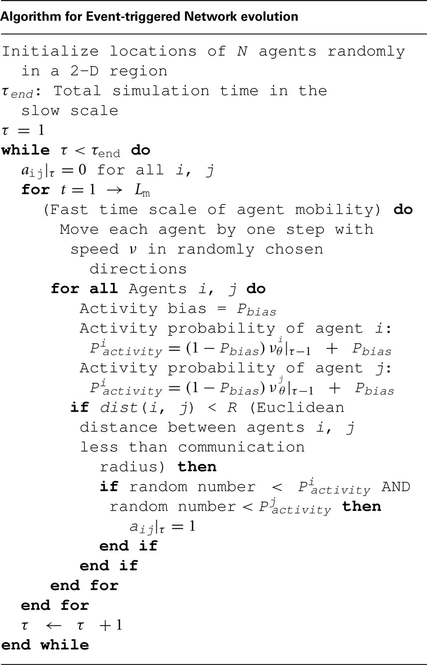
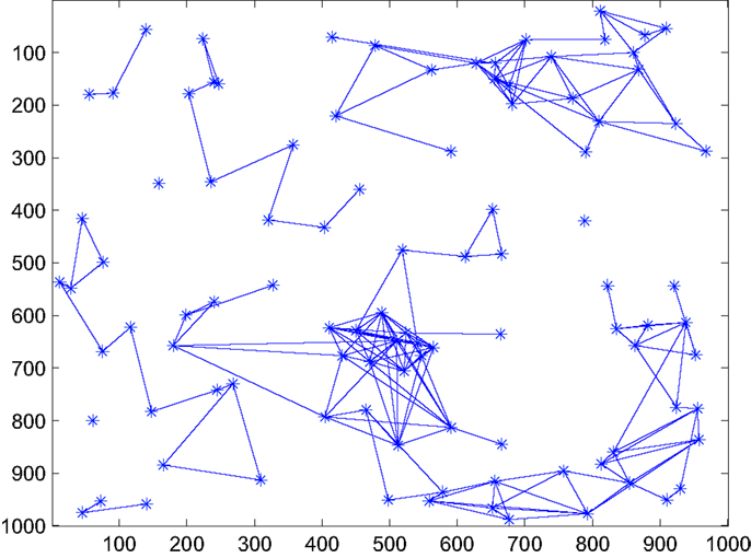
Figure 1. Snapshot of network connectivity in the absence of a hotspot under original formulation, i.e., with P_bias = 1.

FIGURE 2

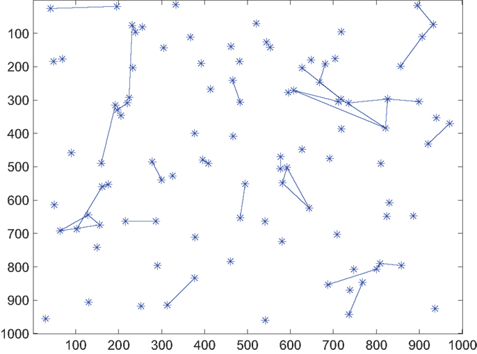
Figure 2. Snapshot of network connectivity in the absence of a hotspot under event-triggered formulation with P_bias = 0.2 C.

Based on the algorithm above, the vector form of information dynamics (see equation (2)) can be modified as

${\mathrm{\nu }}_{\mathrm{\theta }}{|}_{\mathrm{\tau }+1}=\left(1-\mathrm{\theta }\right)\tilde{\mathrm{\Pi }}{|}_{\mathrm{\tau }}{\mathrm{\nu }}_{\mathrm{\theta }}{|}_{\mathrm{\tau }}+\mathrm{\theta \chi }{|}_{\mathrm{\tau }}$ (8)

where, $\tilde{\mathrm{\Pi }}{|}_{\mathrm{\tau }}$ is the modified agent interaction matrix and is a function of ${\mathrm{\nu }}_{\mathrm{\theta }}{|}_{\mathrm{\tau }-1}.$ For analysis purpose, let $\tilde{A}$ be the modified adjacency matrix of the time-varying graph $\tilde{G}$ formed under the event-triggered formulation. Similarly, the modified Laplacian matrix is denoted by $\tilde{\mathcal{L}}$ that can be expressed as

$\tilde{\mathcal{L}}=\tilde{D}-\tilde{A}$

where the modified degree matrix is denoted by $\tilde{D}.$

Note, under the original formulation an element a_ij of the adjacency matrix A is 1 if agents i and j come within the radius of communication or zero otherwise. Now under the event-triggered formulation, if two agents are outside the radius of communication (i.e., a_ij = 0), then the element $\widetilde{a_{\mathit{ij}}}$ of adjacency matrix $\tilde{A}$ is also equal to 0. However, in the other case an element $\widetilde{a_{\mathit{ij}}}$ of $\tilde{A}$ is scaled by the probability that both agents i and j are active simultaneously for at least one epoch in the fast time scale. Let the probability that both agents i and j are active (at least once) at the same time within one message lifetime L_m be denoted by $P_{\mathit{activity}}^{\mathit{ij}}.$ With this setup, the probability that agents i and j are not active simultaneously within a message lifetime L_m is ${\left(1-P_{\mathit{activity}}^i{P}_{\mathit{activity}}^j\right)}^{l_m}.$ Here, l_m is an integer that denotes the number of fast scale epochs (within the message lifetime) during which the agent i and j are close enough to communicate. Since a_ij = 1, there must be at least one fast time epoch during which the agents i and j are within communication radius during one message lifetime L_m. Thus,

$1\le l_m\le L_m$ (9)

Hence,

${\mathcal{P}}_{\mathit{activity}}^{\mathit{ij}}=1-{\left(1-P_{\mathit{activity}}^i{P}_{\mathit{activity}}^j\right)}^{l_m}$

and

$\widetilde{a_{\mathit{ij}}}={\mathcal{P}}_{\mathit{activity}}^{\mathit{ij}}{a}_{\mathit{ij}}$

An extreme case is observed when the adjacency matrix is most sparse or all the agents are at their least possible level of activity, i.e., $P_{\mathit{activity}}^i=P_{\mathit{bias}}\forall i.$ Under this condition, let $P_{\mathit{activity}}^{\mathit{ij}}\forall i,j$ be denoted by Q_bias, i.e.,

${\mathcal{Q}}_{\mathit{bias}}=1-{\left(1-P_{\mathit{bias}}{P}_{\mathit{bias}}\right)}^{l_m}$ (10)

Therefore, with the least activity level of agents the modified Laplacian matrix (denoted by L_min) can be expressed as a scaled version of the Laplacian matrix under the original formulation as follows:

${\mathcal{L}}_{\mathit{min}}={\mathcal{Q}}_{\mathit{bias}}\mathcal{L}$ (11)

Furthermore, in general

$\tilde{\mathcal{L}}={\mathcal{L}}_{\mathit{min}}+{\mathcal{L}}_{\mathrm{\delta }}$ (12)

where ${\mathcal{L}}_{\mathrm{\delta }}$ is a non-zero matrix when agents are more active than their least possible level. Note, both ${\mathcal{L}}_{\mathit{min}}$ and ${\mathcal{L}}_{\mathrm{\delta }}$ are positive semi-definite matrices following the property of Laplacian matrices. Finally, the modified agent interaction matrix $\tilde{\mathrm{\Pi }}{|}_{\mathrm{\tau }}=I-\mathrm{\beta }\tilde{\mathcal{L}}$ remains stochastic and symmetric with proper choice of β as discussed earlier. This property will be useful to obtain certain analytical results for the system.

For the case of congruous time scale (CTS), where the agents’ mobility and information dynamics are comparable, the smallest possible value of ${\mathcal{Q}}_{\mathit{bias}}$ (denoted as ${\mathcal{Q}}_{\mathit{CTS}}$) is observed when l_m = 1.

${\mathcal{Q}}_{\mathit{CTS}}=1-\left(1-P_{\mathit{bias}}{P}_{\mathit{bias}}\right)=P_{\mathit{bias}}^2$ (13)

On the contrary, for the disparate time scale (DTS), the agents’ positions are invariant over the message lifetime. This implies that if two agents are within communication radius, they would remain so during the lifetime of the message (i.e., l_m = L_m). Consequently, the smallest possible value of ${\mathcal{Q}}_{\mathit{bias}}$ (denoted as ${\mathcal{Q}}_{\mathit{DTS}}$) is given as

${\mathcal{Q}}_{\mathit{DTS}}=1-{\left(1-P_{\mathit{bias}}{P}_{\mathit{bias}}\right)}^{L_m}$ (14)

3.1. Convergence of Measure Average

Recall that in original formulation, the steady-state expected measure average (over agents) converges to the steady-state expected state average (over agents) as given by equation (4). The critical property that the proof (see Sarkar et al. (2013) for details) of this relation uses is that Π|_τ is doubly stochastic. Therefore, following the exact same procedure one can show that the same relationship is valid for the modified formulation as well, i.e.,

$E\left[{\mathbb{M}}_a\left({\mathrm{\nu }}_{\mathrm{\theta }}\right)\right]=E\left[{\mathbb{M}}_a\left(\mathrm{\chi }\right)\right]$ (15)

Furthermore, following equation (7) (with k = 1 − P_bias) the steady-state expected (communication) activity average (over agents) denoted by E[𝕄_a(P_activity)] can be expressed as

$E\left[{\mathbb{M}}_a\left(P_{\mathit{activity}}\right)\right]=\left(1-P_{\mathit{bias}}\right)E\left[{\mathbb{M}}_a\left({\mathrm{\nu }}_{\mathrm{\theta }}\right)\right]+P_{\mathit{bias}}$ (16)

Using equation (15), the above equation is rewritten as

$E\left[{\mathbb{M}}_a\left(P_{\mathit{activity}}\right)\right]=\left(1-P_{\mathit{bias}}\right)E\left[{\mathbb{M}}_a\left(\mathrm{\chi }\right)\right]+P_{\mathit{bias}}$ (17)

From this result, it is evident that without the presence of any hotspot (i.e., E[𝕄_a(χ) = 0), the activity remains significantly low (with P_bias being very small). In order to quantify this energy saving, a notion of false alarm is introduced. Let f be defined as the false alarm rate for an individual sensor (agent), i.e., the probability of producing a false alarm in a given fast time epoch. The expected value of the state characteristic function for an agent i is given as

$E\left[{\mathrm{\chi }}^i\right]=\mathit{Prob}\left[{\mathrm{\chi }}^i=1\right]=1-{\left(1-f\right)}^{L_m}$ (18)

where, L_m is the message lifetime. Further, the order of the expectation and the averaging over agents could be switched to obtain

$E\left[{\mathbb{M}}_a\left(\mathrm{\chi }\right)\right]={\mathbb{M}}_a\left(E\left[{\mathrm{\chi }}^i\right]\right)=1-{\left(1-f\right)}^{L_m}$ (19)

Hence, using equation (17), the nominal (i.e., with no hotspots) average communication activity for the network is independent of θ and is given by

$E\left[{\mathbb{M}}_a\left(P_{\mathit{activity}}\right)\right]=\left(1-P_{\mathit{bias}}\right)\left(1-{\left(1-f\right)}^{L_m}\right)+P_{\mathit{bias}}$ (20)

Similar to the original formulation, it is also clear from equation (8) that the temporal dynamics depends on the largest Eigenvalue of $\left(1-\mathrm{\theta }\right)\tilde{\mathrm{\Pi }}{|}_{\mathrm{\tau }}.$ Since $\tilde{\mathrm{\Pi }}{|}_{\mathrm{\tau }}$ is a stochastic matrix, Perron–Frobenius theorem ensures that its largest Eigenvalue is 1; thus, the largest Eigenvalue of $\left(1-\mathrm{\theta }\right)\tilde{\mathrm{\Pi }}{|}_{\mathrm{\tau }}$ is (1 − θ). Therefore, it is expected that the convergence time will increase with decrease in θ. Moreover, first order dynamics should be observed in the time evolution of average ν; this can be attributed to the uniqueness of the largest Eigenvalue of $\tilde{\mathrm{\Pi }}.$ Note, this temporal characteristics of measure average is exactly same as it was for the original formulation.

3.2. Convergence of Measure Variance

Based on the discussion above, it appears that the gain in energy saving does not have any penalizing effect on measure average or its temporal convergence property. However, the measure variance may get affected by the energy aware formulation. Note (from equations (5) and (6)), in both CTS and DTS cases, lower bounds on measure variance only depend on θ and upper bounds on θ and second largest Eigenvalue of (E[(Π|_τ)^T(Π|_τ)]) and Π, respectively. Hence, as the event-triggered formulation modifies the agent interaction matrix to $\tilde{\mathrm{\Pi }}{|}_{\mathrm{\tau }}$ the upper bounds on variance may change. More specifically, the second largest Eigenvalue of $E\left[{\left(\tilde{\mathrm{\Pi }}{|}_{\mathrm{\tau }}\right)}^T\left(\tilde{\mathrm{\Pi }}{|}_{\mathrm{\tau }}\right)\right]$ or $\tilde{\mathrm{\Pi }}{|}_{\mathrm{\tau }}$ depend on second smallest Eigenvalue of the Laplacian Matrix $\tilde{\mathcal{L}}$ (smallest Eigenvalue always being zero for a Laplacian matrix). Recall equation (12) where $\tilde{\mathcal{L}}$ is expressed as a sum of two positive semi-definite, symmetric (Laplacian) matrices ${\mathcal{L}}_{\mathit{min}}$ and ${\mathcal{L}}_{\mathrm{\delta }}$. Therefore, by the Courant-Weil Inequalities, the following can be obtained

${\underset{¯}{\lambda }}_2\left(\tilde{\mathcal{L}}\right)\ge {\underset{¯}{\lambda }}_2\left({\mathcal{L}}_{\mathit{min}}\right)$ (21)

where ${\underset{¯}{\lambda }}_2(X)$ is the second smallest Eigenvalue of matrix X. Thus, the second largest Eigenvalue of $\tilde{\mathrm{\Pi }}{|}_{\mathrm{\tau }}=I-\mathrm{\beta }\tilde{\mathcal{L}}$ will be less than or equal to that of I − βℒ_min, which signifies the worst case performance scenario when all the agents are at their least possible level of activity P_bias. Furthermore, equations (5) and (6) suggest that higher second largest Eigenvalue of agent interaction matrix leads to higher upper bound for measure variance. With this result, it is clear that the upper bound analysis under the worst case performance condition provides a conservative estimate. The following discussion presents upper bound analysis under the worst case performance condition for both DTS and CTS cases.

As discussed earlier, the modified Laplacian matrix $\left(\tilde{\mathcal{L}}\right)$ under the worst case performance condition is given by (see equation (11))

$\tilde{\mathcal{L}}={\mathcal{L}}_{\mathit{min}}={\mathcal{Q}}_{\mathit{bias}}\mathcal{L}$ (22)

where the multiplier Q_bias denotes the probability that two agents are active together within one message lifetime. The stochastic agent interaction matrix $\tilde{\mathrm{\Pi }}$ is given by

$\begin{array}{ccc}\hfill \tilde{\mathrm{\Pi }}& =I-\mathrm{\beta }\tilde{\mathcal{L}}\hfill & \hfill \\ \hfill & =I-\mathrm{\beta }{\mathcal{Q}}_{\mathit{bias}}\mathcal{L}\hfill \\ \hfill & =I-{\mathcal{Q}}_{\mathit{bias}}\left(I-\mathrm{\Pi }\right)\hfill \\ \hfill & ={\mathcal{Q}}_{\mathit{bias}}\mathrm{\Pi }+\left(1-{\mathcal{Q}}_{\mathit{bias}}\right)I\hfill \\ \hfill \end{array}$ (23)

where Π is the agent interaction matrix under the original formulation.

Using the equation above, the second largest Eigenvalue of $\tilde{\mathrm{\Pi }}$ denoted by $\widetilde{{\mathrm{\lambda }}_2}$ can be expressed in terms of the second largest Eigenvalue of Π denoted by λ₂ as

$\widetilde{{\mathrm{\lambda }}_2}={\mathcal{Q}}_{\mathit{bias}}{\mathrm{\lambda }}_2+\left(1-{\mathcal{Q}}_{\mathit{bias}}\right)$ (24)

With this setup, it is straightforward to obtain variance upper bound in the Disparate Time Scale (DTS) case of agent motion and agent communication. Following equation (6), the bounds on the variance ratio (of beliefs ν to observations χ) under the event-triggered formulation are given as

${\mathrm{\theta }}^2\le \frac{{\mathbb{V}}_a\left[{\mathrm{\nu }}_{\mathrm{\theta }}\right]}{{\mathbb{V}}_a\left[\mathrm{\chi }\right]}\le \frac{{\mathrm{\theta }}^2}{{\left[1-\left(1-\mathrm{\theta }\right)\widetilde{{\mathrm{\lambda }}_2}\right]}^2}$ (25)

Furthermore, using equation (24) and replacing ${\mathcal{Q}}_{\text{bias}}$ with ${\mathcal{Q}}_{\text{DTS}}$, the upper bound can be expressed in terms of ${\mathcal{Q}}_{\text{DTS}}$ (a function of the probability of bias P_bias and message lifetime L_m) and the second largest Eigenvalue of the agent interaction matrix Π (i.e., λ₂) as

${\mathrm{\theta }}^2\le \frac{{\mathbb{V}}_a\left[{\mathrm{\nu }}_{\mathrm{\theta }}\right]}{{\mathbb{V}}_a\left[\mathrm{\chi }\right]}\le \frac{{\mathrm{\theta }}^2}{{\left[1-\left(1-\mathrm{\theta }\right)\left(Q_{\mathit{DTS}}{\mathrm{\lambda }}_2+\left(1-Q_{\mathit{DTS}}\right)\right)\right]}^2}$ (26)

where ${\mathcal{Q}}_{\text{DTS}}$ is given by equation (14).

To obtain similar bound for the case of congruous time scale (CTS), Eigenvalues of $E\left[{\tilde{\mathrm{\Pi }}}^T\tilde{\mathrm{\Pi }}\right]$ need to be analyzed. Starting from equation (23), one can obtain

$\begin{array}{c}\hfill {\tilde{\mathrm{\Pi }}}^T\tilde{\mathrm{\Pi }}={\mathcal{Q}}_{\mathit{bias}}^2{\mathrm{\Pi }}^T\mathrm{\Pi }+2{\mathcal{Q}}_{\mathit{bias}}\left(1-{\mathcal{Q}}_{\mathit{bias}}\right)\mathrm{\Pi }+{\left(1-{\mathcal{Q}}_{\mathit{bias}}\right)}^{2}I\\ \hfill \end{array}$ (27)

Taking expectation on both sides

$\begin{array}{c}\hfill E\left[{\tilde{\mathrm{\Pi }}}^T\tilde{\mathrm{\Pi }}\right]={\mathcal{Q}}_{\mathit{bias}}^{2}E\left[{\mathrm{\Pi }}^T\mathrm{\Pi }\right]+2{\mathcal{Q}}_{\mathit{bias}}\left(1-{\mathcal{Q}}_{\mathit{bias}}\right)E\left[\mathrm{\Pi }\right]+{\left(1-{\mathcal{Q}}_{\mathit{bias}}\right)}^{2}I\\ \hfill \end{array}$ (28)

Let v₂ be the unity norm Eigenvector corresponding to the second largest Eigenvalue of $E\left[{\tilde{\mathrm{\Pi }}}^T\tilde{\mathrm{\Pi }}\right]$ (denoted by $\widetilde{{\Lambda }_2}$). Note that the largest Eigenvalue of $E\left[{\tilde{\mathrm{\Pi }}}^T\tilde{\mathrm{\Pi }}\right]$ is 1 and the corresponding Eigenvector is [1, 1, …, 1]^T. Further, v₂ is orthogonal to [1, 1, …, 1]^T. Multiplying both sides of equation (28) by v₂,

$\begin{array}{cc}\hfill E\left[{\tilde{\mathrm{\Pi }}}^T\tilde{\mathrm{\Pi }}\right]v_2& ={\mathcal{Q}}_{\mathit{bias}}^{2}E\left[{\mathrm{\Pi }}^T\mathrm{\Pi }\right]v_2+2{\mathcal{Q}}_{\mathit{bias}}\left(1-{\mathcal{Q}}_{\mathit{bias}}\right)E\left[\mathrm{\Pi }\right]v_2+{\left(1-{\mathcal{Q}}_{\mathit{bias}}\right)}^2{v}_2\hfill \\ \hfill \end{array}$ (29)

Taking norms on both sides of equation (29),

$\begin{array}{cc}\hfill ∥E\left[{\tilde{\mathrm{\Pi }}}^T\tilde{\mathrm{\Pi }}\right]v_2∥& \le {\mathcal{Q}}_{\mathit{bias}}^2∥E\left[{\mathrm{\Pi }}^T\mathrm{\Pi }\right]v_2∥+2{\mathcal{Q}}_{\mathit{bias}}\left(1-{\mathcal{Q}}_{\mathit{bias}}\right)∥E\left[\mathrm{\Pi }\right]v_2∥+{\left(1-{\mathcal{Q}}_{\mathit{bias}}\right)}^2∥v_2∥\hfill \end{array}$ (30)

However, the left hand side of equation (30) can be simplified as

$∥E\left[{\tilde{\mathrm{\Pi }}}^T\tilde{\mathrm{\Pi }}\right]v_2∥=\widetilde{{\Lambda }_2}$ (31)

Also,

$∥E\left[{\mathrm{\Pi }}^T\mathrm{\Pi }\right]v_2∥\le {\Lambda }_2$ (32)

where Λ₂ is the second largest Eigenvalue of E[Π^TΠ]. Moreover,

$∥E\left[\mathrm{\Pi }\right]v_2∥\le ∥v_2∥=1$ (33)

Therefore, the upper bound of the second largest Eigenvalue $\widetilde{{\Lambda }_2}$ is given by (substituting equations (31), (32), and, (33) in equation (30))

$\begin{array}{cc}\hfill \widetilde{{\Lambda }_2}& \le {\mathcal{Q}}_{\mathit{bias}}^2{\Lambda }_2+2{\mathcal{Q}}_{\mathit{bias}}\left(1-{\mathcal{Q}}_{\mathit{bias}}\right)+{\left(1-{\mathcal{Q}}_{\mathit{bias}}\right)}^2\hfill \\ \hfill \end{array}$ (34)

The above expression simplifies to

$\widetilde{{\Lambda }_2}\le {\mathcal{Q}}_{\mathit{bias}}^2{\Lambda }_2+1-{\mathcal{Q}}_{\mathit{bias}}^2$ (35)

Following equation (5) for the case of Congruous Time Scale (CTS) of agent motion and agent communication, the bounds on the ratio (of variance of beliefs ν to observations χ) under the event-triggered formulation are given as

${\mathrm{\theta }}^2\le \frac{{\mathbb{V}}_a\left[{\mathrm{\nu }}_{\mathrm{\theta }}\right]}{{\mathbb{V}}_a\left[\mathrm{\chi }\right]}\le \frac{{\mathrm{\theta }}^2}{1-{\left(1-\mathrm{\theta }\right)}^2\widetilde{{\Lambda }_2}}$ (36)

Thus, using equation (35) and replacing ${\mathcal{Q}}_{\text{bias}}$ with ${\mathcal{Q}}_{\text{CTS}}$, we obtain bounds on the variance ratio $\frac{{\mathbb{V}}_a{\text{[ν}}_{\text{θ}}\text{]}}{{\mathbb{V}}_a[\chi ]}$ in terms of ${\mathcal{Q}}_{\text{CTS}}$ (a function of the probability of bias P_bias) and the second largest Eigenvalue of E[Π^TΠ], where Π is agent interaction matrix with the assumption that all agents are active at all times, i.e., the original formulation.

${\mathrm{\theta }}^2\le \frac{{\mathbb{V}}_a\left[{\mathrm{\nu }}_{\mathrm{\theta }}\right]}{{\mathbb{V}}_a\left[\mathrm{\chi }\right]}\le \frac{{\mathrm{\theta }}^2}{1-{\left(1-\mathrm{\theta }\right)}^2\left({\mathcal{Q}}_{\mathit{CTS}}^2{\Lambda }_2+1-Q_{\mathit{CTS}}^2\right)}$ (37)

Or, in terms of P_bias (using, equation (13))

${\mathrm{\theta }}^2\le \frac{{\mathbb{V}}_a\left[{\mathrm{\nu }}_{\mathrm{\theta }}\right]}{{\mathbb{V}}_a\left[\mathrm{\chi }\right]}\le \frac{{\mathrm{\theta }}^2}{1-{\left(1-\mathrm{\theta }\right)}^2\left(P_{\mathit{bias}}^4{\Lambda }_2+1-P_{\mathit{bias}}^4\right)}$ (38)

4. Simulation Experiments and Results

This section validates the analytical results obtained in the previous section via numerical simulation experiments. The simulation scenario considers a surveillance and reconnaissance mission for a region of area A = 1000² performed by N = 100 number of mobile agents. Each agent has a radius of communication R = 100. The agents are moving in the region with a 2-D random walk fashion with speed, i.e., displacement per unit time ν = 20. Their individual mission goal is to detect existence of any possible hotspot in the region and communicate the detection information to their neighboring agents. A certain information that an agent wants to communicate based on its recent observation, has a message lifetime L_m = 30 units of the faster time-scale (corresponding to agent motion). Thus, an epoch of the slower time-scale τ spans over L_m units of the faster time-scale. As described earlier, the state characteristic function χⁱ of agent i becomes 1 upon detecting a hotspot; otherwise, χⁱ remains 0. As mentioned earlier, a hotspot (i.e., a region where threats may exist) is modeled as a map for probability of detecting the threat. Probability of detection attains the maximum at the center of the hotspot and decays with distance from the center in a radially symmetric manner (please see Sarkar et al. (2013) for details). Therefore, detection depends on the proximity of the agent to the center of the hotspot. After the expiry of message lifetime L_m, while χ value of an agent resets to 0, agent measure (ν) values are updated based on the agent interaction policy described earlier. The parameters specifically introduced in this new formulation are P_activity (activity probability), P_bias (activity bias probability), k = (1 − P_bias) (proportionality constant for using ν feedback to update P_activity), and f (false alarm rate).

4.1. Activity Reduction

The first analysis performed numerically verifies the relationship obtained between steady state expected activity and false alarm rate as given by equation (20). In a simulation performed without the presence of a hotspot, Figure 3 shows the reduction in communication activity (with P_bias = 0.2) as compared to the original formulation (P_bias = 1). As the probability of false alarms f increases the multi-agent system expends more energy for communication.

FIGURE 3

Figure 3. Reduction in energy spent on communication (with P_bias = 0.2) as compared to original formulation (with P_bias = 1).

4.2. Receiver Operating Characteristics

The individual mission goal of each agent is to detect the existence of any possible hotspot or event in the region and communicate the information to their neighboring agents. Although the state characteristic function χ_i of an agent becomes 1 upon detecting a hotspot (or by false alarm), a decision on the existence of a hotspot is made based on the value of agent’s measure ν. Therefore, to generate the receiver operating characteristics (ROC) curve for the entire sensor network, the following decision model is chosen. The multi-agent system as a whole detects a hotspot if measures (ν) of K or more agents exceed a set threshold ν_thresh Mukherjee et al. (2011). In other words, the belief of at least K agents must indicate the presence of a hotspot. In this example, the value of K is chosen to be 3. Typical values of false alarm rates depend on the application domain, which could range from weather monitoring to undersea surveillance (see Urick (1994)) for analysis of false alarm rates). For the purpose of illustration, P_bias and f are taken as 0.2 and f = 3.33 × 10⁻³, respectively.

Figure 4 depicts the ROC curve that describes the trade-off between probability of detection of the hotspot and the probability of false alarms at every slow time epoch. The ROC curve is computed by the varying the magnitude of ν_thresh from 0 to 1. Further, the ROC computed for a range of values of the parameter θ. Small values of θ yield superior performance in terms of detection probability and false alarms. This is due to the fact that, for a small θ, the value of ν for an agent is close to the spatiotemporal average of the agents’ characteristic function χ. While χ is greatly affected by local false alarms and missed detections, ν provides a spatiotemporally filtered interpretation of χ and is a better suited for decision-making. While decreasing the value of θ improves the ROC, there is also an accompanying increase in time taken for detection of an event and a loss of localization accuracy as discussed earlier. This is due to the fact that a low value of θ causes the dynamics of ν to be sluggish and reduces its variance (across agents). Therefore, θ not only determines the trade-off between Propagation Radius and Localization Gradient the choice of the control parameter but can also be optimized based on a trade-off requirement between the ROC performance and detection time.

FIGURE 4

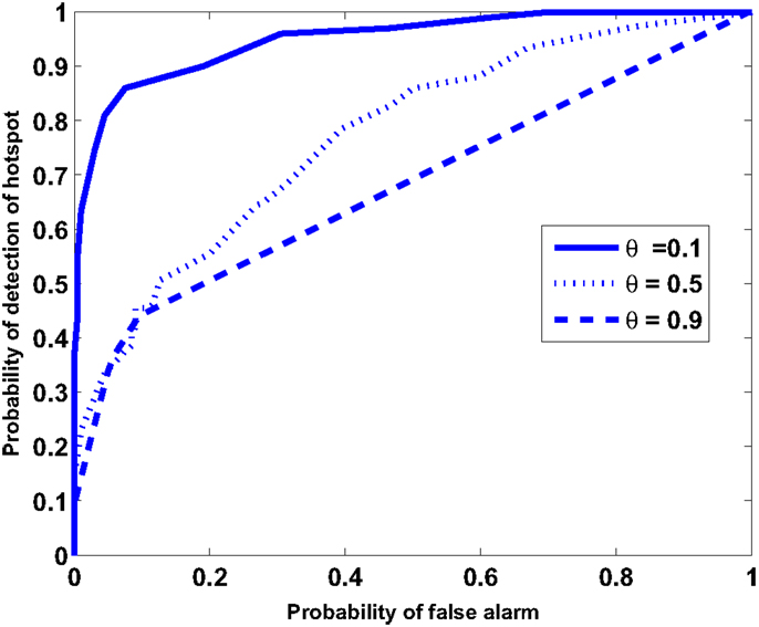
Figure 4. Receiver operating characteristics (ROC) curves under various θ conditions.

Remark 4.1: In the above described simulation, the magnitude of the hotspot (in terms of magnitude and physical range) is an important factor for the ROC. The ROC curve in Figure 4 is constructed for a faint hotspot that covers 0.6% of the area where the maximum probability of detection is 0.5. The probability that an agent performing random walk detects the hotspot at any time is 2.7 × 10⁻³, which is in fact lower than the false alarm rate.

4.3. Convergence of Statistical Moments

Numerical experiments are performed to verify the analytical results related to convergence of statistical moments of measure values. Results are shown for θ = 0.01 for both original and event-triggered formulation. Figure 5 shows that the steady-state expected measure average (over agents) converges to the steady-state expected state average (over agents) irrespective of P_bias values. Temporal characteristics of steady-state expected measure average is also found to be identical for original (P_bias = 1) and event-triggered (P_bias = 0.2) formulations under the same hotspot condition. However, the difference appears in variance characteristics and as suggested in the previous section. As observed in Figure 6, the steady state measure variance increases for decrease in P_bias from 1 to 0.2. Detail validation experiments to verify the new analytically obtained bounds for the event-triggered formulation under both CTS and DTS cases remain an important future work.

FIGURE 5

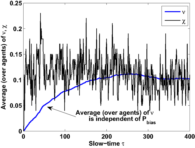
Figure 5. Temporal characteristics of steady-state expected measure average: identical for both original and event-triggered formulations.

FIGURE 6

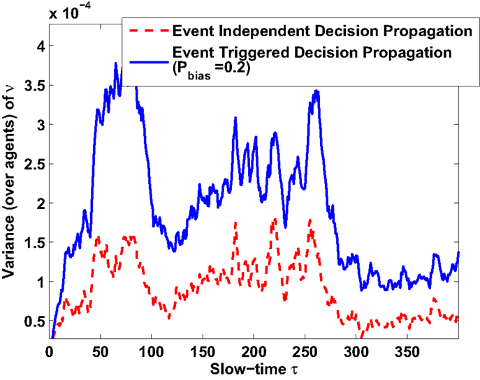
Figure 6. Temporal characteristics of steady-state expected measure variance: variance increases for decrease in P_bias from 1 to 0.2.

4.4. Effect of Spatial Distribution of Agents

Finally, simulations are performed to analyze the effect of the spatial distribution of the agents on the ratio of the variances (belief ν to observation χ) as defined by equation (26). Two spatial distributions are chosen for the simulation, namely, (a) uniform agent densities as well as (b) Gaussian density of agent. The agents’ dynamics is assumed to belong to the DTS type where agents update their states at a much faster timescale as compared to their motion. Figure 7 shows the comparison of ratio of variances obtained as a function of the second largest eigenvalue of agent interaction matrix Λ₂(Π). For the simulation, the value of Λ₂(Π) is varied by modifying the communication radius of the agents. As the communication radius is reduced, the agent interaction reduces leading to a larger second Eigenvalue Λ₂ (slower dynamics). The result shows that the nature of distributions of agents has little effect on the ratio of variances given that the second Eigenvalue of the agent interaction matrix is held fixed.

FIGURE 7

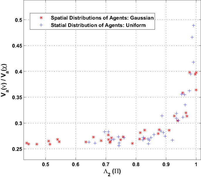
Figure 7. Comparison of ratio of variance (belief ν to observation χ) for different (uniform and Gaussian) spatial distribution of agents.

5. Summary, Conclusion, and Future Work

This paper proposes an energy aware formulation of the generalized gossip policy for distributed decision propagation in mobile sensor networks. The key idea is to conserve energy spent on communication (message transmission and reception) when there is no event of interest in the region of surveillance. The idea is implemented by using an agent’s belief measure as feedback to change its probability of (communication) activity. As a consequence, the time-varying network remains extremely sparse when there is no hotspot and becomes heavily connected when a hotspot appears in the region of surveillance. Analysis and numerical experiments show that the first moment characteristics of agent belief propagation remain same as it was in the original formulation. However, the second moment characteristics changes and as expected information propagation suffers from reduced activity of agents. Still a minimum required level of propagation characteristics can be maintained by choosing a proper value of P_bias. In this context, the analytical results presented in this paper can be used as a guideline for choosing this parameter to obtain a desired trade-off between energy saving potential and decision-making capability of a mobile sensor network. Effects of false alarms on network formation and communication activity are also investigated.

It should be noted that the collaborative decision framework presents a different problem formulation and solution approach compared to those exist in literature today. Specifically, (i) typical source seeking problems (Atanasov et al., 2012; Berdahl et al., 2013) are formulated in a way such that mobile sensors detect a hotspot of interest in the region and try to move toward that. However, the current setup does not require the agents to move toward the source. Apart from computational advantages, this is also particularly more suited in an adverse dynamics environment. In such a case, the network may need to handle multiple non-collocated sources with possible presence of dummy sources. (ii) In many studies (such as Atanasov et al. (2012); Han and Chen (2014)), long-range sensing is considered and source locating algorithms use quantities such as signal strength. However, in real-life scenarios (especially in undersea environment) such a requirement may be very unrealistic, and therefore, the present formulation may be more suited in those cases. (iii) Finally, the analytical results are obtained without specific structural constraints on the underlying network topology, which evolves naturally from agent movements. Therefore, this setup may have more applicability to real-life ad hoc mobile sensor network scenarios.

While detail validation experiments to verify the bounds on variance ratio for the event-triggered formulation under both CTS and DTS cases are currently being pursued, a couple of other important research directions are mentioned below.

1. In the original formulation, it was found that the generalization parameter θ controls the fundamental trade-off between Propagation Radius and Localization Gradient. In the current study, it is found that θ can control the impact of false alarms and detection time as well. Therefore, future work will be devoted to formulate an optimization problem for selection of θ given mission objective and sensing quality.

2. Mobile ad hoc sensor network policies presented here may be particularly relevant in situations where long-range communication or GPS capabilities are very limited and unreliable. In these scenarios, mobile sensor networks can guide neutralizing agents (e.g., in military applications) or other vehicles (e.g., in environmental applications) to reach or avoid various kinds of hotspots present in the environment. Therefore, research is currently being pursued to identify ways that path planning algorithms can exploit distributed decision propagation capabilities.

3. The present formulation uses a feedback of agent belief as a mechanism to control the underlying dynamic communication graph. While this study focuses on how such feedback has the potential to save power consumption in the network, future work will investigate the other (potentially negative) impacts of the belief dynamics, such as network fragmentation.

Conflict of Interest Statement

The authors declare that the research was conducted in the absence of any commercial or financial relationships that could be construed as a potential conflict of interest.

References

Atanasov, N., Le Ny, J., Michael, N., and Pappas, G. J. (2012). “Stochastic source seeking in complex environments,” in 2012 IEEE International Conference on Robotics and Automation (ICRA) (Saint Paul, MN: IEEE), 3013–3018. doi: 10.1109/ICRA.2012.6225289

CrossRef Full Text | Google Scholar

Baras, J. S., and Jiang, T. (2005). “Cooperation, trust and games in wireless networks,” in Advances in Control, Communication Networks, and Transportation Systems (Boston, MA: Birkhuser), 183–202.

Google Scholar

Berdahl, A., Torney, C. J., Ioannou, C. C., Faria, J. J., and Couzin, I. D. (2013). Emergent sensing of complex environments by mobile animal groups. Science 339, 574–576. doi:10.1126/science.1225883

Pubmed Abstract | Pubmed Full Text | CrossRef Full Text | Google Scholar

Choi, H.-L., and How, J. P. (2011). Coordinated targeting of mobile sensor networks for ensemble forecast improvement. IEEE Sens. J. 11, 621–633. doi:10.1109/JSEN.2010.2053197

CrossRef Full Text | Google Scholar

Gonzalez, M. C., Linda, P. G., and Herrmann, H. J. (2006). Networks based on collisions among mobile agents. Physica D 224, 137–148. doi:10.1016/j.physd.2006.09.025

CrossRef Full Text | Google Scholar

Han, J., and Chen, Y. (2014). Multiple UAV formations for cooperative source seeking and contour mapping of a radiative signal field. J. Intell. Rob. Syst. 74, 323–332. doi:10.1007/s10846-013-9897-4

CrossRef Full Text | Google Scholar

Lehning, M., Dawes, N., Bavay, M., Parlange, M., Nath, S., and Zhao, F. (2009). “Instrumenting the earth: next-generation sensor networks and environmental science,” in The Fourth Paradigm: Data-Intensive Scientific Discovery, eds T. Hey, S. Tansley, and K. Tolle (Redmond, WA: Microsoft Research), 45–51.

Google Scholar

Mazo, M., and Tabuada, P. (2008). “On event-triggered and self-triggered control over sensor/actuator networks,” in 2008 47th IEEE Conference on Decision and Control (CDC) (Cancun: IEEE), 435–440. doi:10.1109/CDC.2008.4739414

CrossRef Full Text | Google Scholar

Molavi, P., Jadbabaie, A., Rad, K., and Tahbaz-Salehi, A. (2013). Reaching consensus with increasing information. IEEE J. Sel. Top. Signal Process. 7, 358–369. doi:10.1109/JSTSP.2013.2246764

CrossRef Full Text | Google Scholar

Mukherjee, K., Ray, A., Wettergren, T. A., Gupta, S., and Phoha, S. (2011). Real-time adaptation of decision thresholds in sensor networks for detection of moving targets. Automatica 48, 185–191. doi:10.1016/j.automatica.2010.10.031

CrossRef Full Text | Google Scholar

Patterson, S., Bamieh, B., and El Abbadi, A. (2010). Convergence rates of distributed average consensus with stochastic link failures. IEEE Trans. Automat. Contr. 55, 880–892. doi:10.1109/TAC.2010.2041998

CrossRef Full Text | Google Scholar

Salhieh, A., and Schwiebert, L. (2004). Power-aware metrics for wireless sensor networks. Int. J. Comput. Appl. 26, 119–125. doi:10.2316/Journal.202.2004.2.204-0554

CrossRef Full Text | Google Scholar

Sarkar, S., Mukherjee, K., and Ray, A. (2013). Distributed decision propagation in mobile-agent proximity networks. Int. J. Control 86, 1118–1130. doi:10.1080/00207179.2013.782511

CrossRef Full Text | Google Scholar

Srivastav, A., Ray, A., and Phoha, S. (2009). Adaptive sensor activity scheduling in distributed sensor networks: a statistical mechanics approach. Int. J. Distrib. Sens. Netw. 5, 242–261. doi:10.1080/15501320802473250

CrossRef Full Text | Google Scholar

Tabuada, P. (2007). Event-triggered real-time scheduling of stabilizing control tasks. IEEE Trans. Automat. Contr. 52, 1680–1685. doi:10.1109/TAC.2007.904277

CrossRef Full Text | Google Scholar

Toroczkai, Z., and Guclu, H. (2007). Proximity networks and epidemics. Physica A 378, 68–75. doi:10.1016/j.physa.2006.11.088

CrossRef Full Text | Google Scholar

Urick, R. (1994). Principles of Underwater Sound, 3rd Edn. New York, NY: McGraw-Hill.

Google Scholar

Wan, P., and Lemmon, M. (2009). “Event-triggered distributed optimization in sensor networks,” in Proceedings of the 2009 International Conference on Information Processing in Sensor Networks (IPSN) (Washington, DC: IEEE Computer Society), 49–60.

Google Scholar

Yildiz, M. E., Acemoglu, D., Ozdaglar, A., and Scaglione, A. (2011). “Diffusion of innovations on deterministic topologies,” in Proceedings of ICASSP (Prague: IEEE). doi:10.1109/ICASSP.2011.5947679

CrossRef Full Text | Google Scholar

Yildiz, M. E., Scaglione, A., and Ozdaglar, A. (2010). “Asymmetric information diffusion via gossiping on static and dynamic networks,” in Proceedings of 49th IEEE Conference on Decision and Control (Atlanta, GA: IEEE), 7467–7472.

Google Scholar