iCub whole-body control through force regulation on rigid non-coplanar contacts

1. Introduction

Classical industrial applications employ robots with limited mobility. Consequently, assuming that the robot is firmly attached to the ground, interaction control (e.g., manipulation) is usually achieved separately from whole-body posture control (e.g., balancing). Foreseen applications involve robots with augmented autonomy and physical mobility. Within this novel context, physical interaction influences stability and balance. To allow robots to overcome barriers between interaction and posture control, forthcoming robotics research needs to investigate the principles governing whole-body coordination with contact dynamics, as these represent important challenges toward achieving robot physical autonomy and will therefore be the focus of the present paper.

It is worth recalling that the aforementioned industrial robots have been extensively studied since the early seventies. Robot physical autonomy asks for switching from conventional fixed-base to free-floating robots, whose control has been addressed only during recent years. Free-floating mechanical systems are under actuated and therefore cannot be fully feedback linearized (Spong, 1994). The problem becomes even more complex when these systems are constrained that is their dynamics are subject to a set of (possibly time-varying) non-linear constraints. This is the typical case for legged robots, for which motion is constrained by rigid contacts with the ground.

The major contribution of this work is the implementation and integration of all the building blocks composing a system for balance and motion control of a humanoid robot. The system includes the low-level joint-torque control, the task-space inverse-dynamics control, the task planner and the estimation of contact forces and joint torques. Even though in recent years, other similar systems have been presented (Ott et al., 2011; Herzog et al., 2014), the originality of our contribution lies (i) in the specificities of our test platform and (ii) in a number of design choices that traded off simplicity of implementation for performances of the control system. In particular:

• differently from the other robots, iCub can localize and estimate contact forces on its whole-body thanks to its distributed tactile sensors

• similarly to the DLR-Biped (Ott et al., 2011), iCub is actuated with DC motors and harmonic drives, but we chose to neglect the gear-box flexibility, which simplified the motor-identification procedure and the low-level torque controller

• differently from the above-mentioned platforms, iCub is not equipped with joint-torque sensors, but we designed a method that exploits its internal 6-axis force/torque sensors to estimate the joint torques

• all our control loops run at 100 Hz, which is (at least) 10 times slower with respect to Ott et al. (2011) and Herzog et al. (2014).

We believe that further investigation will be necessary to thoroughly understand all the consequences of our hardware/software design choices. Nonetheless, these peculiarities make the presented system unique, and for this reason we think it is important to share our results with the robotics community.

The paper is organized as follows: Section 2 reviews the state of the art and motivates our specific choices, with a focus on why we defined postural stability by means of the center of pressure at individual contacts. A counterexample discussed in Section 2.3.3 shows that the commonly used global center of pressure is not suitable for the scope of our application. Section 3.1 describes the whole-body distributed force and tactile sensors on iCub. These sensors are used to estimate contact forces (Section 3.2.1), internal torques (Section 3.2.2), and to improve the accuracy of the robot’s inertial parameters (Section 3.3), while Section 3.4 presents the prioritized contact-force controller. Section 4 discusses the implementation scenario, consisting in controlling the iCub posture and contact forces at both arms and feet. Remarkably, iCub can establish and break contacts at the arms using tactile sensing for both contact detection and localization. Finally, Section 5 draws the conclusions.

2. Background

This section reviews previous literature on rigid contacts and their role in whole-body stability. Then we conclude that for the scope of the current paper we need to consider local contact stability as opposed to global stability criteria proposed in previous literature. Section 2.1 makes some general considerations about contacts and Section 2.1.1 gives a characterization of contacts by means of the center of pressure, a point in space that summarizes the effects of distributed forces acting on a rigid body. Section 2.2 focuses on planar unilateral contacts and their stability (Section 2.2.1). This specific type of contacts is associated with a center of pressure that lies on the contact plane (Section 2.2.2). This property is exploited to give necessary and sufficient conditions for the stability of a planar unilateral contact (Section 2.2.3). Section 2.3 reviews previous literature on multiple contacts. In particular, Section 2.3.1 considers the coplanar case, whereas Section 2.3.2 the non-coplanar one. Section 2.3.3 discusses a counterexample to justify our choice of addressing the multiple-contact case without resorting to a global stability criterion as proposed in most of previous approaches. Finally, Section 2.4 briefly reviews the state of the art of prioritized task-space inverse dynamics.

2.1. Contacts

We consider articulated rigid-body systems under the effects of multiple rigid contacts. In general, a contact can be seen as a continuum of infinitesimal forces acting on the surface of a rigid body. The effect of contact forces will be represented with an equivalent wrench w_c = (f_c, μ_c), composed by a three-dimensional force and a three-dimensional torque, denoted f_c and μ_c, respectively. Considering that a contact exerts infinitesimal forces distributed over a surface, f_c is computed as the integral of infinitesimal forces over the surface. Similarly, μ_c is computed as the integral of the infinitesimal torques due to infinitesimal forces over the surface. The effect of other (non-contact) forces and torques acting on the rigid body will be denoted as w_o = (f_o, μ_o), being f_o and μ_o the equivalent force and torque (respectively) resulting from all non-contact forces.

2.1.1. Definition of center of pressure (CoP)

Given a rigid body subject to contact forces, we associate a field of pressure to the contact itself. For each contact point, the pressure is defined as the amount of normal force acting per unit area. The center of pressure (CoP) is defined as an application point where the force obtained by the integration of the field of pressures causes an effect that is equivalent to that of the field of pressures itself. Remark 1: by definition, pressure accounts only for the normal component of the contact forces acting on the surface of a rigid body. Therefore, the CoP comes handy especially when the tangential forces (shear stress) are negligible or does not play a role in the rigid body dynamics (e.g., the effect of tangential forces is compensated by the static friction). Otherwise, the CoP does not represent per se a full characterization of the forces acting on the system and the effect of tangential forces should be also taken into account. Remark 2: at any point in space, the effect of a field of pressures can be represented by an equivalent force and an equivalent torque (the integral of infinitesimal forces and torques, respectively). Given the above definition, the CoP is an application point where the equivalent torque is null.

2.1.2. Existence of the center of pressure (CoP)

Given the above definition, we can infer that the CoP sometimes might not exist. As a trivial example, the CoP does not exist when a field of pressure generates a zero net force but a non-zero net torque. Excluding this trivial case, by resorting to the Poinsot theorem it can be shown (see Appendix A) that the CoP is defined if and only if the resulting net torque is orthogonal to the resulting net force. Two relevant cases that satisfy this condition can be identified: field of pressures due to forces lying on a plane (torques orthogonal to the plane) and field of pressures due to forces orthogonal to a plane (torques lying on the plane). The first is a typical example used in aerodynamics (profile of a wing) and the latter is a typical example in the field of humanoid walking (contact with planar surfaces). In any case, the CoP is never uniquely defined and the set of valid CoPs corresponds to the Poinsot axis (see Appendix A.2). In the case of planar contacts, we will uniquely identify the CoP with the intersection between the axis and the planar contact surface as proposed by Sardain and Bessonnet (2004).

2.2. Planar Unilateral Contact

A particular type of contacts, nominally planar unilateral contacts, has been widely studied to characterize the stability of an articulated rigid-body system while walking on flat terrain. The typical case-study considers a single link (foot) in contact with a flat surface (ground). Proposed stability criteria take into account the fact that while the foot has to be constantly in contact with the ground, the rest of the body is moving and therefore transfers inertial and gravitational forces to the foot. The foot is therefore subject to two sets of wrenches: those due to the contact with the ground (w_c) and those due to the movements of the rest of the body (w_o). For the contact to be stable, these forces should balance (see Section 2.2.1). Force balance might not always hold since planar unilateral contacts exert a limited range of forces and torques. Original stability properties were proposed by Vukobratovic and Juricic (1969), who introduced the zero moment point (ZMP) concept. The ZMP coincides with the unique point on the ground where f_c, μ_c produce zero tangential moments (see Section 2.2.2). As it was pointed out by Sardain and Bessonnet (2004), in the case of planar contacts, the ZMP coincides with the intersection of the Poinsot axis with the contact plane as defined in Section 2.1.1; the ZMP is therefore a valid CoP. Other stability criteria for planar unilateral contacts have been proposed by Goswami (1999) and reviewed in Section 2.2.3.

2.2.1. Definition of stable planar unilateral contact

So far, we have only discussed about forces generated by contacts. In general, contacts also introduce motion constraints and there is always a duality between contact forces and constrained motion. In the case of rigid contacts, the directions in which motion is constrained are precisely those in which (contact) forces can be exerted as observed by Murray et al. (1994). In other words, contact forces and possible motions are always orthogonal. From a control point of view, it is often desirable that the set of motion constraints does not change over time, since if it does, the control problem becomes harder to solve (see, for example, literature on hybrid and switching systems). This is the reason why we say that a contact is stable when the motion constraints induced by it do not change over time. Interestingly, motion constraints are effective on the system only if certain conditions are satisfied. If these conditions are not met (e.g., contact forces violate unilateral constraints or exceed friction cones) contacts are broken and motion constraints are no longer active on the system. It is therefore important to find a set of necessary and sufficient conditions for a contact to constrain always the same motion.

In the case of planar unilateral contacts, these conditions assume an elegant form that will be presented in Section 2.2.3. The analysis is simplified by observing that planar unilateral contacts impose constraints on all linear and angular motions¹. Therefore, a planar unilateral contact imposes null linear and angular accelerations. By means of the Newton–Euler equations on the contact link, motion constraints are therefore guaranteed if and only if f_c = − f_o and μ_c = − μ_o. In a sense, deciding whether or not a planar unilateral contact is stable (with the above terminology) corresponds to understanding if a given wrench f_o, μ_o can be compensated by the forces f_c and torques μ_c generated by the given type of contact. If −f_o, −μ_o lie outside the space of wrenches that a planar unilateral contact can generate, then non-zero accelerations are generated and the contact is broken. The following section shows how to characterize the set of wrenches generated by a planar unilateral contact.

2.2.2. Characterization of the CoP for planar unilateral contacts

Given a planar unilateral contact, the set of forces induced by the contact are such that it is always possible to find a point on the plane where the equivalent moment has null tangential components. This point has been named zero moment point (ZMP) by Vukobratovic and Juricic (1969). The name is sometimes considered misleading [see, for example, Sardain and Bessonnet (2004)] since at the ZMP the “tipping” (or tangential) moment and not the “total” moment is zeroed. The computation of the zero tipping moment point is relatively straightforward and reformulated in Section “Appendix B.1.” In the case of unilateral contacts, the ZMP coincides with the CoP [see Sardain and Bessonnet (2004)] and always lies in the convex hull of the contact points as shown by Wieber (2002) and in Section “Appendix B.1.” It is worth noticing that (in the ZMP context) restricting to tangential moments corresponds (in the CoP context) to neglecting tangential forces (see the first remark in Section 2.1.1).

2.2.3. Characterization of stable planar unilateral contact

Goswami (1999) pointed out that the ZMP lying within the contact convex hull is not a proper stability measure. He therefore formulated some different statements for the characterization of the stability of planar unilateral contacts. These statements make use of the foot rotation indicator (FRI), which corresponds to the unique zero tipping moment point associated to f_o, μ_o and belonging to the contact plane. The name FRI is misleading since this physical quantity can be associated to any rigid body in contact with a planar surface, regardless of the fact that the body itself is a foot or not. Remarkably, the FRI (differently form the CoP) is not constrained in the contact convex hull because f_o and μ_o are not the result of unilateral contact forces. Other names used in literature for the FRI are fictitious ZMP (FZMP) and computed ZMP (CZMP) used by Vukobratovic and Borovac (2004) and Kajita and Espiau (2008), respectively. If the FRI is not within the contact convex hull, Goswami (1999) has shown that a rotation of the rigid link is occurring (i.e., angular acceleration is not identically zero). Vice versa, if the FRI is within the contact convex hull and if frictional constraints are satisfied², then the unilateral contact is stable (i.e., the contact link has null accelerations). The complete proof of the latter statement requires some additional considerations, which are outside the scope of the present paper. The interested reader should refer to chapter 11 of Featherstone (2008).

Both the ZMP and the FRI concept have been used by several authors to define a suitable stability margin for balancing an articulated rigid body system. Hirai et al. (1998) used the ZMP concept to balance one of the earliest versions of the Honda walking humanoids. Huang et al. (2001) adopted a similar concept to define a stability margin tunable by modifying the robot hip motion. Li et al. (1993) used the error between a desired and the computed ZMP to learn stable walking. A good reason to prefer the FRI has been pointed out by Goswami (1999): given that “the ZMP cannot distinguish between the marginal state of static equilibrium and a complete loss of equilibrium of the foot (in both cases, the ZMP is situated at the support boundary), its utility in gait planning is limited. FRI point, on the other hand, may exit the physical boundary of the support polygon and it does so whenever the foot is subjected to a net rotational moment.”

2.3. Multiple Contacts

So far, we discussed the stability of an articulated rigid body system subject to a single planar unidirectional contact. The stability characterization given by Goswami (1999) guarantees contacts stability by requiring the FRI to stay inside the support convex hull. In this section, we review extensions of this criterium to the case of multiple contacts. Proposed extensions search for some global stability criteria to condense the local stability criteria on individual contacts. Section 2.3.1 considers the simple case of multiple coplanar contacts and the associated global stability criteria, known as global CoP. Section 2.3.2 reviews previous literature on global criteria with multiple non-coplanar contacts. The present section concludes by observing that, for the scope of the present paper, it is mandatory to abandon global criteria and stick to local ones. The conclusion follows from a counterexample, provided in Section “Appendix A.2” and discussed in Section 2.3.3.

2.3.1. Multiple coplanar contacts

In this section, we consider the case of articulated rigid body systems in contact with a flat surface (typically the ground). Differently from the previous sections, we assume that more than one single rigid body is in contact with the flat ground and therefore we consider a multiple coplanar contacts scenario. Within this context, we distinguish between local CoP (one per each rigid body in contact with the ground) and global CoP (the center of pressure resulting from all rigid bodies in contact). The local CoP of a rigid body has been defined and characterized in Sections 2.1.1, 2.2.2, and 2.2.3. These definitions and characterizations refer to a single rigid body (e.g., the foot) but can be extended to any rigid body of the articulated system. Computations in this case account only for the contact forces acting on the rigid body itself. Global CoP (GCoP) is instead a quantity associated with the whole articulated system and corresponds to the center of pressure obtained by integrating all contact forces acting on the articulated system. Most of the previous literature does not distinguish between local and global center of pressure but often refer to the latter when characterizing stability during the double-support phase of flat terrain walking. Remarkably, the property of the GCoP lying inside the contacts convex hull still holds. This stability criterion has been used by several authors (Huang et al., 2001; Wieber, 2002; Stonier and Kim, 2006) to infer stability in flat terrain walking. In particular, Wieber (2002) defined a motion to be realizable if and only if the GCoP lies inside the convex hull of contact points. Even though Popovic and Herr (2005) questioned the use of the GCoP as a way to guarantee postural stability, associated criteria are at present the most adopted for planning walking trajectories. In Section 2.3.3, we further question the GCoP as a stability criterion, focusing in particular on the scope of the current paper.

2.3.2. Mutiple non-coplanar contacts

Harada et al. (2003) defined a generalized ZMP (GZMP) and a projected convex hull to formulate stability conditions for a limited class of arm/leg coordination tasks. Sardain and Bessonnet (2004) proposed a concept of virtual surface and virtual CoP-ZMP limited to the case of two non-coplanar contacts. In spite of the adopted simplification, authors themselves admit their failure in finding an associated pseudo support polygon onto which the pseudo-ZMP stays. Hyon et al. (2007) presented a framework for computing joint torques that optimally distributes forces across multiple contacts; conditions for the CoP to lie within the supporting convex hull are formulated but stability conditions are not formulated with sufficient level of details.

2.3.3. Global versus local CoP

In the present paper, we formulate a whole-body postural control, which assumes stable contacts. Stability, as defined in Section 2.2.1 guarantees time invariance of motion constraints and avoids the complications of controlling hybrid systems. Necessary and sufficient conditions for stability of individual contacts can be obtained by resorting to the FRI of each contact. Most of previous literature on flat terrain walking postulates the GCoP to lie in the contacts convex hull as a stability criterium. This criterium is a necessary and sufficient condition for a whole-body motion to be realizable as pointed out by Wieber (2002) (see, in particular, Section 3.2 of his paper). However, it is not a sufficient condition to guarantee stability of all contacts. Section “Appendix B” provides a counterexample in the simple case of two coplanar contacts: the GCoP is shown to lie in the contacts convex hull but individual contacts are proven to be unstable. We therefore decide in this paper to stick to local contact stability criteria since no previous global criteria guarantee the stability of all local contacts.

2.4. Task-Space Inverse Dynamics

We now briefly review the vast literature on prioritized task-space inverse-dynamics control and we motivate our choices in this regard. Sentis (2007) and Park (2006) have been pioneers in the control of articulated free-floating rigid bodies exploiting the operational-space framework (Khatib, 1987). More recent approaches have explored the idea of simplifying the system dynamic equations by performing suitable projections onto the null space of the contact forces as proposed by Righetti et al. (2011) and Aghili (2005). While being computationally efficient (i.e., a total computation time below 1 ms), all these approaches share a common drawback: contact forces cannot be controlled. As a consequence, stability of the contacts cannot be guaranteed, which may lead the robot to tip over and fall.

As opposed to these analytical solutions to the control problem, an alternative numerical approach proposed by de Lasa et al. (2010) is to use a Quadratic Programing solver. This allows to include inequality constraints into the problem formulation, which can model control tasks and physical constraints (e.g., joint limits, motor-torque bounds, force friction cones). Even if this technique can guarantee contact stability, solving a cascade of Quadratic Programs with inequality constraints can be critical from a computational standpoint.

We decided to take an in-between approach: our framework of choice [see Section 3.4 or Del Prete et al. (2014) for details] allows to control the contact forces, but with a computational complexity of the same order of inverse-dynamics-based methods. Compared to optimization-based methods, our implementation does not allow for inequality constraints. To the best of our knowledge, the only real-time implementation of a cascade of Quadratic Programs with inequalities has been tested with a 14-DoF robot on a fast 3.8 GHz CPU (Herzog et al., 2014). We cannot be sure that this method will be fast enough for 26 DoFs and/or a slower CPU. For this reason, while we think that using inequalities could be useful, we postponed it to the (near) future because we know that it demands for an efficient and careful software implementation.

3. Materials and Methods

In this section, we present our approach to solve the problem of controlling whole-body posture on multiple rigid planar contacts. We suppose each contact to be planar, but contact planes to be in general non-coplanar. Within this context, the considerations presented in the previous sections justify our choice to abandon the idea of defining a global stability criterion (such as the GCoP). In case of non-coplanar contacts, a global CoP is not even properly defined given that the resulting force and torque might not in general be orthogonal (see Sections 2.1.2 and Appendix A.2). In any case, the counterexample in Section “Appendix B.1” suggests to consider multiple local stability criteria instead of a single global one. Local contact stability has been defined in Section 2.2.1 and it has been characterized as a condition for motion constraints to be time invariant. At present, necessary and sufficient conditions for contact stability have been formulated only in the case of planar rigid unilateral contacts (see Section 2.2.3). This is the reason why the scope of the current paper is limited to multiple planar contacts on rigid non-coplanar surfaces. Future extensions of the present work are foreseen in the direction of characterizing contact stability in more general situations.

In the rigid and planar contact case, contact stability has been characterized by means of the contact FRI and CoP. Both quantities depend on the wrench (i.e., both force and torque) at the contact point. Assuming that contacts might occur at any point on the robot body, an estimate of the contact wrench might be difficult to obtain if not impossible. Conventional manipulators measure wrenches at the end-effector, where force and torque sensors are placed. Joint-torque sensing gives only an incomplete characterization of contact wrenches. The problem can be solved adopting whole-body distributed force/torque (F/T) and tactile sensors as those integrated in the iCub humanoid (Section 3.1). This specific design choice calls for custom algorithms for contact-wrench estimation (Section 3.2.1), internal torques measurement (Section 3.2.2), and dynamic model identification (Section 3.3). Whole-body control with multiple non-coplanar contacts is discussed in Section 3.4 and requires all the above custom components for its implementation (Section 4).

3.1. Whole-Body Distributed Wrench and Contact Sensing

The platform used to perform experimental tests is the iCub humanoid robot, which is extensively described in Metta et al. (2010). One of the main features of this system is represented by the large variety of sensors, which include whole-body distributed F/T sensors, accelerometers, gyroscopes (see Figure 2), and pressure sensitive skin. Furthermore the robot possesses two digital cameras and two microphones. From a mechanical standpoint, iCub is 104 cm tall and has 53 degrees of freedom: 6 in the head, 16 in each arm, 3 in the torso, and 6 in each leg. All joints but the hands and head are controlled by brushless electric motors coupled with harmonic drive gears. During experimental tests, we mainly exploit two kinds of sensors: the F/T sensors and the distributed sensorized skin. The F/T sensor described in Fumagalli et al. (2012) is a 6-axis custom-made sensor that is mounted in both iCub’s arms between the shoulders and elbows and in both legs between the knees and hip and between the ankles and feet. This solution allows to measure internal reaction forces, which in turn can be exploited to estimate both the internal dynamics and external forces exerted on its limbs. The robot skin (Cannata et al., 2008; Maiolino et al., 2013) is a compliant distributed pressure sensor composed by a flexible printed circuit board (PCB) covered by a layer of three dimensionally structured elastic fabric further enveloped by a thin conductive layer. The PCB is composed by triangular modules of 10 taxels, which act as capacitance gages plus two temperature sensors for drift compensation. In our experiments, iCub’s upper body was wrapped with approximately 2000 sensors, each foot sole is covered with 250 taxels, while 1080 further sensors are at the last design and integration stage on the lower body. Each single taxel has 8 bits of resolution, and measurements can be provided as raw data or as thermal drift compensated.

FIGURE 1

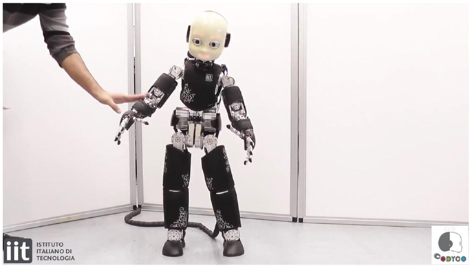
Figure 1. See the video showing the control performances of the control architecture https://www.youtube.com/watch?v=jaTEbCsFp_M.

FIGURE 2

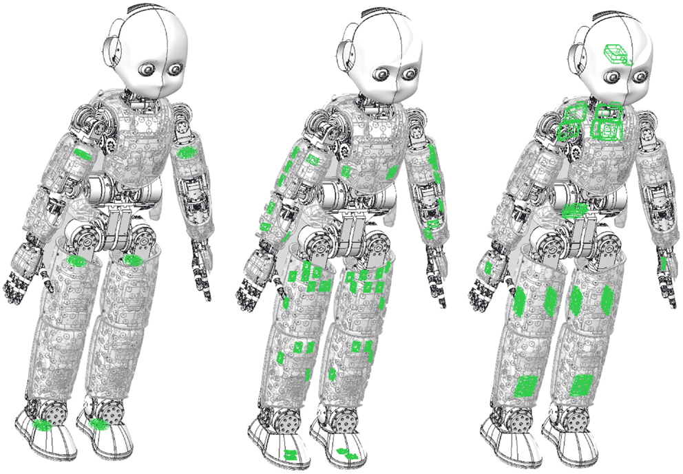
Figure 2. Mechanical schemes of the humanoid robot iCub with force/torque sensors, gyroscopes, and accelerometers highlighted in green. Left: locations of the six proximal six-axis F/T sensors (legs and arms). Center: locations of the skin microcontrollers, which have a 3D accelerometer embedded. Right: locations of the motor microcontrollers and the commercial inertial sensor, with the latter having a 3D gyroscope and a 3D accelerometer embedded.

3.2. Internal and External (Contact) Wrench Estimation

Fumagalli et al. (2012) proposed a theoretical framework that exploits embedded F/T sensors to estimate internal/external forces acting on floating-base kinematic trees with multiple-branches. From a theoretical point of view, the proposed framework allows to virtually relocate the available F/T sensors anywhere along the kinematic tree. The algorithm consists in performing classical recursive Newton–Euler algorithm (RNEA) steps with modified boundary conditions, determined by the contact and F/T sensor location. It can be shown that relocation relies solely on inertial parameters, velocities, and accelerations of the rigid links in between the real and virtual sensors [see, in particular, the experimental analysis conducted by Randazzo et al. (2011)]. The proposed algorithm consists in cutting the floating-base tree at the level of the (embedded) F/T sensors obtaining multiple subtrees as in Figure 3. Then, each subtree is an independent articulated floating-base structure governed by the Newton–Euler dynamic equations. The F/T sensor, gives a direct measurement of one specific external wrench acting on the structure (green arrows in Figure 3). Other external wrenches (red arrows in Figures 3 and 4) can be estimated with the procedure hereafter described.

FIGURE 3

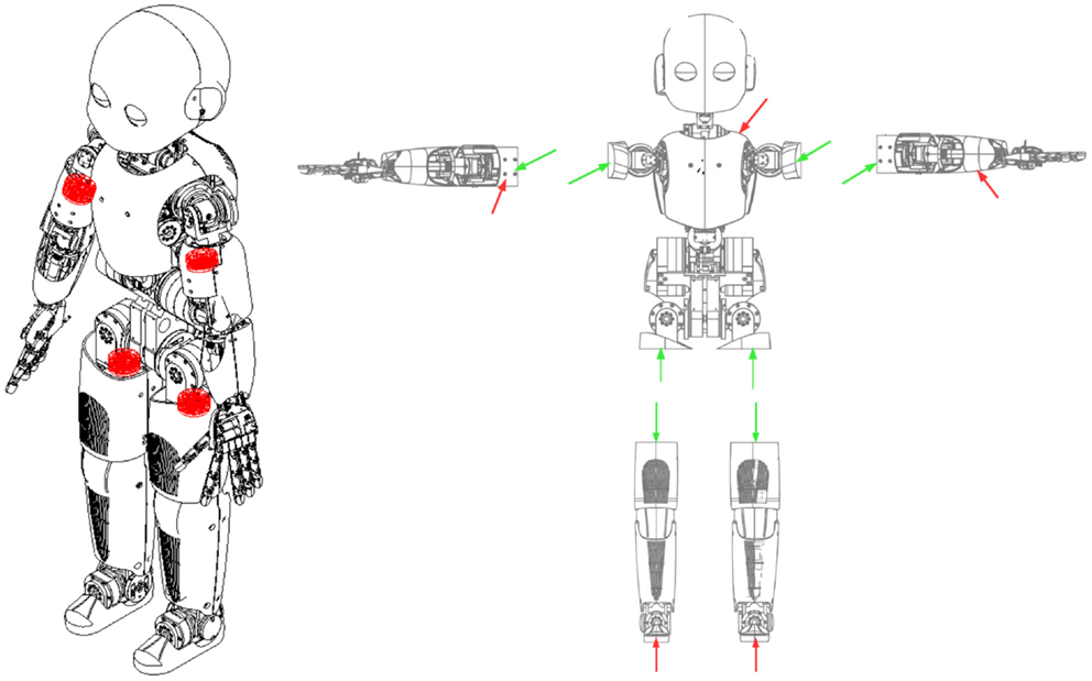
Figure 3. The left picture shows the location of four (out of six) F/T sensors on the iCub humanoid (sensors at the feet are omitted in this picture). The right picture shows the induced iCub kinematic tree partitioning. Each obtained subpart can be considered an independent floating-base structure subject to an external wrench, which coincides with the one measured by the F/T sensor (green arrow). Red arrows represent possible location for the unknown external wrenches.

FIGURE 4

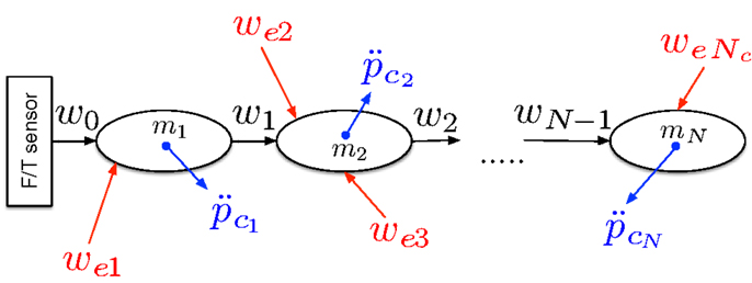
Figure 4. Sketch of a kinematic chain with an embedded F/T sensor. Although the sketch refers to a serial chain, the theoretical framework holds also in the case of multiple-branches articulated chains (see, for example, the torso sub-chain in Figure 3).

3.2.1. Method for estimating external wrenches

We now describe a method for the estimation of contact wrenches; more details can be found in Del Prete et al. (2012). Let us consider a kinematic chain composed by N links, having a F/T sensor at the base (see Figure 4), where w_i is the wrench (i.e., force and moment) exerted from link i to link i + 1, ${\ddot{p}}_{c_i}$ is the acceleration of the center of mass of link i and m_i is the mass of link i. We know w₀ (i.e., the F/T sensor measurement), the K contact locations r_0,ei, … , r_0,eK (i.e., the locations where the skin senses contacts), and we want to estimate the K contact wrenches w_e1, … , w_eK. Writing Newton’s and Euler’s equations for each rigid link and summing up all the N resulting equations we obtain:

$f_0+{\displaystyle \sum _{i=1}^K{f}_{ei}}={\displaystyle \sum _{i=1}^N{m}_i{\ddot{p}}_{c_i},}$ (1)

${\mathrm{\mu }}_0+{\displaystyle \sum _{i=1}^K}\left({\mathrm{\mu }}_{\mathit{ei}}+r_{0,\mathit{ei}}\times f_{\mathit{ei}}\right)={\displaystyle \sum _{i=1}^N}\left(r_{0,c_i}\times m_i{\ddot{p}}_{c_i}+I_i^i{\dot{\mathrm{\omega }}}_i+{\mathrm{\omega }}_i\times I_i^i{\mathrm{\omega }}_i\right),$ (2)

where $I_i^i$ is the inertia of link i, ω_i and ${\dot{\mathrm{\omega }}}_i$ are the angular velocity and acceleration of link i, respectively, and $r_{0,c_i}$ is the vector connecting the chain base to the center of mass of link i. Noting that in equations (1) and (2) the only unknowns are the contact wrenches, the estimation problem may be solved rewriting these equations in matrix form Ax = b, where x ∈ ℝ^u contains all the u contact unknowns, whereas A ∈ ℝ^6×u and b ∈ ℝ⁶ are completely determined. The equations are constructed taking into account the type of possible contacts among the following three: pure wrench (w_e, 6-dimensional vector corresponding to force and torque); pure force (f_e, 3-dimensional vector corresponding to a pure force and no torque); force norm (∥f_e∥, one-dimensional unknown assuming the force to be orthogonal to the contact surface). In the simplest case, only a single contact acts on the sub-chain and the associated pure wrench can be uniquely determined (system of six equations and six unknowns). In other cases, a solution can be obtained with the following least squares procedure. The matrix A is built by attaching columns for each contact according to its type. The columns associated to pure wrenches (A_w), pure forces (A_f), and force norm (A_n) are the following:

$A_w=\left[\begin{array}{cc}\hfill I\hfill & \hfill 0\hfill \\ \hfill S\left(r_{0,\mathit{en}}\right)\hfill & \hfill I\hfill & \hfill \hfill \end{array}\right],A_f=\left[\begin{array}{c}\hfill I\hfill \\ \hfill S\left(r_{0,\mathit{en}}\right)\hfill \end{array}\right],A_n=\left[\begin{array}{c}\hfill {\widehat{u}}_n\hfill \\ \hfill r_{0,\mathit{en}}\times {\widehat{u}}_n\hfill \end{array}\right].$

where S(v) ∈ ℝ^3×3 is the skew-symmetric matrix such that S(v)z = v × z, with × denoting the cross product operator, and ${\widehat{u}}_n$ is the versor of the contact force f_en. The matrix A mainly depends on the skin spatial calibration, which can be obtained and refined with the procedure described by Del Prete et al. (2011). The 6-dimensional vector b is defined as:

$b=\left[\begin{array}{c}\hfill f_b\hfill \\ \hfill {\mathrm{\mu }}_b\hfill \end{array}\right]=\left[\begin{array}{c}\hfill {\displaystyle \sum _{i=1}^N}{m}_i{\ddot{p}}_{c_i}-f_0\hfill \\ \hfill {\displaystyle \sum _{i=1}^N}\left(r_{0,c_i}\times m_i{\ddot{p}}_{c_i}+I_i^i{\dot{\mathrm{\omega }}}_i+{\mathrm{\omega }}_i\times I_i^i{\mathrm{\omega }}_i\right)-{\mathrm{\mu }}_0\hfill \end{array}\right]$

The vector b depends on kinematic quantities, which can be derived for the whole-body distributed gyros, accelerometers, and encoders. Details on how to estimate these quantities have been detailed by Fumagalli et al. (2012). Once A and b have been computed, we can use the equation Ax = b for estimating external wrenches. The equation defines a unique solution if there is exactly one unknown wrench on the considered sub-chain. In the case of interest for the present paper, an exact characterization of the interaction wrenches can be obtained if there exists exactly one contact wrench per each of the sub-chains obtained by the body structure partition induced by the F/T sensor positions (see Figure 3). In all other situations, an exact estimate cannot be obtained but from a procedural point of view it is preferable to give a reasonable estimate of all the contact wrenches. The solution we adopted consists in computing the minimum norm x* that minimizes the square error residual:

$x^{\ast }=A^{†}b$

where A^† is the Moore–Penrose pseudo-inverse of A. The method has been implemented as an extension of the iDyn library³ and it has been integrated with other software modules to create an efficient software system able to estimate internal and external wrenches of the whole iCub robot.

3.2.2. Method for estimating internal torques

Once an estimate of external forces is obtained with the method described in Section 3.2.1, internal wrenches can also be estimated with a standard Newton–Euler force propagation recursion. Projection of the internal wrenches on the joint axes provides an estimate of the joint torques τ. A torque controller with joint friction compensation guarantees that each motor provides the desired amount of torque to the joints. In order to improve the torque tracking performance, a suitable identification procedure was adopted to estimate the voltage to torque transfer function for each motor. Details are given in the following section together with some details on the dynamic model identification.

3.3. Dynamic Model Estimation

As it was previously pointed out, the technology available in the iCub (nominally, whole-body distributed tactile and F/T sensing) and the estimation algorithm presented in the previous sections allows to simultaneously estimate internal (i.e., joint torques) and external (i.e., contact) forces. The accuracy of the estimates is decisive for the efficacy of the control algorithm that will be described in Section 3.4. A key element to improve the estimation and control accuracy is the availability of a reliable dynamic model [masses, inertias, and center of mass positions in equations (1) and (2)]. Standard identification procedures do not apply directly and a customization to iCub specific sensor modalities and distributions is necessary. In the following two subsections, we describe the solution that we implemented in order to improve dynamic model accuracy (Section 3.3.1) and torque tracking performances (Section 3.3.2).

3.3.1. Dynamic model identification

The accuracy of the system dynamics equation (7) is crucial in the proposed control framework since it affects the controller equation (8) and the internal/external torque estimation procedure described in Section 3.2. Individual dynamic parameters (mass, inertia, and center of mass position) of the rigid bodies constituting an articulated chain can be directly obtained from CAD drawings. These parameters are often not sufficiently accurate and standard identification procedures such as those proposed in the handbook of robotics by Hollerbach et al. (2008) can be applied in order to improve modeling accuracy. Remarkably, these procedures do not give an estimate of individual parameters but some linear combination of them, known in literature as the base parameters. It remains therefore to be clarified if the base parameters suffice to implement the procedure described in Section 3.2.1 to estimate external wrenches. This procedure, written as it is, requires the knowledge of individual dynamic parameters as evident from equations (1) and (2). Additionally, it needs to be verified that also the procedure for estimating internal torques presented in Section 3.2.2 can be reformulated in terms of the base parameters only. Interestingly, it can be shown, resorting to the work by Ayusawa et al. (2014) that the base parameters are a subset of those used for both the estimation procedures in Section 3.2.

3.3.2. Modeling and representation of the motor transfer function

Another important component in implementing the control strategy detailed in Section 3.4 is torque control. For the scope of the present paper, it was necessary to implement a model-based controller tuned for each motor. The model assumes that the i-th joint’s torque τ_i is proportional (k_t) to the voltage V_i applied to the associated motor, with the additional contribution of some viscous (k_v) and Coulomb (k_c) friction:

$V_i=k_t{\mathrm{\tau }}_i+\left(k_{\mathit{vp}}s\left({\dot{\mathrm{\theta }}}_i\right)+k_{\mathit{vn}}s\left(-{\dot{\mathrm{\theta }}}_i\right)\right){\dot{\mathrm{\theta }}}_i+\left(k_{\mathit{cp}}s\left({\dot{\mathrm{\theta }}}_i\right)+k_{\mathit{cn}}s\left(-{\dot{\mathrm{\theta }}}_i\right)\right)\text{sign}\left({\dot{\mathrm{\theta }}}_i\right),$ (3)

where ${\dot{\mathrm{\theta }}}_i$ is the motor velocity, s(x) is the step function (1 for x > 0, 0 otherwise) and sign(x) is the sign function (1 for x > 0, −1 for x < 0, 0 for x = 0). Operationally, it was observed quite relevant to distinguish between positive and negative rotations as represented in the model above. We identified the coefficients k_t, k_vp, k_vn, k_cp, k_cn for each joint with an automatic procedure implemented in an open-source software module⁴. The motor controller exploits the transmission model and implements the following control strategy:

$V_i=k_t\left({\mathrm{\tau }}_i^d-k_p\widetilde{{\mathrm{\tau }}_i}-k_i\int \widetilde{{\mathrm{\tau }}_i}\text{dt}\right)+\left[k_{\mathit{vp}}s\left({\dot{\mathrm{\theta }}}_i\right)+k_{\mathit{vn}}s\left(-{\dot{\mathrm{\theta }}}_i\right)\right]{\dot{\mathrm{\theta }}}_i+\left[k_{\mathit{cp}}s\left({\dot{\mathrm{\theta }}}_i\right)+k_{\mathit{cn}}s\left(-{\dot{\mathrm{\theta }}}_i\right)\right]\tanh \left(k_s{\dot{\mathrm{\theta }}}_i\right),$ (4)

where $\tanh \left(k_s{\dot{\mathrm{\theta }}}_i\right)$ is used to smooth out the sign function, k_s is a user-specified parameter that regulates the smoothing action, and ${\tilde{\mathrm{\tau }}}_i={\mathrm{\tau }}_i-{\mathrm{\tau }}_i^d$ is the i-th torque tracking error, and k_p,k_i > 0 are the low-level control gains. The control objective for the torque controller consists in obtaining $\mathrm{\tau }\simeq {\mathrm{\tau }}^d$ and therefore the controller will make the assumption that the commanded value ${\mathrm{\tau }}_i^d$ is perfectly tracked by the torque controller. Also, observe that there is no derivative term in the parenthesis on the right hand side of equation (4). In fact, the measurement of ${\dot{\tilde{\mathrm{\tau }}}}_i$ is noisy and unreliable at the current state of the iCub’s measuring devices.

3.3.3. Differential joint torque and motion coupling

Specific care was posed in controlling the torques at joints actuated with a differential mechanism. As an example, we consider here the torso roll, pitch, and yaw joint represented in Figure 5. In particular, define q ∈ ℝ³ the vector of the joint angles corresponding to the torso yaw, the torso roll, and torso pitch degree of freedom. Also, by abusing notation, define θ ∈ ℝ³ as the angles between the stator and the rotor of the motors 0B4M0, 0B3M0, and 0B3M1. Then, a simple analysis leads to the following relationship:

$\dot{q}=T\dot{\mathrm{\theta }},T=:\left[\begin{array}{ccc}\hfill \frac{r}{R}\hfill & \hfill \frac{r}{2R}\hfill & \hfill \frac{r}{2R}\hfill \\ \hfill 0\hfill & \hfill 0.5\hfill & \hfill 0.5\hfill \\ \hfill 0\hfill & \hfill -0.5\hfill & \hfill 0.5\hfill \\ \end{array}\right],$ (5)

where r and R are the radius of the pulleys sketched in Figure 5. The above matrix T is obtained by combining a classical differential coupling between pitch and yaw (first two rows) with a more complicated coupling with the roll motion (third row, see Figure 6). Defining τ_q to be the link torques and τ_θ the motor torques, the coupling induced on torques can be easily obtained by imposing the equality between link and motor powers:

$\begin{array}{lll}\hfill {\dot{q}}^{\top }{\mathrm{\tau }}_q={\dot{\mathrm{\theta }}}^{\top }{\mathrm{\tau }}_{\mathrm{\theta }}\forall \dot{q},\dot{\mathrm{\theta }}\Rightarrow {\mathrm{\tau }}_q=& T^{-\top }{\mathrm{\tau }}_{\mathrm{\theta }}\text{\hspace{0.17em}with\hspace{0.17em}}{T}^{-\top }:=& \left[\begin{array}{ccc}\frac{R}{r}& 0& 0\\ -1& 1& 1\\ 0& -1& 1\end{array}\right].\end{array}$ (6)

FIGURE 5

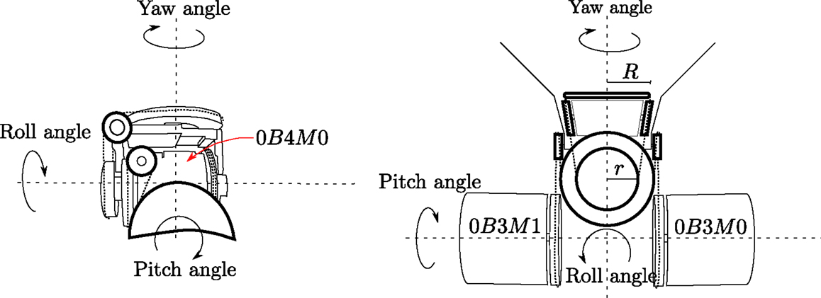
Figure 5. The sketch represents the differential joint of the iCub torso. The pitch, yaw, and roll joints are actuated with three motors 0B4M0, 0B3M0, and 0B3M1 in differential configuration. Motor (θ ∈ ℝ³) and joint (q ∈ ℝ³) positions are coupled as described in Figure 6.

FIGURE 6

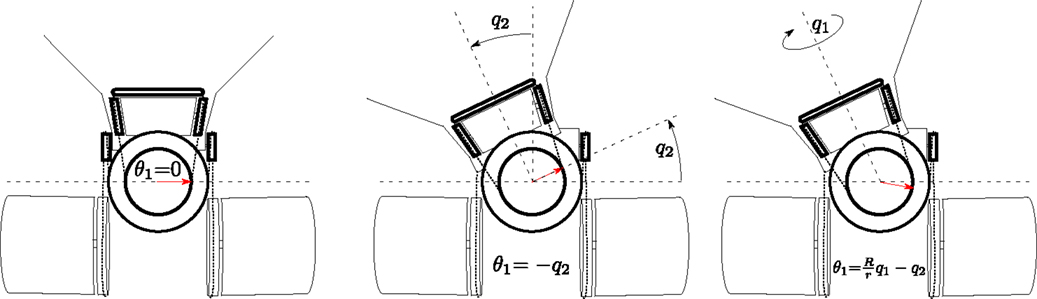
Figure 6. The sketch is used to represent the kinematic coupling between the yaw and roll movements. A roll movement of an angle q₂ implies an equal and opposite movement of the rotor of the motor 0B4M0. This rotor moves, modulo the transmission ratio, also when a yaw movement of an angle q₁ occurs.

In the case of coupled joints, the transformation matrix T is used in both equations (3) and (4), which hold at the motor level. Since position ($\dot{q}$) and torque (τ) feedback is available at the joint level, suitable transformations need to be applied. In the case of coupled joints, our current software⁵ implements joint per joint equations (3) and (4) with substitutions τ ↔ τ_θ and $\dot{q}\leftrightarrow \dot{\mathrm{\theta }}$ where motor velocity ($\dot{\mathrm{\theta }}$) and motor torques τ_θ are obtained from joint velocity ($\dot{q}$) and joint torques (τ_q) as follows:

$\dot{\mathrm{\theta }}=T^{-1}\dot{q},{\mathrm{\tau }}_{\mathrm{\theta }}=T^{\top }{\mathrm{\tau }}_q.$

3.4. Complete Force Control

In this section, we describe the control algorithm for controlling an articulated rigid body subject to multiple rigid constraints. The system dynamics are described by the following constrained differential equations:

$\begin{array}{ll}\hfill \underset{M\left(q\right)}{\underbrace{\left[\begin{array}{cc}{M}_b& M_{\mathit{bj}}\\ M_{\mathit{bj}}^{\top }& M_j& \end{array}\right]}}\underset{\dot{v}}{\underbrace{\left[\begin{array}{c}{\dot{v}}_b\\ {\ddot{q}}_j& \end{array}\right]}}+\underset{h\left(q,v\right)}{\underbrace{\left[\begin{array}{c}{h}_b\\ h_j& \end{array}\right]}}-\underset{J_c{\left(q\right)}^{\top }}{\underbrace{\left[\begin{array}{c}{J}_{\mathit{cb}}^{\top }\\ J_{\mathit{cj}}^{\top }\end{array}\right]}}f& =\underset{S^{\top }}{\underbrace{\left[\begin{array}{c}{0}_{6\times n}\\ I_{n\times n}\end{array}\right]}}\mathrm{\tau }\end{array}$ (7a)

$J_c\left(q\right)\dot{v}+{\dot{J}}_c\left(q,v\right)v=0,$ (7b)

where q ∈ SE(3) × ℝⁿ, with SE(3) the special Euclidian group, represents the configuration of the floating-base system, which is given by the pose of a base-frame [belonging to SE(3)] and n generalized coordinates (q_j) characterizing the joint angles. Then, v ∈ ℝⁿ⁺⁶ represents the robot velocity (it includes both ${\dot{q}}_j\in {\mathbb{R}}^n$ and the floating-base linear and angular velocity v_b ∈ ℝ⁶), $\dot{v}$ is the derivative of v, the control input τ ∈ ℝⁿ is the vector of joint torques, M ∈ ℝ^(n+6)×(n+6) is the mass matrix, h ∈ ℝⁿ⁺⁶ contains both gravitational and Coriolis terms, S ∈ ℝ^n×(n+6) is the matrix selecting the actuated degrees of freedom, f ∈ ℝ^k is the vector obtained by stacking all contact wrenches, which implies that k = 6N_c and N_c the number of (rigid) contacts, J_c ∈ ℝ^k×(n+6) is the contact Jacobian. Let us first recall how the force-control problem is solved in the task space inverse dynamics (TSID) framework proposed by Del Prete (2013) in the context of floating-base robots. The framework computes the joint torques to match as close as possible a desired vector of forces at the contacts [equation (8a)] while being compatible with the system dynamics [equation (8b)] and contact constraints [equation (8c)]:

${\mathrm{\tau }}^{\ast }=\text{arg\hspace{0.17em}}\underset{\mathrm{\tau }\in {\mathbb{R}}^n}{\min }{\Vert f-f^{*}\Vert }^2$ (8a)

$s.t.M\dot{v}+h-J_c^{\top }f=S^{\top }\mathrm{\tau }$ (8b)

$J_c\dot{v}+{\dot{J}}_{c}v=0$ (8c)

where f * ∈ ℝ^k is the desired value for the contact forces. Then we can exploit the null space of the force task to perform N − 1 motion tasks at lower priorities. These tasks (indexed with i = 1, …, N − 1) are all represented as the problem of tracking a given reference acceleration ${\dot{v}}_i^{\ast }$ for a variable x_i differentially linked to q by the Jacobian J_i as follows:

${ẋ}_i=J_{i}v,{ẍ}_i=J_i\dot{v}+{\dot{J}}_{i}v.$ (9)

Assuming that the force task has maximum priority the solution is:

${\mathrm{\tau }}^{\ast }=-{\left(J_c\overline{S}\right)}^{\top }{f}^{\ast }+N_j^{-1}{\dot{v}}_1^{\ast }+{\overline{S}}^{\top }n,$ (10)

where $N_j^{-1}=M_j-M_{\mathit{bj}}{M}_j^{-1}{M}_{\mathit{bj}}^{\top }$, $\overline{S}={\left[\begin{array}{cc}\hfill -M_{\mathit{bj}}^{\top }{M}_b^{-1}\hfill & \hfill I\hfill \end{array}\right]}^{\top }$ and the term ${\dot{v}}_1^{\ast }$ is computed solving the following recursion for i = N, …, 1:

$\begin{array}{llll}\hfill {\dot{v}}_i& ={\dot{v}}_{i+1}+{\left(J_i\overline{S}{N}_{p\left(i\right)}\right)}^{†}\left({ẍ}_i^{\ast }-{\dot{J}}_{i}v+J_i\left(U^{\top }{M}_b^{-1}\left(h_b-J_{\mathit{cb}}^{\top }f\right)-\overline{S}{\dot{v}}_{i+1}\right)\right)& \hfill & \\ \hfill N_{p\left(i\right)}& =N_{p\left(i+1\right)}-{\left(J_{i+1}\overline{S}{N}_{p\left(i+1\right)}\right)}^{†}{J}_{i+1}\overline{S}{N}_{p\left(i+1\right)},\end{array}$ (11)

where U ∈ ℝ^6×(n+6) is the matrix selecting the floating-base variables, and the algorithm is initialized setting ${\dot{v}}_{N+1}=0$, N_{p( N)} = I, J_N = J_c and ${ẍ}_N=0.$ The implementation of this controller exploits the fact that we can compute equation (10) with an efficient hybrid-dynamics algorithm.

4. Results

4.1. Set of Admissible Tasks

The final validation of the proposed control framework requires the definition of a suitable set of position (${ẍ}_i^{\ast }$) and wrences (w*) tasks and their relative priority. The set of admissible tasks is quite flexible also considering the flexibility of the underlying software libraries. Nevertheless, we list here a set of possible tasks, which we will use as a reference in the following sections. Quantities are defined with a notation similar to the one used by Featherstone (2008): H denotes the total spatial momentum of an articulated rigid body (including linear and angular), w indicates a wrench (a single vector for forces and torques), the index i = 0, 1, …, N_B − 1 is used to reference the N_B rigid bodies representing the iCub body chain (0 being defined as the pelvis rigid link), the index W is used to represent the world reference frame, the superscripts and subscripts la, ra, lf, and rf indicate reference frames rigidly attached to the left arm, right arm, left foot, and right foot, respectively, the superscript i indicates the reference frame attached to the i-th rigid body, ^kX_i represents the rigid motion vector transformation from the reference frame i to the reference frame j, ${}^j{X}_i^{\ast }$ represents the force vector transformation from the reference frame i to the reference frame j, q_j represents the angular position of iCub joints. Tasks will be thrown out of the following set of admissible tasks. For each task T_i, we specify the reference values (${ẍ}_i$ or w*) and associated Jacobians (J_i).

• $T_w^{\mathit{rf}}$: right foot wrench task. Regulate the right foot interaction wrench to a predefined value:

$\begin{array}{llll}\hfill w_i^{\ast }:& w_{\mathit{rf}}=w_{\mathit{rf}}^{\ast };& \hfill & \\ \hfill J_i:& J_{\mathit{rf}};& \hfill & \end{array}$

•  $T_w^{\mathit{lf}}$: left foot wrench task. Regulates the left foot interaction wrench to a predefined value:

$\begin{array}{llll}\hfill w_i^{\ast }:& w_{\mathit{lf}}=w_{\mathit{lf}}^{\ast };& \hfill & \\ \hfill J_i:& J_{\mathit{lf}};& \hfill & \end{array}$

•  $T_w^{\mathit{ra}}$: right arm wrench task. Regulate the right arm interaction wrench to a predefined value:

$\begin{array}{llll}\hfill w_i^{\ast }:& w_{\mathit{ra}}=w_{\mathit{ra}}^{\ast };& \hfill & \\ \hfill J_i:& J_{\mathit{ra}};& \hfill & \end{array}$

•  $T_w^{\mathit{la}}$: left arm wrench task. Regulates the left arm interaction wrench to a predefined value:

$\begin{array}{llll}\hfill w_i^{\ast }:& w_{\mathit{la}}=w_{\mathit{la}}^{\ast };& \hfill & \\ \hfill J_i:& J_{\mathit{la}};& \hfill & \end{array}$

•  T ^q: postural task. Maintains the robot joints q_j close to certain reference posture $q_j^{\ast }$:

$\begin{array}{llll}\hfill x_q^{\ast }:& {\ddot{q}}_j={\ddot{q}}_j^{\ast };& \hfill & \\ \hfill J_i:& I.& \hfill & \end{array}$

4.2. Sequencing of Tasks

The set of tasks active at a certain instant of time is regulated by a finite state machine. In particular, there are five different states S₁, …, S₅ each characterized by a different set of active tasks S₁, …, S₅.

• S₁ has the following set of active tasks S₁ = {T ^q}.

• S₂ has the following set of active tasks $S_2=\left\{T_w^{\mathit{lf}},T_w^{\mathit{rf}}\right\}\cup S_1$.

• S₃ has the following set of active tasks $S_3=\left\{T_w^{\mathit{ra}}\right\}\cup S_2$.

• S₄ has the following set of active tasks $S_4=\left\{T_w^{\mathit{la}}\right\}\cup S_2$.

• S₅ has the following set of active tasks $S_5=\left\{T_w^{\mathit{la}},T_w^{\mathit{ra}}\right\}\cup S_2$.

Transition between states is regulated by the following finite state machine where the sets C_ra and C_la contain the taxels (tactile elements) activated at time t.

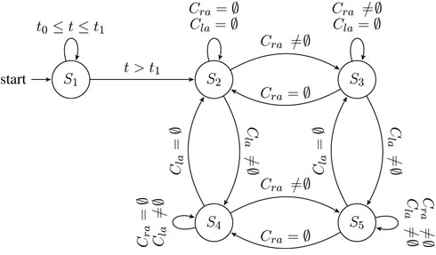
In practice, at start (t = t₀) the robot is in state S₁ in order to maintain a configuration, which is as close as possible to the initial configuration with a postural task (T ^q) that guarantees that the system is not drifting. After a predefined amount of time (t = t₁), the system switches to state S₂ by adding two tasks to the set of active tasks: a control of the forces exchanged by the left and right foot ($T_w^{\mathit{rf}}$, $T_w^{\mathit{lf}}$, respectively). The control of these forces allows for a direct control over the rate of change of the momentum as will be explained in Section 4.3. Successive transitions are triggered by the tactile sensors. If no contact is detected on the right and left arm (C_ra = ∅ and C_ra = ∅, respectively) the system remains in S₂. A transition from S₂ to S₃ is performed when the system detects a contact on the right arm (C_ra ≠ ∅): in this state, the active tasks are the same active in S₂ with the addition of the task responsible for controlling the force at the right arm contact location ($T_w^{\mathit{ra}}$). Similarly, a transition from S₂ to S₄ is performed when the system detects a contact on the left arm (C_la ≠ ∅): in this state, the active tasks are the same active in S₂ with the addition of a task responsible for controlling the force at the left arm contact location ($T_w^{\mathit{la}}$). Finally, a transition from either S₃ or S₄ to S₅ is performed whenever the robot perceives a contact so that in this new situation both arms are in contact (C_ra ≠ ∅ and C_la ≠ ∅, respectively). In S₅, both arms are used to control the interaction forces by activating the tasks $T_w^{\mathit{ra}}$ and $T_w^{\mathit{la}}$.

4.3. Task References

In this section, we discuss how to compute the task references:

$w_{\mathit{ra}}^{\ast },w_{\mathit{la}}^{\ast },w_{\mathit{rf}}^{\ast },w_{\mathit{lf}}^{\ast },{\ddot{q}}_j^{\ast }.$

to be used in the controller equation (8). Instantaneous values for forces are computed so as to follow a desired trajectory of the center of mass ($x_{\mathit{com}}^d$) and to reduce the system’s angular momentum. Instantaneous values for ${\ddot{q}}_j^{\ast }$ are chosen so as to follow a desired reference posture $q_j^d$. The latter is obtained by choosing:

${{\ddot{q}}_j}^{\ast }\left(t\right)={{\ddot{q}}_j}^d\left(t\right)-K_d^q\left({\dot{q}}_j-{{\dot{q}}_j}^d\left(t\right)\right)-K_p^q\left(q_j-{q_j}^d\left(t\right)\right),$ (12)

where $K_p^q$ and $K_d^q$ are arbitrary positive-definite matrices that take into account that in the presence of modeling errors, the acceleration imposed on the system ${\ddot{q}}_j$ might differ from the ideal one ${{\ddot{q}}_j}^{\ast }$. Instantaneous values for interaction forces are instead computed to follow a prescribed center-of-mass trajectory ($x_{\mathit{com}}^d$) and to reduce angular momentum. In order to do so, a reference value ${Ḣ}_{\mathit{com}}^{\ast }$ for the total rate of change of spatial momentum (expressed at the center of mass) is computed with a strategy similar to equation (12).

$\begin{array}{ll}\hfill {{Ḣ}_{\mathit{com}}}^{\ast }\left(t\right)& ={Ḣ}_{\mathit{com}}^d\left(t\right)-K_d^h\left(H_{\mathit{com}}-H_{\mathit{com}}^d\left(t\right)\right)-\left[\begin{array}{c}{K}_p^{\mathit{com}}\left(x_{\mathit{com}}-x_{\mathit{com}}^d\left(t\right)\right)\\ 0_{3\times 1}\end{array}\right],H_{\mathit{com}}^d=\left[\begin{array}{c}m{ẋ}_{\mathit{com}}^d\\ 0_{3\times 1}& \end{array}\right]\end{array}$ (13)

where $K_d^h$, $K_p^{\mathit{com}}$ are suitably defined gain matrices, H_com is the spatial momentum around the center of mass, x_com is the center-of-mass Cartesian position, $x_{\mathit{com}}^d$ its desired value and m is the total mass of the robot. Finally, values for $f_{\mathit{ra}}^{\ast },f_{\mathit{la}}^{\ast },f_{\mathit{rf}}^{\ast },f_{\mathit{lf}}^{\ast }$ can be computed from ${{Ḣ}_{\mathit{com}}}^{\ast }$ considering that the time derivative of the momentum equals the resultant of forces and torques if all quantities are computed with respect to the center of mass. The notation is slightly complicated due to the fact that in the different scenario states S₁, …, S₅ the meaning of f (and consequently f*) in equation (8) changes. In particular we have:

$\begin{array}{ll}\hfill S_2:f=\left[\begin{array}{c}{w}_{\mathit{rf}}\\ w_{\mathit{lf}}\end{array}\right],& S_3:f=\left[\begin{array}{c}{w}_{\mathit{ra}}\\ w_{\mathit{rf}}\\ w_{\mathit{lf}}\\ \end{array}\right],S_4:f=\left[\begin{array}{c}{w}_{\mathit{la}}\\ w_{\mathit{rf}}\\ w_{\mathit{lf}}\\ \end{array}\right],S_5:f=\left[\begin{array}{c}{w}_{\mathit{ra}}\\ w_{\mathit{la}}\\ w_{\mathit{rf}}\\ w_{\mathit{lf}}\\ \end{array}\right],\end{array}$ (14)

In the different states, the following equations on f and ${Ḣ}_{\mathit{com}}$ always hold:

$S_i:C_{S_i}f+f_g={Ḣ}_{\mathit{com}},$ (15)

where f_g is the gravitational force and where we defined $C_{S_i}$ to be the matrix that expresses the spatial forces with respect to the center of mass:

$\begin{array}{l}{C}_{S_2}=\left[{}^{com}{X}_{rf}^{*}{}^{com}{X}_{lf}^{*}\right],\\ C_{S_3}=\left[{}^{com}{X}_{ra}^{*}{}^{com}{X}_{rf}^{*}{}^{com}{X}_{lf}^{*}\right],\\ C_{S_4}=\left[{}^{com}{X}_{la}^{*}{}^{com}{X}_{rf}^{*}{}^{com}{X}_{lf}^{*}\right],\\ C_{S_5}=\left[{}^{com}{X}_{ra}^{*}{}^{com}{X}_{la}^{*}{}^{com}{X}_{rf}^{*}{}^{com}{X}_{lf}^{*}\right].\end{array}$

In literature, these equations (derived from the Newton–Euler equations) have been presented in detail by Orin et al. (2013) under the name of centroidal dynamics. The constraints (15) on f given ${Ḣ}_{\mathit{com}}$ are not sufficient to identify a unique solution. Additional constraints or requirements need to be imposed in order to properly define f * to achieve the desired momentum derivative. In order to get rid of this ambiguity, the following problem can be solved when at state S_i:

$f^{\ast }=\text{arg\hspace{0.17em}}\underset{f}{\min }\parallel f-f_0{\parallel }_W^2\text{s.t.}{C}_{S_i}f+f_g={{Ḣ}_{\mathit{com}}}^{\ast },$ (16)

where ∥ ⋅ ∥_W denotes a norm weighted with the matrix W = W^⊤ > 0. The solution of this optimization is given by:

$\begin{array}{ll}\hfill f^{\ast }& =C_{S_i}^{{†}_W}\left({{Ḣ}_{\mathit{com}}}^{\ast }-f_g\right)+\left(I-C_{S_i}^{{†}_W}{C}_{S_i}\right)f_0,C_{S_i}^{{†}_W}=W^{-1}{C}_{S_i}^{\top }{\left(C_{S_i}{W}^{-1}{C}_{S_i}^{\top }\right)}^{-1}.\end{array}$ (17)

This solution gives a set of desired forces f *, which generate the desired momentum derivative ${{Ḣ}_{\mathit{com}}}^{\ast }$. It is worth noting here that additional constraints should be imposed on the contact forces to guarantee contact stability. In particular, planar unilateral contacts should have an associated FRI lying in the contact support polygon (see Section 2.2.3) and forces should be maintained within the contact friction cones. Considering that these constraints can be approximated with a set of linear inequalities, adding them into equation (16) corresponds to transforming the problem into a quadratic program, as proposed by de Lasa et al. (2010). In the present implementation, we follow a different strategy where stability constraints are enforced by solving equation (16) with a suitable choice for the reference value f₀ and weight matrix W. To ensure that reference contact forces are stable in the sense of Section 2.2.3, we express f in a reference frame whose origin coincides with the center of the maximum circle inscribed in the contact polygon. Choosing f₀ to have a null torque component penalizes solutions whose FRI is closer to the polygon borders and this penalty monotonically increases with the distance from the center of the maximum circle. Similarly, friction cones constraints are enforced by choosing the components of f₀ to be sufficiently far from the cone borders. Assuming contact plane normals to coincide with the z-axis, cone borders distance is maximized with null x and y components. If a good choice for the z-axis force components is available, it can be used in f₀. Otherwise a viable choice is also to choose f₀ = 0 since in most realistic situations the solution f * is dominated by the component f_g, which is always non-zero.

4.4. Experimental Results

We implemented the proposed control strategy on the iCub humanoid. In a first phase, the iCub was balancing with both feet on the ground plane (coplanar flat contacts, see Figure 1). The desired center of mass position was moved left to right with a sinusoidal overimposed on its initial position x_com(t₀) along the robot transverse axis (n):

$x_{\mathit{com}}^d\left(t\right)=x_{\mathit{com}}\left(t_0\right)+n\cdot A\sin \left(\mathrm{2\pi }{f}_{r}t\right)$ (18)

with f_r = 0.15Hz and A = 0.02m (see Figure 7). The reference posture ${q_j}^d\left(t\right)$ was maintained at its initial configuration ${q_j}^d\left(t_0\right)$. As previously described the desired center-of-mass acceleration was obtained by suitably choosing the forces at the contact points (in this case at the feet) as represented in Figure 8. A video of the first phase of the experiment⁶ is available for the interested reader.

FIGURE 7

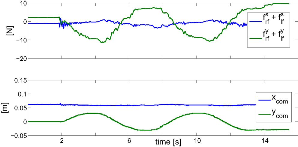
Figure 7. Results of the double-support experiment on planar contacts (left and right feet). The picture shows the time behavior of forces (top) and center of mass position (bottom) on the sagittal (blue) and transverse (green) axis. It is worth noting that forces should be proportional to center of mass accelerations and this is visible in the plot considering that accelerations are sinusoidal in counter phase with positions. Rapid variations of the contact forces at the time t ≈ 2[s], i.e., starting time, are due to the activation of the torque control.

FIGURE 8

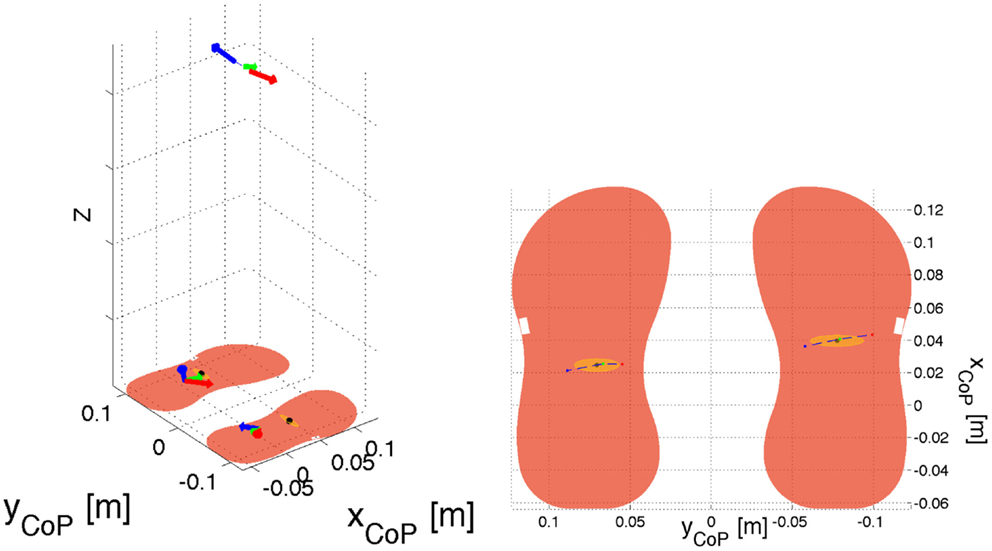
Figure 8. Results of the double-support experiment on planar contacts (left and right feet). The left picture shows in three dimensions the feet contacts, the feet center of pressures, the forces at the feet and at the center of mass during three instants: at two extrema of the sinusoid (red and blue) and in the middle of the sinusoid (green). Remarkably forces are maximum at the extrema when also accelerations are maximal. The right picture shows a close-up of the feet with the trajectory of the center of pressure, an ellipse representing a Gaussian fit of the data points and three points corresponding to the position of the centers of pressure when at the two extrema of the sinusoid (red and blue) and in the middle of the sinusoid (green).

In a second phase, the iCub was maintaining its center of mass at its initial position $x_{\mathit{com}}^d\left(t\right)\equiv x_{\mathit{com}}\left(t_0\right)$ and the joint reference posture ${q_j}^d\left(t\right)$ was chosen so as to move the arms toward a table in front of the robot. The controller equation (8) was regulated by the finite state machine described in Section 4.2. At the occurrence of contacts, forces at the arms were regulated to a predefined value f_d, which was obtained by imposing two additional constraints in solving equation (16): w_ra = w_d and w_la = w_d. The force-regulation task at the arms is shown in Figures 9 and 10, which also shows that the generation of forces at the arms does not affect the center of pressure at the feet.

FIGURE 9

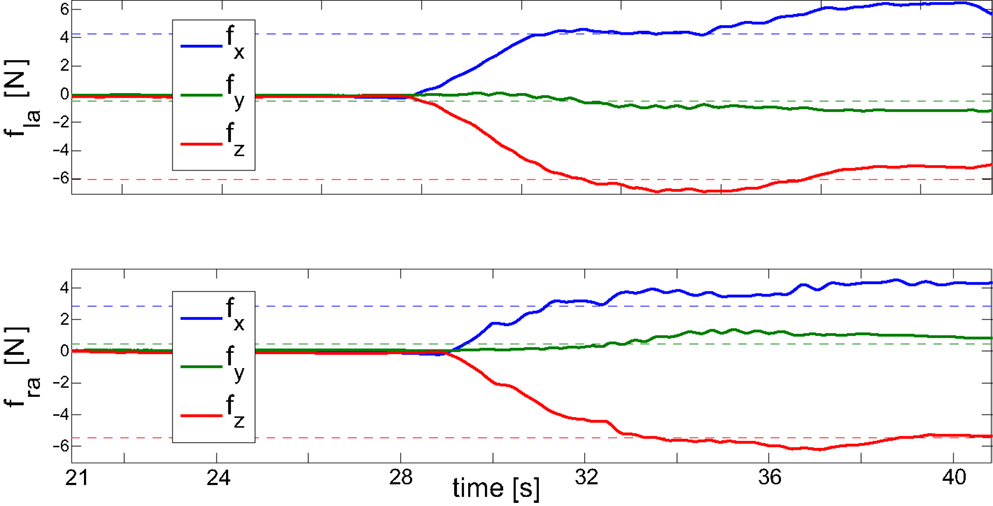
Figure 9. Results of the double-support experiment on four non-coplanar contacts (both feet and arms). The plots represent the evolution of the contact forces at the left (top) and right (bottom) arms when contact is established.

FIGURE 10

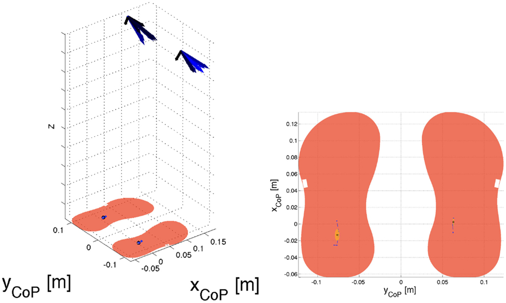
Figure 10. Results of the double-support experiment on four non-coplanar contacts (both feet and arms). The left picture gives a three-dimensional view of the foot center-of-pressure positions together with the arm contact forces. Forces are represented in a color scale that goes from black (contact establishment) to blue (steady state). The right picture gives a close-up on the foot center-of-pressure positions with an ellipse that represents the Gaussian approximation of its distribution.

5. Conclusion

The present paper addressed the problem of whole-body motion control in the presence of multiple non-coplanar and rigid contacts. The proposed solution defines a stability criterion based on the FRI of individual contacts as opposed to global stability criteria. It is argued that the FRI lying on the contact support polygon is a necessary and sufficient condition for the contacts to impose always the same motion constraints on the whole-body dynamics. These stability conditions are therefore the ones adopted in this paper in order to avoid the complications of hybrid and switching systems control. The chosen stability conditions require the capability of simultaneously measuring forces and torques (i.e., wrenches) at any possible contact location. This is not possible with conventional torque-controlled manipulators and requires whole-body distributed force and tactile sensing. These sensing capabilities are available in the iCub humanoid exploiting its whole-body distributed artificial skin and force/torque sensors. In consideration of this specific hardware, in the present paper, we discussed our approach to obtain: contact-wrench estimates, internal-torque measurement and dynamic model identification. All these components are functional to the implementation of the proposed whole-body controller with multiple non-coplanar contacts.

Conflict of Interest Statement

The authors declare that the research was conducted in the absence of any commercial or financial relationships that could be construed as a potential conflict of interest.

Acknowledgments

The authors acknowledge Ali Paikan (Istituto Italiano di Tecnologia, iCub Facility) for his contribution on the Lua bindings, Daniele Domenichelli (Istituto Italiano di Tecnologia, iCub Facility) for the codyco-superbuild support, Lorenzo Natale (Istituto Italiano di Tecnologia, iCub Facility) for the support to the YARP framework, Marco Randazzo (Istituto Italiano di Tecnologia, iCub Facility) for the implementation of torque control on the iCub humanoid, Julien Jenvrin (Istituto Italiano di Tecnologia, iCub Facility) for the technical hardware support, and Giorgio Metta for the coordination of the iCub Facility activities. Funding: This paper was supported by the FP7 EU projects CoDyCo (No. 600716 ICT 2011.2.1 Cognitive Systems and Robotics), and Koroibot (No. 611909 ICT-2013.2.1 Cognitive Systems and Robotics).

Footnotes

1. ^Normal linear motion and tangential angular motions are constrained by the unilateral contact forces; tangential linear motions and normal angular motion are constrained by friction.
2. ^The FRI and ZMP (as they have been defined) do not depend neither on the tangential forces nor on the normal moments. However, frictional constraints depend on these quantities. Therefore, no stability criteria can be formulated using only the FRI and the ZMP quantities. Within this context, it comes with no surprise that the sufficient condition for contact stability requires tangential forces and normal moments to be within the friction cones of the contact itself.
3. ^See the software library documentation http://wiki.icub.org/iCub_documentation/idyn_introduction.html
4. ^https://github.com/robotology/codyco-modules/tree/master/src/modules/motorFrictionIdentification
5. ^Both the identification equation (3) and control equation (4) are available with an open source license. See the documentation in http://wiki.icub.org/wiki/CoDyCo_Software
6. ^https://www.youtube.com/watch?v=jaTEbCsFp_M

References

Aghili, F. (2005). A unified approach for inverse and direct dynamics of constrained multibody systems based on linear projection operator: applications to control and simulation. IEEE Trans. Robot. 21, 834–849. doi: 10.1109/TRO.2005.851380

CrossRef Full Text | Google Scholar

Ayusawa, K., Venture, G., and Nakamura, Y. (2014). Identifiability and identification of inertial parameters using the underactuated base-link dynamics for legged multibody systems. Int. J. Rob. Res. 33, 446–468. doi:10.1177/0278364913495932

CrossRef Full Text | Google Scholar

Cannata, G., Maggiali, M., Metta, G., and Sandini, G. (2008). “An embedded artificial skin for humanoid robots,” in 2008 IEEE International Conference on Multisensor Fusion and Integration for Intelligent Systems (Seoul: IEEE), 434–438.

Google Scholar

de Lasa, M., Mordatch, I., and Hertzmann, A. (2010). Feature-based locomotion controllers. ACM Trans. Graph. 29, 131:1–131:10. doi:10.1016/j.neunet.2013.04.005

Pubmed Abstract | Pubmed Full Text | CrossRef Full Text | Google Scholar

Del Prete, A. (2013). Control of Contact Forces using Whole-Body Force and Tactile Sensors: Theory and Implementation on the iCub Humanoid Robot. PhD thesis, Istituto Italiano di Tecnologia, Genova.

Google Scholar

Del Prete, A., Denei, S., Natale, L., Mastrogiovanni, F., Nori, F., Cannata, G., et al. (2011). “Skin spatial calibration using force/torque measurements,” in International Conference on Intelligent Robots and Systems (San Francisco, CA: IEEE), 3694–3700.

Google Scholar

Del Prete, A., Mansard, N., Nori, F., Metta, G., and Natale, L. (2014). “Partial force control of constrained floating-base robots,” in Proceedings of 2003 IEEE/RSJ International Conference on Intelligent Robots and Systems, 2014. Chicago, IL.

Google Scholar

Del Prete, A., Natale, L., Nori, F., and Metta, G. (2012). “Contact force estimations using tactile sensors and force/torque sensors,” in Human-Robot Interaction (HRI), workshop on Advances in Tactile Sensing and Touch based Human-Robot Interaction (Boston, MA: ACM/IEEE), 0–2.

Google Scholar

Featherstone, R. (2008). Rigid Body Dynamics Algorithms. Springer.

Google Scholar

Fumagalli, M., Ivaldi, S., Randazzo, M., Natale, L., Metta, G., Sandini, G., et al. (2012). Force feedback exploiting tactile and proximal force/torque sensing. Theory and implementation on the humanoid robot iCub. Auton. Robots 33, 381–398. doi:10.1007/s10514-012-9291-2

CrossRef Full Text | Google Scholar

Goswami, A. (1999). Postural stability of biped robots and the foot-rotation indicator (fri) point. Int. J. Rob. Res. 18, 523–533. doi:10.1177/02783649922066376

CrossRef Full Text | Google Scholar

Harada, K., Kajita, S., Kaneko, K., and Hirukawa, H. (2003). “Zmp analysis for arm/leg coordination,” in Intelligent Robots and Systems, 2003. (IROS 2003). Proceedings. 2003 IEEE/RSJ International Conference on (Las Vegas: IEEE), Vol. 1, 75–81.

Google Scholar

Herzog, A., Righetti, L., Grimminger, F., Pastor, P., and Schaal, S. (2014). Balancing experiments on a torque-controlled humanoid with hierarchical inverse dynamics. doi:10.1109/IROS.2014.6942678

CrossRef Full Text | Google Scholar

Hirai, K., Hirose, M., Haikawa, Y., and Takenaka, T. (1998). “The development of honda humanoid robot,” in Robotics and Automation, 1998. Proceedings. 1998 IEEE International Conference on (Leuven: IEEE), Vol. 2, 1321–1326.

Google Scholar

Hollerbach, J., Khalil, W., and Gautier, M. (2008). “Model identification,” in Springer Handbook of Robotics, eds B. Siciliano and O. Khatib (Berlin: Springer), 321–344. Available at: http://dx.doi.org/10.1007/978-3-540-30301-5_15

Google Scholar

Huang, Q., Yokoi, K., Kajita, S., Kaneko, K., Arai, H., Koyachi, N., et al. (2001). Planning walking patterns for a biped robot. IEEE Trans. Rob. Autom. 17, 280–289. doi:10.1109/70.938385

CrossRef Full Text | Google Scholar

Hyon, S.-H., Hale, J., and Cheng, G. (2007). Full-body compliant human-humanoid interaction: balancing in the presence of unknown external forces. IEEE Trans. Robot. 23, 884–898. doi:10.1109/TRO.2007.904896

CrossRef Full Text | Google Scholar

Kajita, S., and Espiau, B. (2008). “Chapter 16 legged robots,” in Springer Handbook of Robotics, Vol. C, eds B. Siciliano and O. Khatib (Berlin: Springer), 361–389.

Google Scholar

Khatib, O. (1987). A unified approach for motion and force control of robot manipulators: the operational space formulation. IEEE J. Rob. Autom. 3, 43–53. doi:10.1109/JRA.1987.1087068

CrossRef Full Text | Google Scholar

Li, Q., Takanishi, A., and Kato, I. (1993). “Learning control for a biped walking robot with a trunk,” in Intelligent Robots and Systems ‘93, IROS ‘93. Proceedings of the 1993 IEEE/RSJ International Conference on (Yokohama: IEEE), Vol. 3, 1771–1777.

Google Scholar

Maiolino, P., Maggiali, M., Cannata, G., Metta, G., and Natale, L. (2013). A flexible and robust large scale capacitive tactile sensor for robots. IEEE Sens. J. 13, 3910–3917. doi:10.1109/JSEN.2013.2258149

CrossRef Full Text | Google Scholar

Metta, G., Natale, L., Nori, F., Sandini, G., Vernon, D., Fadiga, L., et al. (2010). The iCub humanoid robot: an open-systems platform for research in cognitive development. Neural Netw. 23, 1125–1134. doi:10.1016/j.neunet.2010.08.010

Pubmed Abstract | Pubmed Full Text | CrossRef Full Text | Google Scholar

Murray, R. M., Sastry, S. S., and Zexiang, L. (1994). A Mathematical Introduction to Robotic Manipulation, 1st Edn. Boca Raton, FL: CRC Press, Inc.

Google Scholar

Orin, D. E., Goswami, A., and Lee, S.-H. (2013). Centroidal dynamics of a humanoid robot. Auton. Robots 35, 161–176. doi:10.1007/s10514-013-9341-4

CrossRef Full Text | Google Scholar

Ott, C., Roa, M. A., and Hirzinger, G. (2011). “Posture and balance control for biped robots based on contact force optimization,” in 2011 11th IEEE-RAS International Conference on Humanoid Robots (Bled: IEEE), 26–33.

Google Scholar

Park, J. (2006). Control Strategies for Robots in Contact. PhD thesis, Stanford University, Stanford, CA.

Google Scholar

Popovic, M. B., and Herr, H. (2005). Ground reference points in legged locomotion: definitions, biological trajectories and control implications. Int. J. Rob. Res. 24, 2005. doi:10.1177/0278364905058363

CrossRef Full Text | Google Scholar

Randazzo, M., Fumagalli, M., Nori, F., Natale, L., Metta, G., and Sandini, G. (2011). “A comparison between joint level torque sensing and proximal F/T sensor torque estimation: implementation on the iCub,” in Intelligent Robots and Systems (IROS), 2011 IEEE/RSJ International Conference on (IEEE), 4161–4167. Available at: http://ieeexplore.ieee.org/xpls/abs_all.jsp?arnumber=6048660

Google Scholar

Righetti, L., Buchli, J., Mistry, M., and Schaal, S. (2011). “Control of legged robots with optimal distribution of contact forces,” in 2011 11th IEEE-RAS International Conference on Humanoid Robots (Bled: IEEE), 318–324.

Google Scholar

Sardain, P., and Bessonnet, G. (2004). Forces acting on a biped robot. Center of pressure – zero moment point. IEEE Trans. Syst. Man Cybern. A Syst. Hum. 34, 630–637. doi:10.1109/TSMCA.2004.832811

CrossRef Full Text | Google Scholar

Sentis, L. (2007). Synthesis and Control of Whole-Body Behaviors in Humanoid Systems. PhD thesis, Stanford University, Stanford, CA.

Google Scholar

Spong, M. W. (1994). “The control of underactuated mechanical systems,” in First International Conference on Mechatronics. Mexico.

Google Scholar

Stonier, D., and Kim, J.-H. (2006). “Zmp analysis for realisation of humanoid motion on complex topologies,” in Systems, Man and Cybernetics, 2006. SMC ‘06. IEEE International Conference on (Taipei: IEEE), Vol. 1, 247–252.

Google Scholar

Vukobratovic, M., and Borovac, B. (2004). Zero-moment point – thirty five years of its life. Int. J. HR 1, 157–173. doi:10.1142/S0219843604000083

CrossRef Full Text | Google Scholar

Vukobratovic, M., and Juricic, D. (1969). Contribution to the synthesis of biped gait. IEEE Trans. Biomed. Eng. 16, 1–6. doi:10.1109/TBME.1969.4502596

CrossRef Full Text | Google Scholar

Wieber, P.-B. (2002). “On the stability of walking systems,” in Proceedings of the International Workshop on Humanoid and Human Friendly Robotics. Tsukuba, Japan.

Google Scholar

Appendix

A. CoP Existence Conditions

The Poinsot theorem [see p. 65 in Murray et al. (1994)] states that every wrench applied to a rigid body is equivalent to a force applied along a fixed axis plus a torque about the same axis. In particular, let us define a wrench $\left(f_c^A,{\mathrm{\mu }}_c^A\right)$ applied at the point A. This wrench is equivalent to another wrench $\left(f_c^L,{\mathrm{\mu }}_c^L\right)$ applied at any point L on an axis l = {q′ : q′ = q + λω, ∀λ ∈ ℝ} and whose components $f_c^L$ and ${\mathrm{\mu }}_c^L$ are parallel to l, i.e., $f_c^L={\mathrm{\lambda }}_f\mathrm{\omega }$ and ${\mathrm{\mu }}_c^L={\mathrm{\lambda }}_{\mathrm{\mu }}\mathrm{\omega }$. Assuming $\parallel f_c^A\parallel \ne 0$, quantities are defined as follows:

$\mathrm{\omega }=\frac{f_c^A}{\parallel f_c^A\parallel },q=\frac{f_c^A\times {\mathrm{\mu }}_c^A}{\parallel f^A{\parallel }^2},{\mathrm{\lambda }}_f=\parallel f_c^A\parallel ,{\lambda }_{\mu }=\frac{f_c^{A^{{}^{┬}}}{\mu }_c^A}{\parallel f_c^A\parallel }.$ (A1)

The proof of the equivalence between $\left(f_c^A,{\mathrm{\mu }}_c^A\right)$ and $\left(f_c^L,{\mathrm{\mu }}_c^L\right)$ is reported by Murray et al. (1994) and therefore here omitted. In the next subsection, we prove instead that all equivalent wrenches on the Poinsot axis have minimum norm torque.

A.1. Poinsot Axis as the Geometric Locus of Minimum Torques

Besides being an equivalent wrench, the Poinsot wrench $\left(f_c^L,{\mathrm{\mu }}_c^L\right)$ has an associated minimum norm torque ${\mathrm{\mu }}_c^L$ among all equivalent wrenches. In order to prove this optimality principle, let us consider the equivalent torque ${\mathrm{\mu }}_c^Q$ at an arbitrary point Q:

${\mathrm{\mu }}_c^Q={\mathrm{\mu }}_c^L+r_{\mathit{QL}}\times f_c^L={\mathrm{\lambda }}_{\mathrm{\mu }}\mathrm{\omega }+r_{\mathit{QL}}\times {\mathrm{\lambda }}_f\mathrm{\omega },$ (A2)

being r_QL the vector connecting L to Q. Applying the norm to the above equation and observing that the sum is an orthogonal decomposition, we obtain:

$\parallel {\mathrm{\mu }}_c^Q\parallel =\parallel {\mathrm{\lambda }}_{\mathrm{\mu }}\mathrm{\omega }\parallel +\parallel r_{\mathit{QL}}\times {\mathrm{\lambda }}_f\mathrm{\omega }\parallel \ge \parallel {\mathrm{\lambda }}_{\mathrm{\mu }}\mathrm{\omega }\parallel =\parallel {\mathrm{\mu }}_c^L\parallel .$ (A3)

Therefore, $\Vert {\mu }_c^Q\Vert \ge \Vert {\mu }_c^L\Vert$ and the equality holds if and only if r_QL is parallel to ω, i.e., when Q lies on the Poinsot axis defined as:

$\left\{q\prime :q\prime =\frac{f_c^A\times {\mathrm{\mu }}_c^A}{\parallel \mathit{fA}\parallel 2}+\mathrm{\lambda }\frac{f_c^A}{\parallel f_c^A\parallel },\forall \mathrm{\lambda }\in \mathbb{R}\right\}.$ (A4)

On the Poinsot axis, the torque norm is minimal and equals:

$\Vert {\mu }_c^{min}\Vert =\frac{f_c^{A{}^{┬}}{\mu }_c^A}{\Vert f_c^A\Vert }.$ (A5)

A.2. CoP Existence and Poinsot Axis

Given a rigid body subject to a field of pressures, the center of pressure (CoP) is an application point where the equivalent torque (due to the field of pressure) is null. Being the Poinsot axis, the geometric locus of minimum torques, it is evident that a CoP can be defined if and only if $\Vert {\mu }_c^{min}\Vert =0$, or equivalently if and only if f_c and μ_c are orthogonal. When this is the case, the CoP is not uniquely defined and the geometric locus of valid CoP corresponds to the Poinsot axis (22).

B. Counterexample on the Global CoP as a Contact Stability Criteria

In this section, we provide a counterexample to show that the condition on GCoP (global center of pressure) to lie in the contacts convex hull is not sufficient to guarantee the stability of individual contacts. Consider the simple system represented in Figure A1. For certain values of the torques at the joints the global stability criteria are met (i.e., the GCoP lies in the convex hull of contacts) but individual contacts are unstable (i.e., the FRI of each contact lies outside the contact area). Given the unilateral nature of the contacts acting on the system, its solution is non-trivial and requires to make hypotheses on whether or contacts break or persist as clearly explained by Featherstone (2008) in chapter eleven of his book. In the specific case of Figure A1, however, it would be sufficient to just provide that particular situation in which torques at the joints force contacts to break while maintaining the GCoP within the contact support polygon. This specific situation is presented in B.3. For sake of clarity, we start with discussing the case in which contacts persist. This case just helps in understanding the proposed counterexample.

FIGURE A1

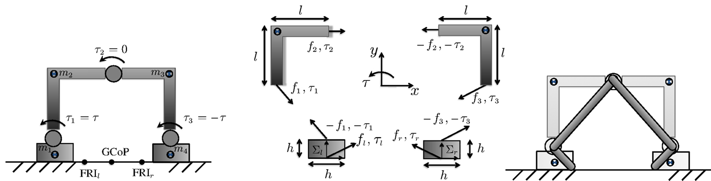
Figure A1. The image shows the example of an articulated rigid body with two links in contact with the ground. Left figure. The system is composed of four rigid bodies. The centers of mass associated to the rigid bodies are indicated with a check board circle. Three rotational joints have associated torques τ₁, τ₂, and τ₃. Central figure. The sketch shows the convention and the geometric dimension used in the computations. The contact interaction forces are indicated with f_r, f_l ∈ ℝ², τ_r, τ_l ∈ ℝ; the internal constraint forces are indicated with f₁, f₂, f₃ ∈ ℝ². Right figure. The linkage that describes the system kinematic constraints when assuming that the left foot is pivoting around its right edge and the right foot around its left edge.

B.1. ZMP Computation

In this section, we provide explicit computation for the zero tipping moment point associated to a wrench w_c = (f_c, μ_c) applied at a generic point P. It is worth stressing once more that the zero tipping moment point is by definition the ZMP, the latter name being misleading. For sake of simpler notation, let the contact plane coincide with the x-y plane. Given the contact wrench w_c = (f_c, μ_c) at a generic point P = [P_x, P_y, 0] of the contact plane, the equivalent torque ${\mathrm{\mu }}_c^{\prime }$ at $P\prime =\left[P_x^{\prime },P_y^{\prime },0\right]$ is given by:

${\mathrm{\mu }}_c^{\prime }=-r_{P{P}^{\prime }}\times f_c+{\mathrm{\mu }}_c=\left[\begin{array}{c}\hfill {\mathrm{\mu }}_c^x-r_{P{P}^{\prime }}^y{f}_c^z\hfill \\ \hfill {\mathrm{\mu }}_c^y+r_{P{P}^{\prime }}^x{f}_c^z\hfill \\ \hfill {\mathrm{\mu }}_c^z-r_{P{P}^{\prime }}^x{f}_c^y+r_{P{P}^{\prime }}^y{f}_c^x\hfill \\ \hfill \hfill \end{array}\right]$ (A6)

where r_PP′ = P′ − P. At a particular point P′the tipping moments along the x and y axes equal zero. This point corresponds to the zero tipping moment associated to w_c = (f_c, μ_c) and equals:

$r_{\text{ZMP}}^x=-\frac{{\mathrm{\mu }}_c^y}{f_c^z},r_{\text{ZMP}}^y=\frac{{\mathrm{\mu }}_c^x}{f_c^z}.$ (A7)

Assuming that the contact wrench w_c = (f_c, μ_c) is the resultant of a field of pressures p_c on the surface S, we have:

$f_c^z={\int }_S{p}_c\mathit{dS},{\mathrm{\mu }}_c^x={\int }_{S}y{p}_c\mathit{dS},{\mathrm{\mu }}_c^y={\int }_S-x{p}_c\mathit{dS}.$ (A8)

Therefore, we have:

$r_{\text{ZMP}}^x={\int }_{S}x\mathrm{\alpha }\mathit{dS},r_{\text{ZMP}}^y={\int }_{S}y\mathrm{\alpha }\mathit{dS},\mathrm{\alpha }=\frac{p_c}{{\int }_S{p}_c\mathit{dS}},$ (A9)

where in case of unilateral contacts (p_c ≥ 0) it results evident that the ZMP is the convex combination of points in S and as such it belongs to the convex hull of S.

B.2. Equilibrium Configurations

In the following paragraphs, we study equilibrium configurations for the system in Figure A1. Let us first consider the case in which both contacts are active. The idea is to find conditions on the applied torques to guarantee that the system is in dynamic equilibrium (i.e., null accelerations) and contacts persist. The planar Newton–Euler equilibrium equations for each of the 4 rigid bodies composing the system give 12 equations. Interaction (f_r, f_l ∈ ℝ², τ_r, τ_l ∈ ℝ) and internal (f₁, f₂, f₃ ∈ ℝ²) forces and torques give twelve unknowns that can be uniquely solved for any choice of the joint torques τ₁, τ₂, τ₃. To simplify the notation and to obtain a symmetric solution we assume τ₁ = τ, τ₂ = 0, τ₁ = − τ. Solving the associated equations gives the following solution for the contact forces:

$f_r=\left[\begin{array}{c}\hfill \mathrm{\tau }∕l\hfill \\ \hfill \left(m_3+m_4\right)g\hfill \end{array}\right],f_l=\left[\begin{array}{c}\hfill -\mathrm{\tau }∕l\hfill \\ \hfill \left(m_1+m_2\right)g\hfill \end{array}\right],$ (A10a)

${\mathrm{\tau }}_r=-\mathrm{\tau }\left(1+\frac{h}{l}\right),{\mathrm{\tau }}_l=\mathrm{\tau }\left(1+\frac{h}{l}\right),$ (A10b)

and internal forces:

$\begin{array}{l}\hfill f_1=\left[\begin{array}{c}\mathrm{\tau }∕l\\ m_{2}g\end{array}\right],f_2=\left[\begin{array}{c}\mathrm{\tau }∕l\\ 0\end{array}\right],f_3=\left[\begin{array}{c}-\mathrm{\tau }∕l\\ m_{3}g\end{array}\right].\end{array}$ (11)

Assuming for the sake of simpler notation m₁ + m₂ = m₃ + m₄ = m_tot/2, (28) gives the following expressions for the local right and left foot FRI¹ (expressed in the associated reference frames Σ_r and Σ_l, respectively):

$\begin{array}{lll}\hfill {\text{FRI}}_r=\left[\begin{array}{c}-\mathrm{\tau }\frac{h+l}{\mathit{mlg}∕2}\\ 0\end{array}\right],{\text{FRI}}_l=\left[\begin{array}{c}\mathrm{\tau }\frac{h+l}{\mathit{mlg}∕2}\\ 0\end{array}\right].& & \hfill \end{array}$

The global center of pressure (GCoP) can be computed by representing f_r, f_l, τ_r, and τ_l in a common reference frame to obtain the total force and torque f_tot-τ_tot. Using a reference frame in the middle of the two contacts we have:

$\begin{array}{l}\hfill {\mathrm{\tau }}_{\mathit{tot}}^l={\mathrm{\tau }}_r+l{f}_r^y+{\mathrm{\tau }}_l-l{f}_l^y=0,f_{\mathit{tot}}^l=\left[\begin{array}{c}0\\ \mathit{mg}\end{array}\right],\end{array}$

and therefore GCoP = [0, 0]^T. As expected by the system symmetry, the global center of pressure is always in the middle of the two contacts regardless of the value given to τ. Instead, the local contacts rotation indicators FRI_r and FRI_l linearly depend on τ and, for a given contact geometry, it is always possible to find a τ, which brings them outside the contact areas. As an example, we can assume that the surfaces in contact have width 2h (twice the foot height) and, for sake of simpler notation h = l/2. With this simplification the FRI is within the support polygon of each contact if and only if:

$\begin{array}{lll}\hfill -\frac{\mathit{mgl}}{6}\le \mathrm{\tau }\le \frac{\mathit{mgl}}{6}.& & \hfill \end{array}$

If τ ≥ mgl/6, the left foot rotation indicator FRI_l is on the right of the left foot support polygon. Similarly, FRI_r is on the left of the right foot support polygon. In practice, recalling the results presented in Section 2.2, this fact implies that the computed f_r, τ_r, f_l, τ_l for the system equilibrium cannot be generated by a unilateral contact of the given geometry. In a sense, the equilibrium assumption is wrong and we need to redo computations with a different assumption. In the following, we assume that the left foot is rotating with respect to its right edge and that the right foot is rotating with respect to its left edge. We then check that the solution found is feasible in terms of contact forces.

B.3. Inward Feet Rotation Configurations

In this section, we make the hypothesis that contact constraints force the left foot to rotate around its right edge and the right foot around its left edge. In this specific case, the torques at the (point wise) contacts is identically null. With respect to the previous situation we therefore have two unknowns less. Additional unknowns come from the fact that we are no longer assuming accelerations to be identically null since the system is no longer assumed at equilibrium. These additional unknowns can be expressed as a function of only two unknowns (e.g., the left and right foot tipping accelerations). This results by taking into consideration the kinematic constraints in the system, as represented in the left hand side of Figure A1. Therefore, with respect to the equilibrium case we removed two unknowns (the torques at the contacts) and inserted other two (the foot angular acceleration at the tipping point). As a result, the Newton–Euler system of equations is still solvable. Deriving the solution is out of the scope of the present paper and therefore omitted. The interested reader can have a look at the computations, which are available in Matlab². We report here the values of some important variables such as the right and left foot acceleration (denoted ${\ddot{q}}_r$ and ${\ddot{q}}_l$):

$\begin{array}{lll}\hfill {\ddot{q}}_r=k\left(\mathrm{6\tau }-\mathit{mgl}\right),{\ddot{q}}_l=-k\left(\mathrm{6\tau }-\mathit{mgl}\right).& & \hfill \end{array}$

for some positive scalar k > 0 which depends only on the system geometric and dynamic parameters. By convention positive accelerations correspond to counter clock wise rotations. As soon as the right foot FRI starts moving away from its left edge (τ > mgl/6) the right foot starts counter clock wise rotating. Similarly, when the left foot FRI moves away from its right edge (again, τ > mgl/6) the left foot starts clock wise rotating. The left foot FRI can be computed as well. Given that the foot is not in equilibrium, FRI_l is computed using f₁ and τ₁ reprojected on the planar contact surface. Similar considerations hold for FRI_r. The position of the left and right feet rotation indicators with respect to the pivoting point is given by:

$\begin{array}{lll}\hfill {\text{FRI}}_l=\frac{\mathrm{6\tau }-\mathit{mgl}}{k_1+k_2\mathrm{\tau }},{\text{FRI}}_r=-\frac{\mathrm{6\tau }-\mathit{mgl}}{k_1+k_2\mathrm{\tau }}& & \hfill \end{array}$

where k₁ and k₂ are positive scalars which again depend only on the system geometric and dynamic parameters. As expected FRI_r and FRI_l coincide with the pivoting point (the edge of the support polygon) when τ = mgl/6 and move away from the support polygon when τ > mgl/6. The vertical forces at the contact have the following expressions:

$f_l^y=k_3\mathrm{\tau }+k_4,f_r^y=k_3\mathrm{\tau }+k_4$

for positive constants k₃ and k₄. Contact forces are therefore positive as expected given the unilaterally of the contact. Finally, given the symmetry of the problem, the GCoP is constantly at the center of symmetry of the system and therefore within the contact support polygon. Therefore, when τ > mgl/6 the system starts rotating feet at their edges (contacts are broken) even if the global center of pressure is within the contact convex hull. This is therefore the counterexample we were looking for.

Footnotes

1. ^Using the FRI definition and assuming the contact plane to be y = 0, a force f and a torque τ have an associated FRI with x-coordinate given by FRIx = τ/f y.
2. ^https://github.com/iron76/wholeBodyCounterExample