Analyzing the effects of instance features and algorithm parameters for max–min ant system and the traveling salesperson problem

1. Introduction

Ant colony optimization (ACO) (Dorigo and Stützle, 2004) has become very popular in recent years to solve a wide range of hard combinatorial optimization problems. Throughout the history of heuristic optimization, attempts have been made to analyze ACO algorithm performance theoretically (Stützle and Dorigo, 2002; Kötzing et al., 2011, 2012) and experimentally (Pellegrini et al., 2006; Stützle et al., 2012). However, much less work has been done toward the goal of explaining the impact of problem instance structure and algorithm parameters on performance.

The traveling salesperson problem (TSP) is one of the most famous NP-hard combinatorial optimization problems. Given a set of n cities {1, …, n} and a distance matrix d = (d_ij), 1 ≤ i, j ≤ n, the goal is to compute a tour of minimal length that visits each city exactly once and returns to the origin. The problem is proved to be NP hard as a result of the proof for the Hamiltonian cycle problem by Karp (2010). It has many real world applications in logistics, scheduling, and manufacturing. These include classical applications (Lenstra and Rinnooy Kan, 1975), such as vehicle routing (Applegate et al., 2002), order picking in warehouses (Ratliff and Rosenthal, 1983), computer wiring (Lenstra and Rinnooy Kan, 1975), overhauling of gas turbine engines (Plante et al., 1987), drilling of printed circuit boards (Grtschel et al., 1991), and X-ray crystallography (Bland and Shallcross, 1989), as well as more recent applications, such as genome sequencing (Agarwala et al., 2000), spacecraft interferometry (Bailey et al., 2000), and vehicle navigator systems.

In early research, problem hardness analysis of TSP is based on only a few features considering edge cost distribution (Fischer et al., 2005; Ridge and Kudenko, 2008). There, algorithms are typically run on predetermined instances, and runtime or accuracy is measured. Later on, more sophisticated methods (Smith-Miles et al., 2010; Mersmann et al., 2013; Nallaperuma et al., 2013a) are introduced, for instance, generation. However, a comprehensive analysis of the effects of TSP instance features and algorithm parameters and their relationship on ACO performance has not been conducted so far.

We study the potential of feature-based characterization to be used in automatic algorithm configuration for ACO and consider the well-known Max–Min Ant System (Stützle and Hoos, 2000) for the TSP. One important question in the configuration of ACO algorithms is to what extent pheromone values, heuristic information, and population size should influence the behavior of the algorithm – the importance of these components is determined by the parameters α, ρ (for pheromone values), β (for heuristic information), and n (number of ants). We first investigate statistical features of evolved (hard, easy, and in-between) instances from Nallaperuma et al. (2013b) and their impact on the appropriate choice of these parameters. Based on this, we build a prediction model in order to predict the right choice, for instance, of TSPLIB (Reinelt, 1991). The potential strength of the prediction model relies on the wide range and on the diversity of the evolved instances, and on the expressiveness of selected structural features of problem hardness for algorithm instances. Our experimental investigations show that the considered features and evolved instances are well suited to predict an appropriate choice for setting the parameters, such as α, β, ρ, and n, of MMAS.

This article is a significant extension the conference version (Nallaperuma et al., 2014). We expand the feature-based analysis of MMAS on the TSP that is originally conducted for the two parameters, α and β (Nallaperuma et al., 2014), for another two significant MMAS parameters, namely, ρ the pheromone update strength and n the number of ants. Furthermore, we extend the preliminary prediction model presented in the conference version (Nallaperuma et al., 2014).

The outline of the paper is as follows. In Section 2, we introduce the algorithm and the framework of our investigations. In Section 3, we report on easy and hard instances for different parameter combinations and carry out a feature-based analysis first for α and β. In Section 4, the analysis is extended to ρ and n. Subsequently, we use these insights to predict parameters for given instances from TSPLIB in Section 5, and we finish with some concluding remarks.

2. Preliminaries

In this section, we discuss the basic ideas about TSP and ACO, and the preliminary work on hard and easy instance generation.

2.1. Traveling Salesperson Problem

Generally, an instance of the TSP consists of a set V = {ν₁, …, ν_n} of n vertices (depending on the context, synonymously referred to as points) and a distance function d: V × V → R ≥ 0 that associates with each pair ν_i, ν_j. Similarly, in a graph-based representation, this can be represented by a complete graph G(V, E). The goal is to find a Hamiltonian cycle of minimum length. A Hamiltonian cycle is a cycle that visits each city exactly once and returns to the origin. We also use the term tour to denote a Hamiltonian cycle. A candidate solution of the TSP is a permutation x: V → V. We sometimes associate a permutation x with its linear form, which is simply the length-n sequence [x(1), x(2), …, x(n)]. The Hamiltonian cycle in G induced by a permutation x is the set of n edges

$\begin{array}{lll}\hfill C\left(x\right)=\left\{\left\{x\left(1\right),x\left(2\right)\right\},\left\{x\left(2\right),x\left(3\right)\right\},\dots ,\left\{x\left(n-1\right),x\left(n\right)\right\},\left\{x\left(n\right),x\left(1\right)\right\}\right\}.& & \hfill \end{array}$

The optimization problem is to find a permutation x, which minimizes the fitness function

$f\left(x\right)={\displaystyle \sum _{\{u,v\}\in C\left(x\right)}d\left(u,v\right)}.$ (1)

A TSP instance is considered to be metric if its distance function is in metric space. Metric space satisfies reflexivity, symmetry, and triangle inequality conditions. A pair (V, d) of a set V and a function d: V × V → R ≥ 0 is called a metric space if for all ν_i, ν_j, ν_k ∈ V the following properties are satisfied:

• d(ν_i, ν_j) = 0 if and only if ν_i = ν_j,

• d(ν_i, ν_j) = d(ν_j, ν_i)

• d(ν_i, ν_k) ≤ d(ν_i, ν_j) + d(ν_j, ν_k).

We consider the n cities are given by points ν_i(x_i, y_i), 1 ≤ i ≤ n, in the plane. For a distance metric L_p, the distance of two points ν_i = (x_i, y_i) and ν_j = (x_i, y_i) is

$d_p\left(v_i,v_j\right)={\left({{|x}_i-x_j|}^p+{{|y}_i-y_j|}^p\right)}^{1∕p}.$

Within this research, we study the Euclidean TSP, which is a prominent case of the metric TSP having the distance metric Euclidean (L₂). The first and naive approach to solve the TSP is based on brute force search. This would take O(n!) time to solve the TSP. Later on, various improvements on this runtime have been made using different approaches, such as branch and cut (Applegate et al., 2002) the iterative heuristic by Lin and Kernighan (1973) and ant colony optimization (ACO) (Dorigo and Stützle, 2004). For a general discussion on the state of art of the TSP, we refer the interested reader to the text book by Applegate et al. (2007).

2.2. Ant Colony Optimization

Ant colony optimization (ACO) is a recent popular bio-inspired approach (Dorigo and Stützle, 2004). ACO is inspired by the foraging behavior of ants. The general structure of ACO algorithms is outlined in Algorithm 1. Individual solution tours are constructed (see Algorithm 2) at each iteration by a set of artificial ants.

ALGORITHM 1

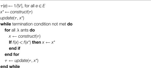
Algorithm 1. Outline of Ant Colony Optimization (ACO).

ALGORITHM 2

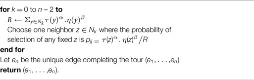
Algorithm 2. Construct.

These tours are built by visiting each node in a tour sequentially according to a probabilistic formula that takes specific heuristic information and pheromone trails into account. This probabilistic formula, called the random proportional rule, specifies a transition probability p_ij that an ant currently visiting node i selects node j next in its tour. This probability is defined as

$p_{\mathit{ij}}=\frac{{\left[{\mathrm{\tau }}_{\mathit{ij}}\right]}^{\mathrm{\alpha }}{\left[{\mathrm{\eta }}_{\mathit{ij}}\right]}^{\mathrm{\beta }}}{\left({\sum }_{h\in N_k}{\left[{\mathrm{\tau }}_{\mathit{ih}}\right]}^{\mathrm{\alpha }}{\left[{\mathrm{\eta }}_{\mathit{ih}}\right]}^{\mathrm{\beta }}\right)}$ (2)

Here, N_k represents the set of nodes that have not yet been visited by ant k, [τ_ih] and [η_ih] represent the pheromone trail intensity and the heuristic information, respectively. Hence, the parameters, α and β, accordingly adjust the effects of the pheromone and the heuristic information on the selection decision.

As above-mentioned, our study is focused on a popular ACO variant called Max–Min Ant System (MMAS) (Stützle and Hoos, 2000). In the Max–Min Ant System, the pheromone update is performed after the tour construction of ants according to ${\tau }_{ij}=\left(1-\rho \right){\tau }_{ij}+\Delta {\tau }_{ij}^b$, where ρ denotes the evaporation rate and

$\mathrm{\Delta }{\mathrm{\tau }}_{\mathit{ij}}^b=\left\{\begin{array}{cc}1∕C_b\hfill & \text{if}\left(i,j\right)\text{belongs to the best-so-far tour};\hfill \\ 0\hfill & \text{otherwise}.\hfill \end{array}\right.$

Here, C_b is the cost of the best-so-far tour (the iteration-best tour is also sometimes used). Additionally, local search can be applied upon these constructed solutions to improve them further. Pheromone trails in MMAS are bounded between maximum (τ_max) and minimum (τ_min) limits. A detailed description of this algorithm on the TSP can be found in the textbook on ACO (Dorigo and Stützle, 2004).

2.3. Problem Hardness Analysis

Throughout the history of heuristic optimization, attempts have been made to analyze ACO algorithm performance theoretically (Stützle and Dorigo, 2002; Kötzing et al., 2011, 2012) and experimentally (Pellegrini et al., 2006; Stützle et al., 2012). However, much less work has been done toward the goal of explaining the impact of the problem instance structure and the algorithm parameters on performance.

Previously, problem hardness analysis of TSP is based on only a few features considering edge cost distribution (Fischer et al., 2005; Ridge and Kudenko, 2008). There, algorithms are typically run on predetermined instances, and runtime or accuracy is measured. Later on, more sophisticated methods are introduced for the instance generation. One of the commonly used approaches is the use of an evolutionary algorithm to evolve random sets of instances into sets of instances of extreme difficulties. Recent research of TSP hardness analysis (Smith-Miles et al., 2010; Mersmann et al., 2013; Nallaperuma et al., 2013a) is based on this method, and the investigated problem features are more enriched including several feature groups describing TSP instances in terms of distances, angles, nearest neighbors, convex hull, cluster, centroid, minimum spanning tree, etc.

In contrast to the experimental approach, Pellegrini et al. (2006) proposed an analytical approach to examine parameters and their impact on the speed of convergence. They have considered the number of ants, the pheromone evaporation rate, and the exponents α and β of the pheromone trails, and the heuristic information in the random proportionate rule. Some theoretical reasoning was done in order to derive more general knowledge on the impact of parameters, and arguments were supported by several experiments. These included running algorithm instances with varying parameter settings on a set of instances. However, the authors considered only the runtime, thus, neglecting the actual resulting solution quality. Hence, the impact of the parameters on the optimality of the solution is missing in that work.

In current literature, a comprehensive analysis of ACO problem features has not been conducted. Therefore, we believe conducting a comprehensive analysis of problem hardness features based on the diverse feature set introduced by Smith-Miles and Lopes (2012) and expanded by Mersmann et al. (2013) will contribute to ACO research greatly in algorithm design and parameter selection. Next, we will discuss existing parameter selection approaches in ACO and the potential of hardness analysis to be used in parameter selection.

2.4. Parameter Prediction

The study by Stützle et al. (2012) provides an overview of existing parameter prediction/tuning approaches for ACO in two major directions: (1) parameter choosing before running the algorithm (offline tuning) and (2) adaptation during runtime (online tuning). Offline tuning is conventionally done using trial and error methods, which is error prone, and even any good results achieved cannot necessarily be reproduced. Later on, some studies have been done using an EA and local search for offline parameter tuning (Pilat and White, 2002). For example, the irace package (López-Ibáñez et al., 2011) is an automatic algorithm configuration package based on the iterative racing and ranking. Some recent work in multi-objective ant algorithms (López-Ibáñez and Stützle, 2012) used these techniques, claiming to outperform conventional offline tuning methods.

One of the sub-categories of online tuning is the prescheduled parameter adaptation, where parameter values are determined by a formula before the algorithm is run (Stützle et al., 2012). Alternatively, in adaptive parameter tuning, the parameter modification scheme is defined as a function of some statistics derived from the algorithm behavior. Similarly, in search-based adaptation schemes, parameter tuning is done by an additional evolutionary or local search algorithm during runtime.

The comparison of the two techniques (Pellegrini et al., 2010) on MMAS and TSP claims offline tuning outperformed online tuning. Nevertheless, current offline parameter configuration techniques are time consuming and use a lot of computing power, as they need to run iteratively on the instances we need to tune on. So far, to the best to our knowledge, none of these approaches have taken the problem instance structure into consideration when setting algorithm parameters.

Therefore, we believe that we can provide insights into more enhanced algorithm configuration through our problem structure analysis. In contrast to above approaches, we propose to re-use the results of hardness analysis to feed a learning system, which is capable of predicting the best parameter configuration for a new instance. Such a system could instantly propose the best parameter setting for a given input instance having its hardness features calculated. The recent studies of Hutter et al. (2013) and Muñoz et al. (2012) provide ideas on the possibility of more effective automatic algorithm configuration using both problem instance features and parameters. We find this insightful with our approach on ACO to use our resultant instance features on problem hardness analysis for parameter prediction models. However, none of the current parameter prediction approaches have considered the possibility of using an evolved set of instances.

2.5. Easy and Hard Instance Generation

To evolve easy and hard instances for the ant algorithms, we use the evolutionary algorithm approach previously studied on 2-opt (Mersmann et al., 2013) and approximation algorithms (Nallaperuma et al., 2013a) for the TSP. The only difference in the instance generation process here is that we consider several algorithm instances with different parameter settings instead of a single algorithm.

The approximation ratio α_A(I) of an algorithm A for a given instance I is defined as

${\mathrm{\alpha }}_A\left(I\right)=A\left(I\right)∕\mathit{OPT}\left(I\right)$

where A(I) is the tour length produced by algorithm A for the given instance I, and OPT(I) is the value of an optimal solution of I. OPT(I) is obtained by using the exact TSP solver Concorde (Applegate et al., 2002).

3. Features of Hard and Easy Instances for α and β

3.1. Experimental Setup

For each ACO algorithm instance with a specific parameter setting of α and β, a set of 100 random TSP instances is generated in the two-dimensional unit square [0,1]² and placed on a discretized grid. The evolutionary algorithm runs on them for 5000 generations in order to generate a set of hard and a set of easy instances. Each ACO execution is limited to 2 s. The choice of the time budget is based on experimental observation that this time budget was sufficient for ACO to converge for the considered instance sizes. In each iteration, the ACO algorithm is run once on a single instance, and then, the approximation ratio is calculated. In separate runs, either a higher approximation ratio is favored to generate hard instances, or a lower ratio is favored to generate easy instances. This process is repeated, for instance, of sizes 25, 50, 100, and 200 with the goal of generating easy and hard instances. The instance generation is performed on an Unix cluster with 48 nodes where each node has 48 cores (four AMD 6238 12-core 2.6 Ghz CPUs) and 128 GB memory (2.7 GB per core).

In this article, we consider 47 instance features including distances of edge cost distribution, angles between neighbors, nearest neighbor statistics, mode, cluster, and centroid features, as well as features representing minimum spanning tree heuristics and of the convex hull. A detailed description of these features can be found in the article by Nallaperuma et al. (2013a).

The algorithm parameters considered in this section are the most popular and critical ones in any ACO algorithm, namely, the exponents α and β, which represent the influence of the pheromone trails and heuristic information, respectively. We consider three parameter settings for our analysis: setting 1 represents default parameters (α = 1, β = 2), and settings 2 and 3 represent extreme settings with highest and lowest values in a reasonable range (α = 0, β = 4 and α = 4, β = 0). The general idea behind the choice is that we have to isolate the conditions to investigate the effect, which is usually considered in traditional scientific experiments. The rest of the parameters are set in their default values (ρ = 0.2, ants = 20) as in the original MMAS implementation by Stützle (2012).

3.2. Feature Analysis

Across all experiments, the distances between cities on the optimal tour are more uniformly distributed in the hard instances than in the easy ones. Examples of the hard and the easy instances are shown in Figure 1. The approximation ratio is very close to 1 for all generated easy instances, whereas for the hard instances it is higher, ranging from 1.04 to 1.29.

FIGURE 1

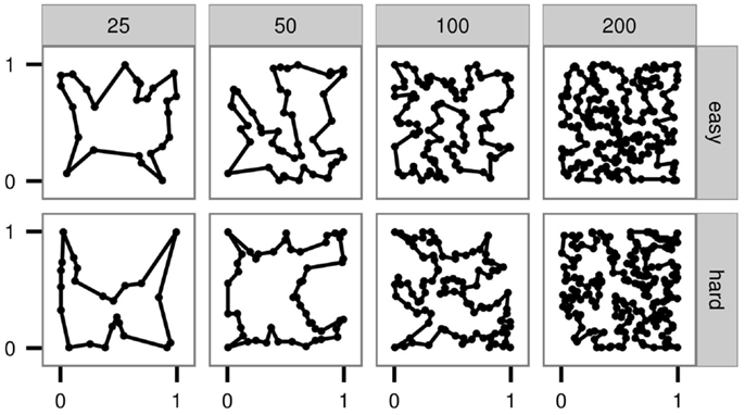
Figure 1. Instance examples.

Our experimental results for the MMAS with the three considered parameter settings show the following. For the first and the second parameter settings, the SD of angles of the easy instances are significantly smaller than the values of the hard instances, as shown in Figure 2. These values for both the hard and the easy instances slightly decrease with increasing instance size. With increasing instance size, these values change differently for easy and hard instances. Interestingly, this structural difference is even obvious to human observers who perceive different “shapes” for easy/hard and smaller/larger instances. It can be observed that the shapes of the smaller instances structurally differ from the respective shapes of larger instances. Generally, the results of the second parameter setting are similar to those of the first setting. For example, the SD of angles to the next two nearest neighbors follows a similar pattern for the second parameter combination (α = 0, β = 4), as shown in Figure 2. In contrast to the patterns of the first two parameter settings, the third combination (α = 4, β = 0) shows an increasing pattern of SD values (with increasing instance size), whereas these values follow a decreasing pattern in the case of the second setting (see Figure 2). We have further performed Wilcoxon signed rank tests (Wilcoxon, 1945) to compare the hard and easy instances based on these features for the considered parameter settings. The results of the statistical tests as shown in Table 1 verify the visual observations in above boxplots shown in Figure 2. We form the alternative hypothesis as easy instances have higher feature values than hard instances for test 1 and the converse for test 2. The statistically significant results are indicated by small p-values (<0.002). Results of test 1 support our claim that hard instances have higher feature values than easy instances for the parameter settings 1 and 2. Similarly, the converse is supported from test 2 for the parameter setting 3. And, we reject the hull hypothesis that they are not different.

FIGURE 2

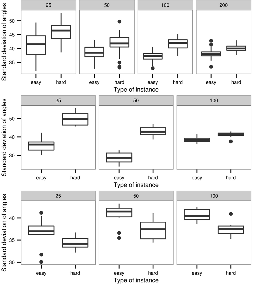
Figure 2. Boxplots of the SDs of the angles between adjacent cities on the optimal tour for parameter setting 1 (α = 1, β = 2) in top, 2 (α = 0, β = 4) in middle and setting 3 (α = 4, β = 0) in bottom.

TABLE 1

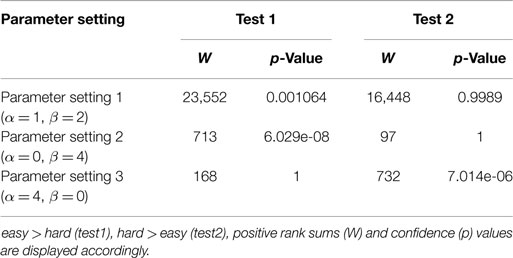
Table 1. Results of Wilcoxon signed rank tests for the SD of angles of the easy and hard instances for the three parameter settings.

The boxplots discussed previously exhibit the individual capabilities of problem features to express the problem hardness. However, not all the features have the capability to express the problem hardness individually. Nevertheless, some features in collaboration can classify hard and easy problem instances into separate clusters (see Figure 3). For all studied parameter settings, such feature combinations can be found. This implies that problem features can be used to determine the hardness or easiness of problem instances for ACO algorithms instantiated with different parameter settings. Interestingly, the type of the best classifying feature combinations and their strengths were different for the three parameter settings. For example, as shown in Figure 3, the centroid and the convex hull features are the best to classify hard and easy instances for parameter setting 2 (α = 0, β = 4), where as the distance and the angle features are dominant in the classification for parameter setting 3 (α = 4, β = 0). These results highlight the different impacts of heuristic information (on centroid and convex hull features) and pheromone information (on distance and angle features) in determining the hardness and easiness of problem instance for ACO (i.e., for MMAS in particular).

FIGURE 3

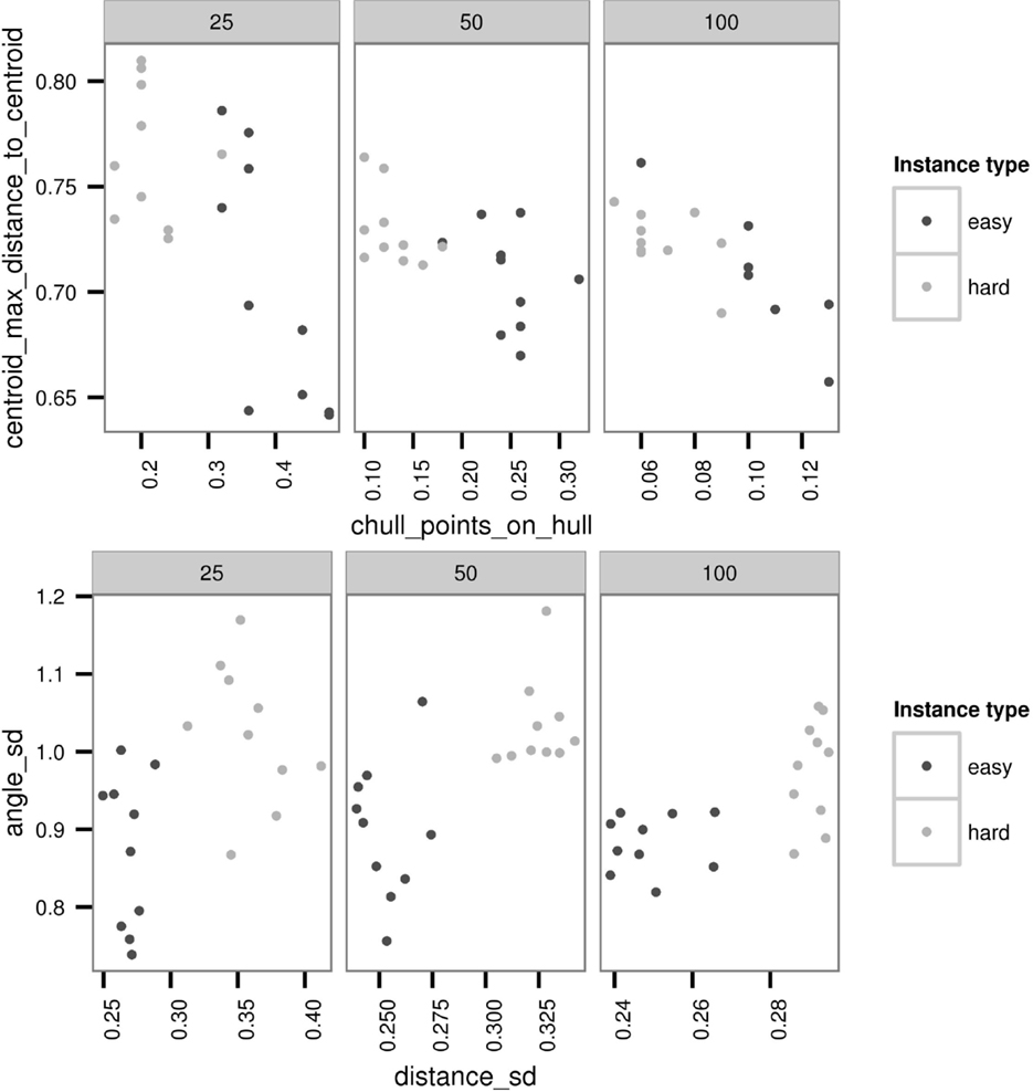
Figure 3. Hard and easy classification with two exemplary feature combinations maximum distance to centroid and the number of points inside the convex hull for parameter setting 2 (α = 0, β = 4) on the top and SD of the angles and distances parameter setting 3 (α = 4, β = 0) on the bottom.

3.3. Feature Variation for the Instances with Intermediate Difficulty

We further study the feature variation, for instance, of intermediate difficulty. In order to do this, it is required to generate instances with varying difficulty levels in-between the two extreme difficulties hard and easy. This can be achieved through morphing, where we create instances with varying difficulty levels by forming convex combinations of easy and hard instances. Here, the point matching is done using a greedy strategy where the points of minimum Euclidian distance are matched. These matched instances are then used to produce a set of instances with intermediate difficulty by taking the convex combination based on the convex combination parameter α_c ∈ {0,0.2, …, 0.8,1}, where 0 represents hardest instances and 1 easiest. For example, we show some features for a single ACO setup and the corresponding approximation ratios in Figure 4.

FIGURE 4

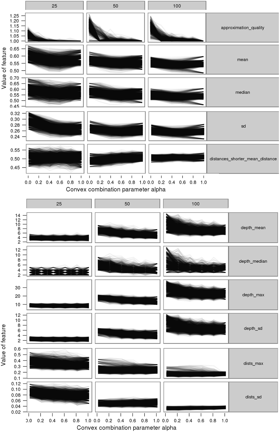
Figure 4. Feature variation with instance difficulty for some exemplary features from distance (top) and minimum spanning tree (bottom) feature groups for the default parameter setting (α = 1, β = 2).

Generally, for all three considered parameter settings, most features show similar patterns along the instance difficulty level. However, there are a few “contrast patterns” (i.e., the feature is increasing in value over instance difficulty for one parameter setting and decreasing for another parameter setting) observed among different parameter settings. For example, the distance mean and the SD show contrast patterns for the second parameter setting (α = 0, β = 4) from the other two (see Figure 5). Moreover, we observe that the sharp increasing pattern over the instance difficulty for the third parameter setting (α = 4, β = 0) has slowed down for the default parameter setting (α = 1, β = 2), and even converted to a decreasing pattern for the second setting. This provides strong evidence on the impact of parameters. Similar contrast patterns are observed in the other feature groups as well, such as the convex hull and nearest neighbor. These contrast patterns suggest the dependence of problem hardness on the algorithm parameters. This dependence further indicates that algorithms with different settings can have complementary problem-solving capabilities. We believe that such capabilities can provide insights into automatic parameter configuration. Therefore, we further investigate these capabilities by comparing the approximation ratios of the three algorithms achieved on each others’ easy and hard instances.

FIGURE 5

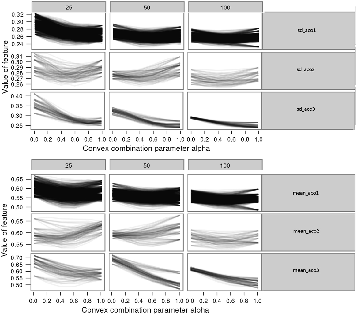
Figure 5. Feature variation with instance difficulty for mean (top) and SD (bottom) of distances for the three parameter settings 1 (top), 2 (middle), and 3 (bottom).

3.4. Comparison of the Parameter Settings

As shown in Figure 6, both the second (α = 0, β = 4) and the third (α = 4, β = 0) parameter settings have obtained worse approximation ratios for the easy instances of the first parameter setting (α = 1, β = 2) than the first parameter setting. In the case of the hard instances, the second parameter setting has achieved better approximation ratios than the first parameter setting itself. The outcomes of the other two cross-checks are comparable: given the hard instances of one algorithm configuration, the other two settings achieve better results. This is a strong support for our previous conjecture on the complementary capabilities of different parameter settings.

FIGURE 6

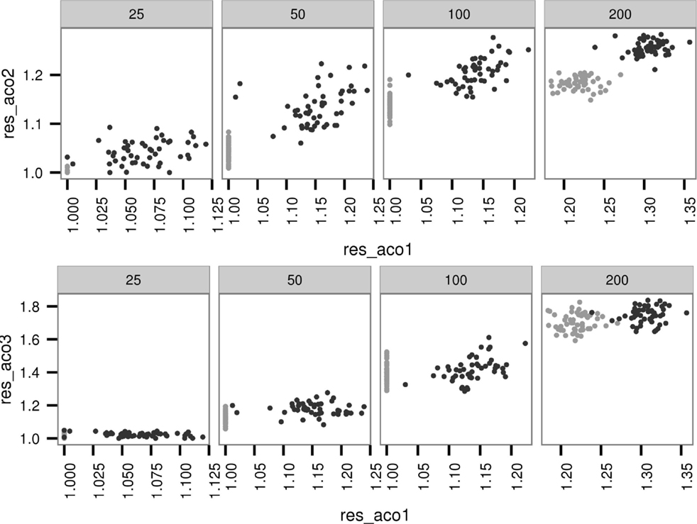
Figure 6. Performance of the second (res_aco2) parameter setting (top) and the third (res_aco3) parameter setting (bottom) on the easy (gray) and hard (black) instances of the first (res_aco1) parameter setting.

The outcomes of running the ACO algorithm with the first and the third parameter settings on the easy and hard instances of the second parameter setting follow a similar pattern to the previous experiment (see Figure 7). The results of the last comparative experiment on the instances of the third parameter setting are not significant that it merely follows the pattern for the first setting with worse approximation values. In summary, our comparisons suggest that the first and the second parameter settings complement each other, performing better on each other’s hard instances.

FIGURE 7

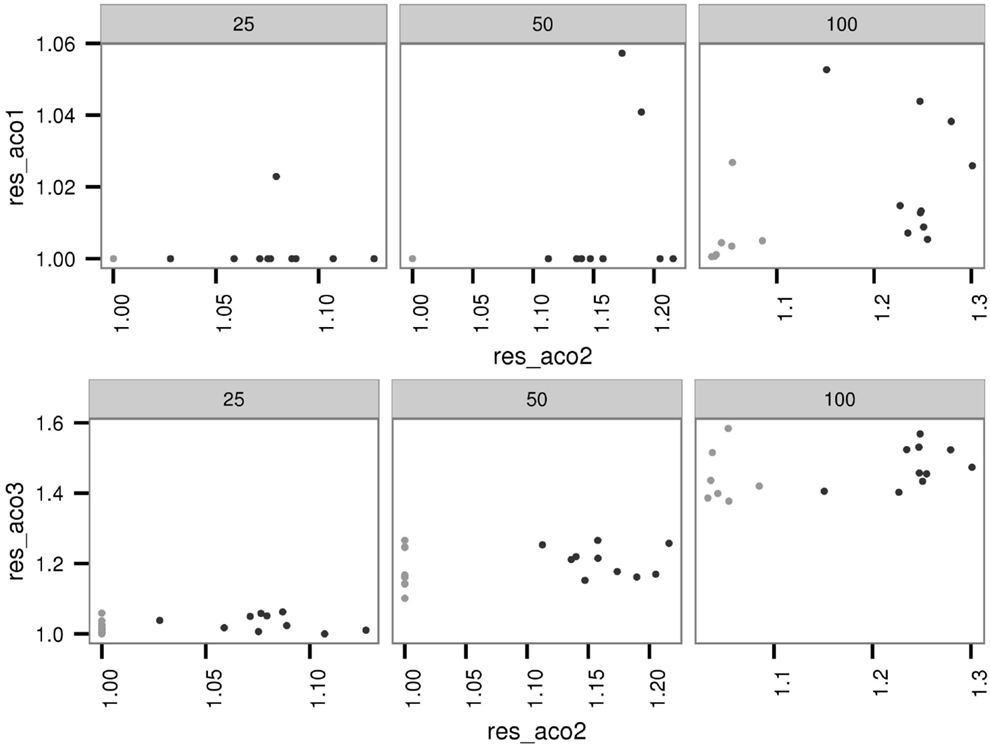
Figure 7. Performance of the first (res_aco1) parameter setting (top) and the third (res_aco3) parameter setting (bottom) on the easy (gray) and hard (black) instances of the second(res_aco2) parameter setting.

4. Extending the Analysis for ρ and n

For the analysis of ρ and n, we adhere to the experimental setup described in the above section. Similarly, we consider several parameter settings for our analysis based on varying ρ and n among feasible values. For one batch of instances, we keep the ρ fixed to 0.5 and evolved instances for three n values 5, 25, and 100, whereas in the other batch n is kept fixed to 25 and ρ is varied among 0.2, 0.5, and 0.8. The general idea behind the choice is that we have to isolate the conditions to investigate the effect, which is usually considered in traditional scientific experiments. Similar to the previous experiments, the remaining parameters are set to their default values (α = 1, β = 2) as in the original MMAS implementation by Stützle (2012). The instance generation is repeated, for instance, sizes 25 and 100.

As shown in the Figure 8, the mean angles between the adjacent cities for the easy instances are a bit higher than for hard instances. This difference widens with increasing number of ants as depicted in the middle row of the boxplots. In contrast to this, the difference narrows with increasing ρ for the fixed n = 25.

FIGURE 8

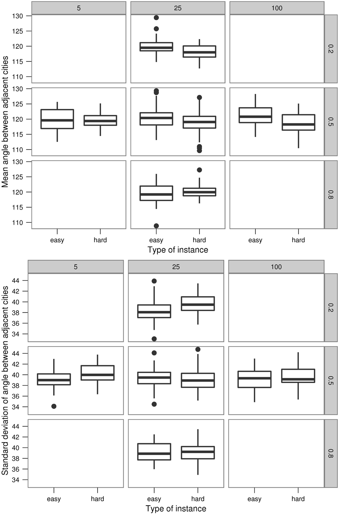
Figure 8. Boxplots of the means and the SDs of the angles between neighbor cities.

Figure 9 shows the means and SDs of the distances. For the fixed n = 25, the mean values of the easy instances are almost the same for different values of ρ, while the values of the hard instances vary. For the smallest ρ value (of 0.2), the hard instances have a higher mean value than easy instances and this difference decreases with the increasing ρ until 0.5 and the pattern inverts. Thus, for the largest ρ value (of 0.8), the mean of hard instances again has a higher value than of the easy instances. This pattern is reflected in the SDs as well. There, the hard instances initially have lower values than the easy instances. On the other hand, there is no significant variation shown over the increasing number of ants n for either the means or the SDs of distances.

FIGURE 9

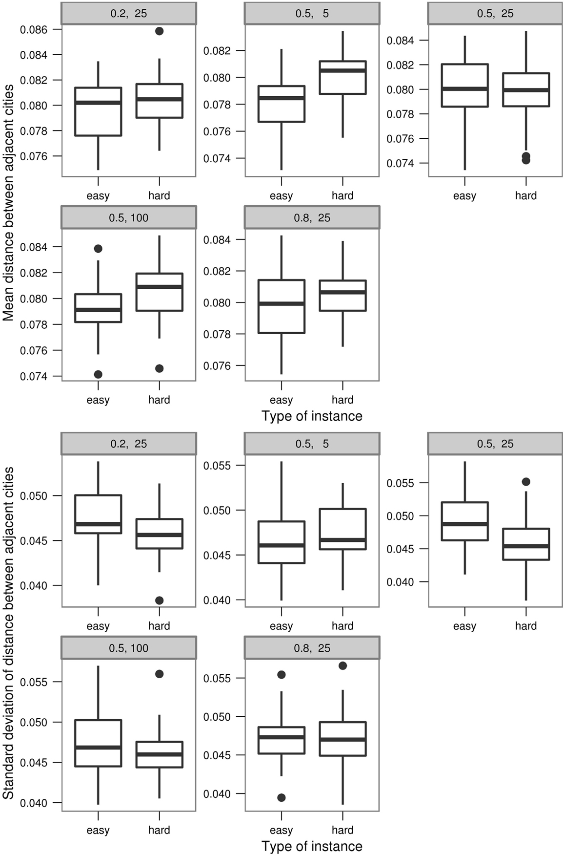
Figure 9. Boxplots of the means (top) and the SDs (bottom) of the distances.

Compared to the significant difference in the feature values of the easy and hard instances of parameter settings for varying α and β this difference is less. This indicates that n and ρ have less effect on the overall approximation ratio achieved by ACO compared to the effect from α and β. Nevertheless, the effect exists and is sufficiently strong to be observed in the current experiments. Therefore, we further study the capability of the feature data with varying ρ and n for parameter prediction.

5. Parameter Prediction

In order to build a reliable model, we significantly extend our collection of data gained from the experiments in Section 3. Around 3000 instances (10 instances per each category in hard/easy instances of size 100, and 144 parameter combinations for α, β ∈ {1,2,3,4}, ρ ∈ 0.2,0.5,0.8, n ∈ 5,25,100) are generated in order to build our prediction model.

5.1. The First Prediction Model

We build a simple prediction model merely as a proof of concept that a problem hardness model can be used for ACO parameter prediction. To achieve this, we use a popular basic technique for model building. A high-level overview of the model is shown in Figure 10. Instead of predicting the allegedly optimal parameters, we actually predict the approximation values given the 144 possible parameter combinations. Then, we select among those combinations the one that achieves the best approximation as the model’s output. Hence, the actual model construction is based on the approximation ratio as the dependent variable. Note that a similar model architecture is used in the recent work of Muñoz et al. (2012) for the prediction of algorithm performance based on landscape features and parameters. Note that any kind of instance set can be used to build a prediction model. However, a randomly generated or a benchmark instance set would not cover the full spectrum of difficulty. By evolving two sets of instances having extreme difficulty levels (hard and easy) and then generating instances with medium difficulty levels in between by morphing these hard and easy instances, we generate a diverse set of instances that covers the full spectrum of difficulty. This improves the overall prediction quality.

FIGURE 10

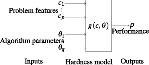
Figure 10. Prediction model 1. It predicts the algorithm performance based on the problem features c_i, 1 ≤ i ≤ p and the possible algorithm parameters θ_j, 1 ≤ j ≤ q.

To build our prediction model, we use the classical pattern classification technique introduced by Aha et al. (1991), which is implemented in the Weka data mining framework (Hall et al., 2009). In the training phase, we feed the generated instances into this nearest neighbor search-based classifier. As we have seen in the previous hardness analysis, not all problem features appear to be significantly different for easy and hard instances. We use the correlation-based feature subset selection method (Hall, 200) to select the most important features. These identified features for the training set are used to build the prediction model together with the parameter values and the respective approximation ratio. These are, namely, mean distance to centroid, number of inner points in the convex hull, distance mean, distance SD, minimum spanning tree distance SD, nearest neighbor distances mean, and the nearest neighbor distances median.

After the training phase, the model can reliably predict the performance for the parameter settings. We choose the parameter setting with the best predicted performance as the system output. The performance data for all parameter combinations for each TSP instance are considered for a statistical test later.

Table 2 shows some predicted approximation ratios of the model and the actual best approximation ratios. For all instances, the prediction error is <9% and for more than a half of the instances this error is even <1%.

TABLE 2

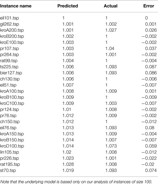
Table 2. Predicted and actual approximation ratios for 26 TSPLIB instances of size in range 51–264.

The performance predictions can be used to produce the final output of the prediction system that gives the best parameter combination, as described in the previous section. Accordingly, these respective outputs for the considered test set are shown in Table 3. For the majority of the instances, the best parameter setting is predicted. In other cases, there exist differences in at most two parameters, and the predicted setting in these cases is, in fact, the second best parameter setting.

TABLE 3

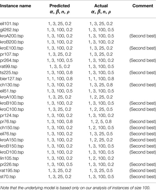
Table 3. Predicted and actual parameter settings (α, β, n, and ρ) for 26 TSPLIB instances of size in range 51–264.

Although our model cannot produce the best parameter setting for all instances, the raw approximation values for predicted and actual performance are very similar. Therefore, we conduct a rank test to check for any significant difference between the predicted values. We choose the Wilcoxon signed rank test (Wilcoxon, 1945), as there is no guarantee about the distribution, and the results are paired as they are based on the TSP instance on which the approximation ratio is obtained. For each TSP instance, the predicted and actual approximation ratios obtained for all parameter settings are considered for the test. For the test, we set the hypothesis that the predicted values are greater than the actual values. For all instances, the resulting p-values are reasonably large, and hence, the alternative hypothesis is rejected (see Table 4). Thus, we fail to reject the null hypothesis, meaning that both distributions are equal.

TABLE 4

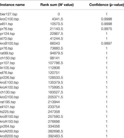
Table 4. Results of the Wilcoxon signed rank tests on the predicted and actual approximation ratios for all parameter combinations of the TSPLib instances, for the hypothesis “predicted > actual”, positive rank sum (W) and confidence (p) values are displayed accordingly.

5.2. More Effective Prediction Models

The initial prediction model discussed above has an implicit limitation. The internal model actually predicts the performance not the parameters, and hence, it is required to retrieve performance results for all parameter combinations. This means several calls are made to the prediction model for a given new instance. If the parameters can be independently determined, they can be predicted directly without predicting the performance first. In the following, we predict the parameters directly and analyze the results to study the effectiveness of this method.

The key idea of direct parameter prediction is to consider only the feature values and parameter settings with respect to the optimal performance. If this is possible, then we can directly map the feature values or the structure of these problem instances to the considered parameter values as shown in Figure 11. To obtain such a data set with optimal performance, we considered a subset of the instances for which the approximation ratio is exclusively between 1 and 1.001. The main idea behind this choice is to extract the input data representing only the optimal parameter values with respect to a given set of structural features. Such optimal parameter values are, in fact, the values that resulted in the optimal approximation ratio for the respective TSP instances. Hence, the parameter values with respect to the instances with optimal approximation values represent our input data set. Then, a model can be learned to predict optimal parameter values through supervised learning based on the received optimal parameter values for the feature values of the problem instances.

FIGURE 11

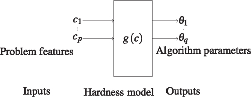
Figure 11. Prediction model 2. It predicts the algorithm parameters θ_j, 1 ≤ j ≤ q based on the problem features c_i, 1 ≤ i ≤ p on optimal performance.

Our goal of building a prediction model is to identify the capability of TSP instance features for parameter prediction of ACO. Hence, for simplicity, we again consider a model similar to our previous prediction model (see Figure 10) in which a single output is produced. By combining four such trained models to predict each parameter, we consider an integrated parameter prediction model. Hence, to obtain a prediction for a new instance, we invoke the model four times, a single call for each separate model. We call this prediction model 2a.

Our results for prediction model 2a indicate that optimal values for parameters cannot be predicted independently of other parameters. This is observed in incorrect predictions for the majority of the test instances (see Table 5). Compared to the other three parameters, the high-prediction precision for parameter α indicates that it is quite independent from the other parameters. To verify the nature of ACO parameters, we try in the following to predict each one of the parameters given the other parameters. For this, we again build four prediction models, where each model is trained with feature data and the values of all four parameters as inputs and having each considered parameter as the target. Similar to the former model, for this model also the features and the parameter data extracted only from the subset of the instances that the ACO algorithm obtained near optimal approximation ratio (almost 1). The predictions made by this model (we call this the prediction model 2b) are listed in Table 6.

TABLE 5

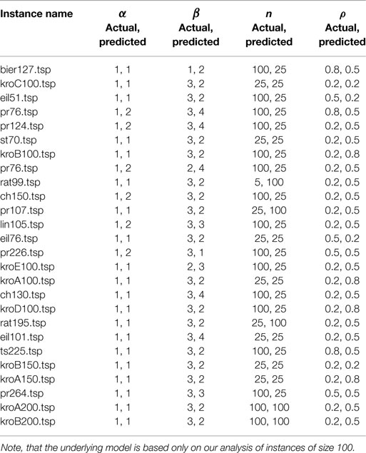
Table 5. Predicted and actual best parameter settings (α, β, n, and ρ) for 26 TSPLIB instances of size in range 51–264 from the prediction model 2a.

TABLE 6

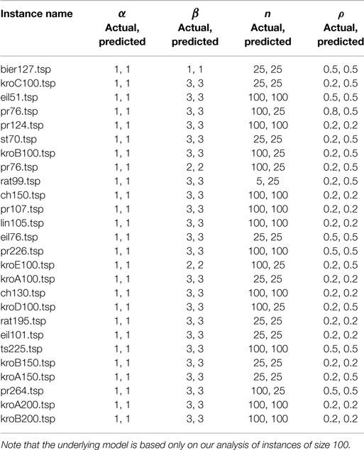
Table 6. Predicted and actual parameter settings (α, β, n, and ρ) for 26 TSPLIB instances of size in range 51–264 from the prediction model 2b.

For α and β, the exact correct result is predicted for all the instances, whereas the exact correct values are predicted for the majority of the cases for the other two parameters (see Table 6). The major difference when making a prediction with this model and the previous model is that this model additionally requires the optimal values of all the other parameters as the inputs while the previous model requires only the feature data as the inputs. The results show that the optimal value for a parameter can be predicted successfully given the optimal values for the other parameters, supporting our hypothesis that the ACO parameters are, in fact, interdependent on each other.

The prediction model 2b is built only as a proof of concept: it is not practical, since it requires the values of all other parameters as inputs to predict the optimal value for a given parameter. A practical model similar to our model 2a should take the dependencies among parameters into account internally and predict all parameters simultaneously. Building such a model is an interesting research direction although it is out of the scope of this study, hence, left as an open problem for future research. Furthermore, a theoretical analysis of this interdependency among the ACO parameters is essential, as it would provide a basis for such a novel prediction model.

As discussed in Section 2, this idea of using instance features for parameter prediction is rather novel in the ACO context. There are parameter tuning methods widely used in ACO context; however, our approach should be distinguished from tuning. It is observed that tuning often requires a substantial amount time to run the algorithm iteratively on a specified instance. In contrast, our approach requires time to calculate the feature values for the given TSP instance and to produce the prediction output for these features set, which is a single pass of the prediction model. Therefore, this approach is effective compared to a tuning based approach.

6. Conclusion

In this article, we have studied the problem hardness features of the TSP and some ACO algorithm parameters, their relationship and the impact on performance. First, we considered the parameters α and β that determine the importance of pheromone concentration and heuristic information, respectively. We have further extended the study to another two important ACO parameters: n the number of ants and ρ the pheromone update strength. From the feature-based analysis, it is observed that the effects of the latter two parameters are less significant compared to that of the former two. Furthermore, among the studied 47 instance features, a smaller subset is identified to be strongly correlated with the problem hardness for the TSP and ACO. Based on these features, we have built a prediction model to determine the values of the considered ACO parameters. Our investigations on a wide range of instances from TSPLIB show that the instance features allow for a reliable prediction of well-performing algorithm setups.

Additionally, as a result on the experimentation of the parameter prediction, this study provides some clue that there exist interdependencies among the ACO parameters. This motivates future work on theoretical analysis to study these dependencies among ACO parameters. Such a study would be able to provide deeper insights into ACO algorithm configuration for achieving an optimal performance.

Conflict of Interest Statement

The authors declare that the research was conducted in the absence of any commercial or financial relationships that could be construed as a potential conflict of interest.

Acknowledgments

We thank Bernd Bischl for early discussions, Heike Trautmann and Olaf Mersmann for their feedback on the preliminary version of this research. This research has been supported by the Australian Research Council (ARC) under grant agreement DP140103400.

References

Agarwala, R., Applegate, D., Maglott, D., Schuler, G., and Schffer, A. (2000). A fast and scalable radiation hybrid map construction and integration strategy. Genome Res. 10, 350–364. doi: 10.1101/gr.10.3.350

PubMed Abstract | CrossRef Full Text | Google Scholar

Aha, D. W., Kibler, D., and Albert, M. K. (1991). Instance-based learning algorithms. Mach. Learn. 6, 37–66. doi:10.1007/BF00153759

CrossRef Full Text | Google Scholar

Applegate, D., Cook, W. J., Dash, S., and Rohe, A. (2002). Solution of a min-max vehicle routing problem. J. Comput. 14, 132–143. doi:10.1287/ijoc.14.2.132.118

CrossRef Full Text | Google Scholar

Applegate, D. L., Bixby, R. E., Chvatal, V., and Cook, W. J. (2007). The Traveling Salesman Problem: A Computational Study (Princeton Series in Applied Mathematics). Princeton, NJ: Princeton University Press.

Google Scholar

Bailey, C. A., McLain, T. W., and Beard, R. W. (2000). “Fuel saving strategies for separated spacecraft interferometry,” in In AIAA Guidance, Navigation, and Control Conference. Denver, CO.

Google Scholar

Bland, R. G., and Shallcross, D. F. (1989). Large traveling salesman problem arising from experiments in x-ray crystallography: a preliminary report on computation. Oper. Res. Lett. 8, 125–128. doi:10.1016/0167-6377(89)90037-0

CrossRef Full Text | Google Scholar

Dorigo, M., and Stützle, T. (2004). Ant Colony Optimization. Scituate, MA: Bradford Company.

Google Scholar

Fischer, T., Stützle, T., Hoos, H., and Merz, P. (2005). “An analysis of the hardness of TSP instances for two high-performance algorithms,” in 6th Metaheuristics International Conference (MIC). Vienna, 361–367.

Google Scholar

Grtschel, M., Jnger, M., and Reinelt, G. (1991). Optimal control of plotting and drilling machines: a case study. Z. Oper. Res. 35, 61–84.

Google Scholar

Hall, M., Frank, E., Holmes, G., Pfahringer, B., Reutemann, P., and Witten, I. H. (2009). The weka data mining software: an update. SIGKDD Explor. Newsl. 11, 10–18. doi:10.1145/1656274.1656278

CrossRef Full Text | Google Scholar

Hall, M. A. (2000). “Correlation-based feature selection for discrete and numeric class machine learning,” in Proceedings of the Seventeenth International Conference on Machine Learning (San Francisco, CA: Morgan Kaufmann Publishers Inc.), 359–366.

Google Scholar

Hutter, F., Hoos, H. H., and Leyton-Brown, K. (2013). “Identifying key algorithm parameters and instance features using forward selection,” in Proceedings of the 7th International Conference on Learning and Intelligent Optimization (LION). Berlin Heidelberg.

Google Scholar

Karp, R. M. (2010). “Reducibility among combinatorial problems,” in 50 Years of Integer Programming 1958–2008 eds M. Jünger, T. M. Liebling, D. Naddef, G. L. Nemhauser, W. R. Pulleyblank, G. Reinelt (Berlin Heidelberg: Springer), 219–241. doi:10.1007/978-3-540-68279-0_8

CrossRef Full Text | Google Scholar

Kötzing, T., Neumann, F., Röglin, H., and Witt, C. (2012). Theoretical analysis of two ACO approaches for the traveling salesman problem. Swarm Intell. 6, 1–21. doi:10.1007/s11721-011-0059-7

CrossRef Full Text | Google Scholar

Kötzing, T., Neumann, F., Sudholt, D., and Wagner, M. (2011). “Simple max-min ant systems and the optimization of linear pseudo-Boolean functions,” in Proceedings of the 11th Workshop Proceedings on Foundations of Genetic Algorithms, FOGA (New York, NY: ACM), 209–218.

Google Scholar

Lenstra, J. K., and Rinnooy Kan, A. H. G. (1975). Some simple applications of the travelling salesman problem. Oper. Res. Q. 26, 717–733. doi:10.1057/jors.1975.151

PubMed Abstract | CrossRef Full Text | Google Scholar

Lin, S., and Kernighan, B. (1973). An effective heuristic algorithm for the traveling salesman problem. Oper. Res. 21, 498–516. doi:10.1287/opre.21.2.498

CrossRef Full Text | Google Scholar

López-Ibáñez, M., Dubois-Lacoste, J., Stützle, T., and Birattari, M. (2011). The Rpackage Irace Package, Iterated Race for Automatic Algorithm Configuration. Technical Report TR/IRIDIA/2011-004, IRIDIA. Belgium: Universite Libre de Bruxelles.

Google Scholar

López-Ibáñez, M., and Stützle, T. (2012). The automatic design of multi-objective ant colony optimization algorithms. IEEE Trans. Evol. Comput. 16, 861–875. doi:10.1093/bioinformatics/btu702

PubMed Abstract | CrossRef Full Text | Google Scholar

Mersmann, O., Bischl, B., Trautmann, H., Wagner, M., Bossek, J., and Neumann, F. (2013). A novel feature-based approach to characterize algorithm performance for the traveling salesperson problem. Ann. Math. Artif. Intell. 69, 151–182. doi:10.1007/s10472-013-9341-2

CrossRef Full Text | Google Scholar

Muñoz, M. A., Kirley, M., and Halgamuge, S. K. (2012). “A meta-learning prediction model of algorithm performance for continuous optimization problems,” in 12th International Conference on Parallel Problem Solving from Nature (PPSN) (Berlin Heidelberg: Springer-Verlag), 226–235.

Google Scholar

Nallaperuma, S., Wagner, M., and Neumann, F. (2014). “Parameter prediction based on features of evolved instances for ant colony optimization and the traveling salesperson problem,” in Parallel Problem Solving from Nature PPSN XIII, Volume 8672 of Lecture Notes in Computer Science, eds T. Bartz-Beielstein, J. Branke, B. Filipi and J. Smith (Berlin Heidelberg: Springer International Publishing), 100–109.

Google Scholar

Nallaperuma, S., Wagner, M., Neumann, F., Bischl, B., Mersmann, O., and Trautmann, H. (2013a). “A feature-based comparison of local search and the Christofides algorithm for the travelling salesperson problem,” in Proceedings of the Twelfth Workshop on Foundations of Genetic Algorithms XII, FOGA XII (New York, NY: ACM), 147–160.

Google Scholar

Nallaperuma, S., Wagner, M., and Neumann, F. (2013b). “Ant colony optimisation and the traveling salesperson problem: hardness, features and parameter settings (extended abstract),” in 15th Annual Conference Companion on Genetic and Evolutionary Computation Conference Companion (GECCO Companion) (New York, NY: ACM), 13–14.

Google Scholar

Pellegrini, P., Favaretto, D., and Moretti, E. (2006). “On max-min ant system’s parameters,” in 5th International Conference on Ant Colony Optimization and Swarm Intelligence (ANTS) (Berlin Heidelberg: Springer), 203–214.

Google Scholar

Pellegrini, P., Stützle, T., and Birattari, M. (2010). “Off-line vs. on-line tuning: a study on MAX – MIN ant System for the TSP,” in Swarm Intelligence (Berlin Heidelberg: Springer), 239–250.

Google Scholar

Pilat, M. L., and White, T. (2002). “Using genetic algorithms to optimize ACS-TSP,” in In Proceedings of the 3rd International Workshop on Ant Algorithms (ANTS) (London: Springer), 12–14.

Google Scholar

Plante, R. D., Lowe, T. J., and Chandrasekaran, R. (1987). The product matrix traveling salesman problem: an application and solution heuristic. Oper. Res. 35, 772–783. doi:10.1287/opre.35.5.772

CrossRef Full Text | Google Scholar

Ratliff, H. D., and Rosenthal, A. S. (1983). Order-picking in a rectangular warehouse: a solvable case of the traveling salesman problem. Oper. Res. 31, 507–521. doi:10.1287/opre.31.3.507

CrossRef Full Text | Google Scholar

Reinelt, G. (1991). TSPLIBA traveling salesman problem library. ORSA J. Comput. 3, 376–384. doi:10.1287/ijoc.3.4.376

CrossRef Full Text | Google Scholar

Ridge, E., and Kudenko, D. (2008). “Determining whether a problem characteristic affects heuristic performance,” in Recent Advances in Evolutionary Computation for Combinatorial Optimization, Vol. 153, Chap. 2. eds C. Cotta and J. van Hemert (Berlin: Springer), 21–35. doi:10.1007/978-3-540-70807-0

CrossRef Full Text | Google Scholar

Smith-Miles, K., and Lopes, L. (2012). Measuring instance difficulty for combinatorial optimization problems. Comput. Oper. Res. 39, 875–889. doi:10.1016/j.cor.2011.07.006

CrossRef Full Text | Google Scholar

Smith-Miles, K., van Hemert, J., and Lim, X. Y. (2010). “Understanding TSP difficulty by learning from evolved instances,” in 4th International Conference on Learning and Intelligent Optimization (LION) (Berlin Heidelberg: Springer), 266–280.

Google Scholar

Stützle, T. (2012). Software Package: ACOTSP.V1.03.tgz. Available at: http://iridia.ulb.ac.be/~mdorigo/ACO/aco-code/public-software.html

Google Scholar

Stützle, T., and Dorigo, M. (2002). A short convergence proof for a class of ant colony optimization algorithms. IEEE Trans. Evol. Comput. 6, 358–365. doi:10.1109/TEVC.2002.802444

CrossRef Full Text | Google Scholar

Stützle, T., and Hoos, H. H. (2000). Max-min ant system. Future Gener. Comput. Syst. 16, 889–914. doi:10.1016/S0167-739X(00)00043-1

CrossRef Full Text | Google Scholar

Stützle, T., López-Ibáñez, M., Pellegrini, P., Maur, M., Montes de Oca, M., Birattari, M., et al. (2012). “Parameter adaptation in ant colony optimization,” in Autonomous Search (Springer), 191–215.

Google Scholar

Wilcoxon, F. (1945). Individual comparisons by ranking methods. Biometrics Bull. 1, 80–83. doi:10.2307/3001968

CrossRef Full Text | Google Scholar