Hierarchical Quantification of Synergy in Channels

1. Introduction

In complex systems like biological networks, for example neural networks, a basic principle is that their functioning is based on the correlation and interaction of their different parts. While correlation between two sources is well understood, and can be quantified by Shannon’s mutual information (see, for example, Kakihara (1999)), there is still no generally accepted theory for interactions of three nodes or more. If we label one of the nodes as “output,” the problem is equivalent to determine how much two (or more) input nodes interact to yield the output. This concept is known in common language as “synergy,” which means “working together,” or performing a task that would not be feasible by the single parts separately.

There are a number of important works which address the topic, but the problem is still considered open. The first generalization of mutual information was interaction information (introduced in McGill (1954)), defined for three nodes in terms of the joint and marginal entropies:

$\begin{array}{l}I\left(X:Y:Z\right)=-H\left(X,Y,Z\right)+H\left(X,Y\right)+H\left(X,Z\right)+H\left(Y,Z\right)+\hfill \\ -H\left(X\right)-H\left(Y\right)-H\left(Z\right).\hfill \end{array}$ (1)

Interaction information is defined symmetrically on the joint distribution, but most approaches interpret it by looking at a channel, rather than a joint distribution, (X,Y) → Z. For example, we can rewrite equation (1) equivalently in terms of mutual information (choosing Z as “output”):

$I\left(X:Y:Z\right)=I\left(X,Y:Z\right)-I\left(X:Z\right)-I\left(Y:Z\right),$ (2)

where we see that it can mean intuitively “how much the whole (X,Y) gives more (or less) information about Z than the sum of the parts separately.” Another expression, again equivalent, is

$I\left(X:Y:Z\right)=I\left(X:Y|Z\right)-I\left(X:Y\right),$ (3)

which we can interpret as “how much conditioning over Z changes the correlation between X and Y ” (see Schneidmann et al. (2003a)). Unlike mutual information, interaction information carries a sign:

• I > 0: synergy. Conditioning on one node increases the correlation between the remaining nodes. Or, the whole gives more information than the sum of the parts. Example: XOR function.

• I < 0: redundancy. Conditioning on one node decreases, or explains away the correlation between the remaining nodes. Or, the whole gives less information than the sum of the parts. Example: X = Y = Z.

• I = 0: 3-independence. Conditioning on one node has no effect on the correlation between the remaining nodes. Or, the whole gives the same amount of information as the parts separately. The nodes can nevertheless still be conditionally dependent. Example: independent nodes.¹

As argued in Schneidmann et al. (2003b), Williams and Beer (2010), and Griffith and Koch (2014), however, this is not the whole picture. There are systems which exhibit both synergetic and redundant behavior, and interaction information only quantifies the difference of synergy and redundancy, with a priori no way to tell the two apart. In a system with highly correlated inputs, for example, the synergy would remain unseen, as it would be canceled by the redundancy. Moreover, this picture breaks down for more than three nodes. Another problem pointed out in Schneidmann et al. (2003b) and Amari (2001) is that redundancy (as for example in X = Y = Z) can be described in terms of pairwise interactions, not triple, while synergy (as in the XOR function) is purely threewise. Therefore, I compares and mixes information quantities of different nature.

A detailed explanation of the problem for two inputs is presented in Williams and Beer (2010) and it yields a decomposition (“Partial Information Decomposition,” PID) as follows: there exist two non-negative quantities, Synergy and Redundancy, such that

$I\left(X,Y:Z\right)=I\left(X:Z\right)+I\left(Y:Z\right)+\mathit{Syn}-\mathit{Red},$ (4)

or equivalently:

$I\left(X:Y:Z\right)=\mathit{Syn}-\mathit{Red}.$ (5)

Moreover, they define unique information for the inputs X and Y as

$\mathit{UI}\left(X\right)=I\left(X:Z\right)-\mathit{Red},$ (6)

$\mathit{UI}\left(Y\right)=I\left(Y:Z\right)-\mathit{Red},$ (7)

so that the total mutual information is decomposed positively:

$I\left(X,Y:Z\right)=\mathit{UI}\left(X\right)+\mathit{UI}\left(Y\right)+\mathit{Red}+\mathit{Syn}.$ (8)

What these quantities intuitively mean is

• Redundancy – information available in both inputs;

• Unique information – information available only in one of the inputs;

• Synergy – information available only when both inputs are present, arising purely from their interaction.

In this formulation, if one finds a measure of synergy, one can automatically define compatible measures of redundancy and unique information (and vice versa), provided that the measure of synergy is always larger or equal to I(X:Y :Z), and that the resulting measure of redundancy is less or equal than I(X:Z) and I(Y :Z). Synergy, redundancy, and unique information are defined on a channel, and choosing a different channel with the same joint distribution (e.g., (Y, Z) → X) may yield a different decomposition.

In Griffith and Koch (2014), an overview of (previous) measures of synergy and their shortcomings in standard examples is presented. In the same paper is then presented a newer measure for synergy, defined equivalently in Bertschinger et al. (2014) as

$\mathit{CI}\left(X,Y;Z\right):=I\left(X,Y:Z\right)-{\displaystyle \underset{p^{\ast }\in \wedge }{\min }}{I}_{p^{\ast }}\left(X,Y:Z\right),$ (9)

where ∧ is the space of distributions with prescribed marginals:

$\wedge =\left\{q\in P\left(X,Y,Z\right)|q\left(X,Z\right)=p\left(X,Z\right),q\left(Y,Z\right)=p\left(Y,Z\right)\right\}.$ (10)

This measure satisfies interesting properties (proven in Griffith and Koch (2014) and Bertschinger et al. (2014)), which make it compatible with Williams and Beer’s PID, and with the intuition in most examples. However, it was proven in Rauh et al. (2015) that such an approach can not work in the desired way for more than three nodes (two inputs).

Our approach uses information geometry (Amari and Nagaoka, 2000), extending previous work on hierarchical decompositions (Amari, 2001) and complexity (Ay, 2015). (Compare the related approach on information decomposition pursued in Harder et al. (2013).) The main tools of the present paper are KL-projections and the Pythagorean relation that they satisfy. This allows (as in Amari (2001)) to form hierarchies of interactions of different orders in a geometrical way. In the present problem, we decompose mutual information between inputs and outputs of a channel k, for two inputs, as

$I\left(X,Y:Z\right)=d_1\left(k\right)+d_2\left(k\right),$ (11)

where d₂ quantifies synergy (as in Equation (8)), and d₁ integrates all the lower order terms (UI, Red), quantifying the so-called union information (see Griffith and Koch (2014)). One may want to use this measure of synergy to form a complete decomposition analogous to Equation (8), but this does not work, as in general it is not true that d₂ ≤ I(X:Y :Z). For this reason, we keep the decomposition more coarse, and we do not divide union information into unique and redundant.

For more inputs X₁, … , X_N, the decomposition generalizes to

$I\left(X_1,\dots ,X_N:Z\right)=d_1\left(k\right)+\dots +d_N\left(k\right)={\displaystyle \sum _{i=1}^N}{d}_i\left(k\right),$ (12)

where higher orders of synergy appear.

Until now, there seems to be no way of rewriting the decomposition of Griffith and Koch (2014) and Bertschinger et al. (2014) in a way consistent with information geometry, and more in general, Williams and Beer’s PID seems hard to write as a geometric decomposition. A comparison between d₂ and the measure CI of Griffith and Koch (2014) and Bertschinger et al. (2014) is presented in Section 5. There we show that d₂ ≤ CI, and we argue, with a numerical example, that CI overestimates synergy at least in one case.

For a small number of inputs (≲ 5), our quantities are easily computable with the standard algorithms of information geometry (like iterative scaling (Csiszár and Shields, 2004)). This allowed us to get precise quantities for all the examples considered.

1.1. Technical Definitions

We consider a set of N input nodes V = {1, … , N}, taking values in the sets X₁, … , X_N, and an output node, taking values in the set Y. We write the input globally as X: = X₁ × … × X_N. For example, in biology, Y can be the phenotype and X can be a collection of genes determining Y. We denote by F(Y) the set of real functions on Y and with P(X) the set of probability measures on X.

We can model the channel from X to Y as a Markov kernel (called also stochastic kernel, transition kernel, or stochastic map) k, that assigns to each x ∈ X a probability measure on Y (for a detailed treatment, see Kakihara (1999)). Here, we will consider only finite systems, so we can think of a channel simply as a transition matrix (or stochastic matrix) whose rows sum to one.

$k\left(x;y\right)\ge 0\forall x,y;{\displaystyle \sum _y}k\left(x;y\right)=1\forall x.$ (13)

The space of channels from X to Y will be denoted by K(X;Y). We will denote by X and Y also the corresponding random variables, whenever this does not lead to confusion.

Conditional probabilities define channels: if p(X,Y) ∈ P(X,Y) and the marginal p(X) is strictly positive, then p(Y |X) ∈ K(X;Y) is a well-defined channel. Vice versa, if k ∈ K(X;Y), given p ∈ P(X) we can form a well-defined joint probability:

$\mathit{pk}\left(x,y\right):=p\left(x\right)k\left(x;y\right)\forall x,y.$ (14)

An “input distribution” p ∈ P(X) is crucial also to extend the notion of divergence from probability distributions to channels. The most natural way of doing it is the following.

Definition 1: Let p ∈ P(X), let k, m ∈ K(X;Y). Then

$D_p\left(k\left|\right|m\right):={\displaystyle \sum _{x,y}}p\left(x\right)k\left(x;y\right)\log \frac{k\left(x;y\right)}{m\left(x;y\right)}.$ (15)

Defined this way, D_p is affine in p. Moreover, it has an important compatibility property. Let p,q be joint probability distributions on X × Y, and let D be the KL-divergence. Then

$D\left(p\left(X,Y\right)\left|\right|q\left(X,Y\right)\right)=D\left(p\left(X\right)\left|\right|q\left(X\right)\right)+D_{p\left(X\right)}\left(p\left(Y|X\right)\left|\right|q\left(Y|X\right)\right).$ (16)

We will now illustrate our geometric ideas in channels with one, two, and three input nodes, and then we present some examples. The general case will be addressed in Section 4.

2. Geometric Idea of Synergy

2.1. Mutual Information as Motivation

It is a well-known fact in information theory that Shannon’s mutual information can be written as a KL-divergence:

$I_p\left(X:Y\right)=D\left(p\left(X,Y\right)\left|\right|p\left(X\right)p\left(Y\right)\right).$ (17)

From the point of view of information geometry, this can be interpreted as a “distance” between the real distribution and a product distribution that has exactly the same marginals, but maximal entropy (see Figure 1). In other words, we have

$I_p\left(X:Y\right)={\displaystyle \underset{\begin{array}{c}q\in P\left(X\right)\\ r\in P\left(Y\right)\end{array}}{\text{inf}}}D\left(p\left(X,Y\right)\left|\right|q\left(X\right)r\left(Y\right)\right).$ (18)

FIGURE 1

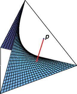
Figure 1. For two binary nodes, the family of product distributions is a surface in a 3-dimensional simplex.

The distribution given by p(X)p(Y) is optimal in the sense that

$p\left(X\right)p\left(Y\right)={\displaystyle \underset{\begin{array}{c}q\in P\left(X\right)\\ r\in P\left(Y\right)\end{array}}{\mathrm{arg\hspace{0.17em}}\min }}D\left(p\left(X,Y\right)\left|\right|q\left(X\right)r\left(Y\right)\right).$ (19)

The divergence between p and a submanifold is, as usual in geometry, the “distance” between p and the “closest point” on that submanifold, which in our case is the geodesic projection w.r.t. the mixture connection.

2.2. Extension to Channels

We can use the same insight with channels. Instead of a joint distribution on N nodes, we consider a channel from an input X to an output Y. Suppose we have a family $\mathcal{E}$ of channels, and a channel k that may not be in $\mathcal{E}$. Then, just as in geometry, we can define the “distance” between k and $\mathcal{E}$.

Definition 2: Let p be an input distribution. The divergence between a channel k and a family of channels $\mathcal{E}$ is given by

$D_p\left(k\left|\right|\mathcal{E}\right):={\displaystyle \underset{m\in \mathcal{E}}{\text{inf}}}{D}_p\left(k\left|\right|m\right).$ (20)

If the minimum is uniquely realized, we call the channel

${\mathrm{\pi }}_{\mathcal{E}}k:={\displaystyle \underset{m\in \mathcal{E}}{\mathrm{arg\hspace{0.17em}}\min }}{D}_p\left(k\left|\right|m\right)$ (21)

the KL-projection of k on $\mathcal{E}$ (and simply “a” KL-projection if it is not unique).

We will always work with compact families, so the minima will always be realized, and for strictly positive p they will be unique (see Section 4 for the details).

We will consider families $\mathcal{E}$ for which the KL-divergence satisfies a Pythagorean equality (see Figure 2 below for some intuition):

$D_p\left(k\left|\right|m\right)=D_p\left(k\left|\right|{\mathrm{\pi }}_{\mathcal{E}}k\right)+D_p\left({\mathrm{\pi }}_{\mathcal{E}}k\left|\right|m\right)$ (22)

for every m ∈ $\mathcal{E}$. These families (technically, closures of exponential families) are defined in Section 4.

FIGURE 2

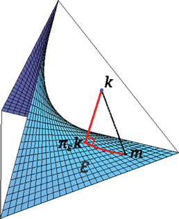
Figure 2. Illustration of the Pythagoras theorem for projections.

2.3. One Input

Consider first one-input node X, with input distribution p(X), and one output node Y. A constant channel k in K(X;Y) is a channel whose entries do not depend on X (more precisely: k(x;y) = k(x′;y) for any x,x′, y). This denomination is motivated by the following properties:

• They correspond to channels that do not use any information from the input to generate the output.

• The output distribution given by k is a probability distribution on Y which does not depend on X.

• Deterministic constant channels are precisely constant functions.

We call $\mathcal{E}$₀ the family of constant channels. Take now any channel k ∈ K(X;Y). If we want to quantify the dependence in k of Y on X, we can then look at the divergence of k from the constant channels:

$d_1\left(k\right):=D_p\left(k\left|\right|{\mathcal{E}}_0\right).$ (23)

The minimum is realized in ${\mathrm{\pi }}_{{\mathcal{E}}_0}k$. We have that

$d_1\left(k\right)=D_p\left(k\left|\right|{\mathrm{\pi }}_{{\mathcal{E}}_0}k\right)={\displaystyle \sum _{x,y}}p\left(x\right)k\left(x;y\right)\log \frac{k\left(x;y\right)}{{\mathrm{\pi }}_{{\mathcal{E}}_0}k\left(y\right)}$ (24)

$=H_{p{\mathrm{\pi }}_{{\mathcal{E}}_0}k}\left(Y\right)-H_{\mathit{pk}}\left(Y|X\right)=I_{\mathit{pk}}\left(X:Y\right),$ (25)

so that consistently with our intuition, the dependence of Y on X is just the mutual information. From the channel point of view, it is simply the divergence from the constant channels. (A rigorous calculation is done in Section 4.)

2.4. Two Inputs

Consider now two input nodes with input probability p and one output node. We can again define the family $\mathcal{E}$₀ of constant channels, and the same calculations give

$D_p\left(k\left|\right|{\mathcal{E}}_0\right)=I_{\mathit{pk}}\left(X_1,X_2:Y\right).$ (26)

This time, though, we can say a lot more: the quantity above can be decomposed. In analogy with the independence definition for probability distributions, we would like to define a split channel as a product channel of its parts: p(y|x₁, x₂) = p(y|x₁)p(y|x₂). Unfortunately, the term on the right would be in general not normalized, so we replace the condition by a weaker one. We call the channel k(X₁, X₂; Y) split if it can be written as

$k\left(x_1,x_2;y\right)={\mathrm{\varphi }}_0\left(x_1,x_2\right){\mathrm{\varphi }}_1\left(x_1;y\right){\mathrm{\varphi }}_2\left(x_2;y\right)$ (27)

for some functions ϕ₀, ϕ₁, and ϕ₂, which in general are not themselves channels (in particular, ϕ_i(x_i; y) ≠ p(y|x_i)). We call $\mathcal{E}$₁ the family of split channels. This family corresponds to those channels that do not have any synergy. This is a special case of an exponential family, analogous to the family of product distributions of Figure 1. The examples “single node” and “split channel” in the next section belong exactly to this family. Take now any channel k(X₁, X₂; Y). In analogy with mutual information, we call synergy the divergence:

$d_2\left(k\right):=D_p\left(k\left|\right|{\mathcal{E}}_1\right).$ (28)

Simply speaking, our synergy is quantified as the deviation of the channel from the set $\mathcal{E}$₁ of channels without synergy.

We can now project k first to $\mathcal{E}$₁, and then to $\mathcal{E}$₀. Since $\mathcal{E}$₀ is a subfamily of $\mathcal{E}$₁, the following Pythagoras relation holds from Equation (22):

$D_p\left(k\left|\right|{\mathrm{\pi }}_{{\mathcal{E}}_0}k\right)=D_p\left(k\left|\right|{\mathrm{\pi }}_{{\mathcal{E}}_1}k\right)+D_p\left({\mathrm{\pi }}_{{\mathcal{E}}_1}k\left|\right|{\mathrm{\pi }}_{{\mathcal{E}}_0}k\right).$ (29)

If, in analogy with the one-input case, we call the last quantity d₁, we get from Equations (26) and (28):

$I_{\mathit{pk}}\left(X_1,X_2:Y\right)=d_2\left(k\right)+d_1\left(k\right).$ (30)

The term d₁ measures how much information comes from single nodes (but it does not tell which nodes). The term d₂ measures how much information comes from the synergy of X₁ and X₂ in the channel. The example “XOR” in the next section will show this.

If we call $\mathcal{E}$₂ the whole K(X;Y), we get $\mathcal{E}$₀ ⊂ $\mathcal{E}$₁ ⊂ $\mathcal{E}$₂ and

$d_i\left(k\right):=D_p\left({\mathrm{\pi }}_{{\mathcal{E}}_i}k\left|\right|{\mathrm{\pi }}_{{\mathcal{E}}_{i-1}}k\right).$ (31)

2.5. Three Inputs

Consider now three nodes X₁, X₂, and X₃ with input probability p and a channel k. We have again

$D_p\left(k\left|\right|{\mathcal{E}}_0\right)=I_{\mathit{pk}}\left(X_1,X_2,X_3:Y\right).$ (32)

This time we can decompose the mutual information in different ways. We can, for example, look at split channels, i.e., in the form:

$k\left(x_1,x_2,x_3;y\right)={\mathrm{\varphi }}_0\left(x\right){\mathrm{\varphi }}_1\left(x_1;y\right){\mathrm{\varphi }}_2\left(x_2;y\right){\mathrm{\varphi }}_3\left(x_3;y\right)$ (33)

for some ϕ₀, ϕ₁, ϕ₂, and ϕ₃. As in the previous case, we call this family $\mathcal{E}$₁. Or we can look at more interesting channels, the ones in the form:

$k\left(x_1,x_2,x_3;y\right)={\mathrm{\varphi }}_0\left(x\right){\mathrm{\varphi }}_{12}\left(x_1,x_2;y\right){\mathrm{\varphi }}_{13}\left(x_1,x_3;y\right){\mathrm{\varphi }}_{23}\left(x_2,x_3;y\right)$ (34)

for some ϕ₀, ϕ₁₂, ϕ₁₃, and ϕ₂₃. We call this family $\mathcal{E}$₂, and it is easy to see that

${\mathcal{E}}_0\subset {\mathcal{E}}_1\subset {\mathcal{E}}_2\subset {\mathcal{E}}_3,$ (35)

where $\mathcal{E}$₀ denotes again the constant channels, and $\mathcal{E}$₃ denotes the whole K(X;Y). We define again

$d_i\left(k\right):=D_p\left({\mathrm{\pi }}_{{\mathcal{E}}_i}k\left|\right|{\mathrm{\pi }}_{{\mathcal{E}}_{i-1}}k\right).$ (36)

This time, the Pythagorean relation can be nested, and it gives us

$I_{\mathit{pk}}\left(X_1,X_2,X_3:Y\right)=d_3\left(k\right)+d_2\left(k\right)+d_1\left(k\right).$ (37)

The difference between pairwise synergy and threewise synergy is shown in the “XOR” example in the next section.

Now that we have introduced the measure for a small number of inputs, we can study the examples from the literature (Griffith and Koch, 2014) and show that our measure is consistent with the intuition. The general case will be more in rigor introduced in Section 4.

3. Examples

Here, we present some examples of decomposition for well-known channels. All the quantities have been computed using an algorithm analogous to iterative scaling (as in Csiszár and Shields (2004)).

3.1. Single Node Channel

The easiest example is considering a channel which only depends on X₁, i.e.,

$I\left(X:Y\right)=I\left(X_1:Y\right).$ (38)

For example, consider 3 binary input nodes X₁, X₂, and X₃ with constant input probability and one binary output node Y which is an exact copy of X₁.

Then, we have exactly one bit of single node information and no higher order terms (see Figure 3). Geometrically, k lies in $\mathcal{E}$₁, so the only non-zero divergence in equation (37) is d₁(k). As one would expect, d₂(k) and d₃(k) vanish, as there is no synergy of orders 2 and 3.

FIGURE 3

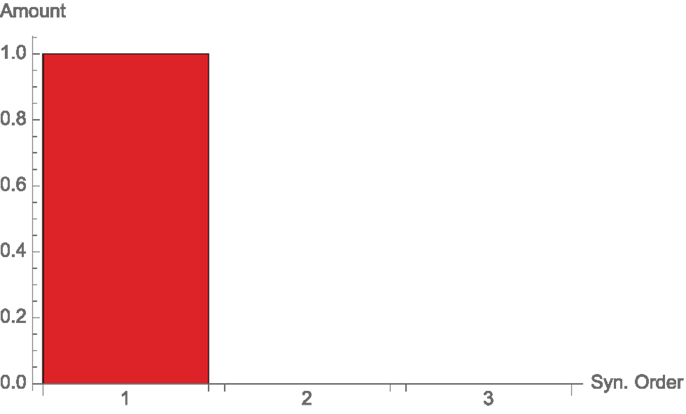
Figure 3. Synergies of different orders for the single-node channel, Example 3.1.

3.2. Split Channel

The second easiest example is a more general channel which obeys equation (33). In particular, consider 3 binary input nodes X₁, X₂, and X₃ with constant input probability (so, the x_i are independent), and output Y = X₁ × X₂ × X₃. As channel, we simply take the identity map (x₁, x₂, x₃) ↦ (x₁, x₂, x₃) ∈ Y. In this particular case:

$I\left(X:Y\right)={\displaystyle \sum _i}I\left(X_i;Y\right).$ (39)

We have 3 bits of mutual information (see Figure 4), which are all single node (but from different nodes). Since

$k\left(x_1,x_2,x_3;y\right)={\mathrm{\varphi }}_1\left(x_1;y_1\right){\mathrm{\varphi }}_2\left(x_2;y_2\right){\mathrm{\varphi }}_3\left(x_3;y_3\right),$ (40)

which is a special case of Equation (33), k ∈ $\mathcal{E}$₁, and so d₂(k) and d₃(k) in Equation (37) are again zero.

FIGURE 4

Figure 4. Synergies of different orders for the split channel, Example 3.2.

3.3. Correlated Inputs

Consider 3 perfectly correlated binary nodes, each one with uniform marginal probability. As output take a perfect copy of one (hence, all) of the inputs. We have again one bit of mutual information, which could come from any of the nodes, but no synergy, as no two nodes are interacting in the channel. The input distribution has correlation, but this has no effect on the channel, since the channel is simply copying the value of X₁ (or X₂ or X₃, equivalently). Therefore, again k ∈ $\mathcal{E}$₁. Of the terms in Equation (37), again the only non-zero is d₁(k) (see Figure 5).

FIGURE 5

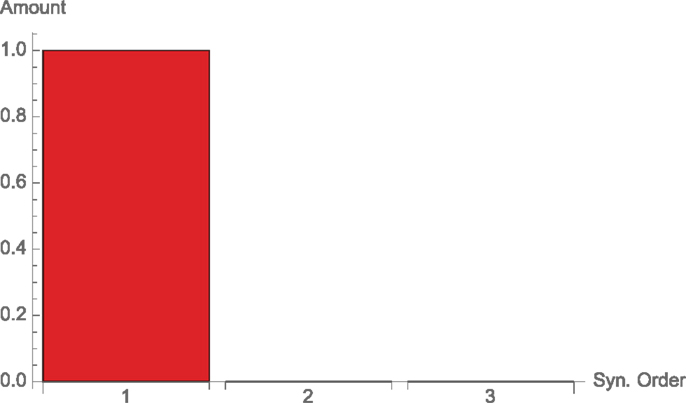
Figure 5. Synergies of different orders for correlated inputs, Example 3.3.

This example in the literature is used to motivate the notion of redundancy. A “redundant channel” is in our decomposition exactly equivalent to a single node channel, since it contains exactly the same amount of information.

3.4. Parity (XOR)

The standard example of synergy is given by the XOR function and more generally by the parity function between two or more nodes.

For example, consider 3 binary input nodes X₁, X₂, and X₃ with constant input probability, and one binary output node Y which is given by X₁ ⊻ X₂. We have 1 bit of mutual information, which is purely arising from a pairwise synergy (of X₁ and X₂), so this time k ∈ $\mathcal{E}$₂. The function XOR is pure synergy, so d₂(k) is the only non-zero term in Equation (37) (see Figure 6).

FIGURE 6

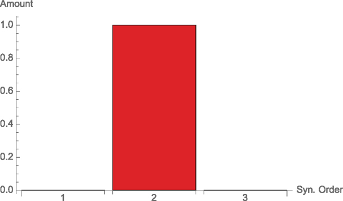
Figure 6. Synergies of different orders for the binary XOR function, Example 3.4.

If instead Y is given by the threewise parity function, or X₁ ⊻ X₂ ⊻ X₃, we have again 1 bit of mutual information, which now is purely arising from a threewise synergy, so here k ∈ $\mathcal{E}$₃, and the only non-zero term in Equation (37) is d₃(k) (see Figure 7).

FIGURE 7

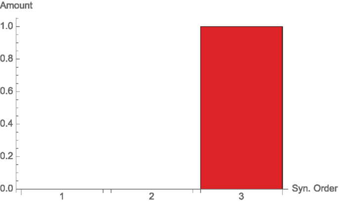
Figure 7. Synergies of different orders for the three wise parity function, Example 3.4.

In these examples, there are no terms of lower order synergy, but the generic elements of $\mathcal{E}$₂ and $\mathcal{E}$₃ usually do contain a non-zero lower part. Consider, for instance, the next example.

3.5. AND and OR

The other two standard logic gates, AND and OR, share the same decomposition. Consider two binary nodes X₁, and X₂ with uniform probability, and let Y be X₁ ∨ X₂ (or X₁ ∧ X₂). There is again one bit of mutual information, which comes mostly from single nodes, but also from synergy (see Figure 8).

FIGURE 8

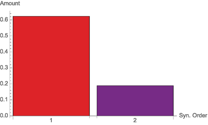
Figure 8. Synergies of different orders for the AND (and OR) function, Example 3.5.

Geometrically, this means that AND and OR are channels in $\mathcal{E}$₂, which lie close to the submanifold $\mathcal{E}$₁.

3.6. XorLoses

Here, we present a slightly more complicated example, coming from Griffith and Koch (2014). We have three binary nodes X₁, X₂, and X₃, where X₁ and X₂ have uniform probabilities, and an output node Y = X₁ ⊻ X₂, just like in the “XOR” example. Now we take X₃ to be perfectly correlated with Y = X₁ ⊻ X₂, so that Y could get the information either from X₃ or from the synergy between X₁ and X₂. We have one bit of mutual information, which can be seen as entirely coming from X₃, and so the synergy between X₁ and X₂ is not adding anything (see Figure 9).

FIGURE 9

Figure 9. Synergies of different orders for the XorLoses channel, Example 3.6.

3.7. XorDuplicate

Again from Griffith and Koch (2014), we have 3 binary nodes X₁, X₂, and X₃, where X₁ and X₂ have uniform probabilities, while X₃ = X₁. The output is X₁ ⊻ X₂ = X₃ ⊻ X₂, so it could get the information either from the synergy between X₁ and X₂ or X₂ and X₃. There is one bit of mutual information, which is coming from a pairwise interaction (see Figure 10). Again, it does not matter between whom.

FIGURE 10

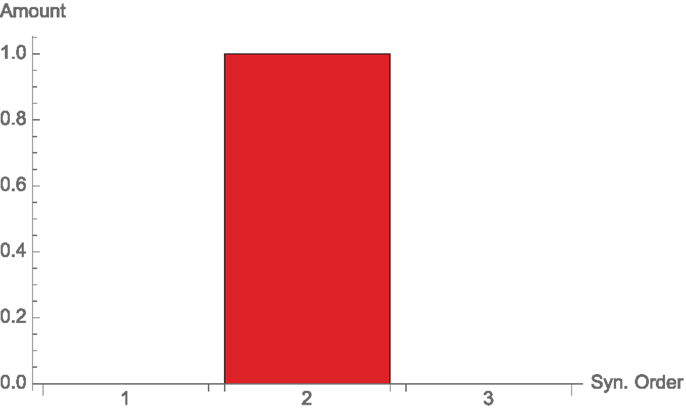
Figure 10. Synergies of different orders for the XorDuplicate channel, Example 3.7.

It should be clear from the examples here that decomposing only by order, and not by the specific subsets, is crucial. For example, in the “input correlation” example, there is no natural way to decide from which single node the information comes, even if it is clear that the interaction is of order 1.

4. General Case

Here, we try to give a general formulation, for N inputs, of the quantities defined in Section 2. As in the Section “Introduction,” we call the set of input nodes V of cardinality N, and we consider a subset I of the nodes. We denote the joint random variable (X_i, i ∈ I) by X_I, and we denote the complement of I in V by I^c. The case N = 3 in Section 2 should motivate the following definition.

Definition 3: Let I ⊆ V. We call F_I the space of functions that only depend on X_I and Y :

$F_I:=\left\{f\in F\left(X,Y\right)|f\left(x_I,x_{I^c};y\right)=f\left(x_I,{x\prime }_{I^c};y\right)\forall x_{I^c},{x\prime }_{I^c}\right\}.$ (41)

Let 0 ≤ i ≤ N. We call F_i the space of channels which can be written as a product of functions of F_I with the order of I at most i:

${\mathcal{E}}_i:=\mathit{cl}\left\{k\in K\left(X;Y\right)|\exists {\mathrm{\varphi }}_I\in F_I,{\mathrm{\varphi }}_0\in F\left(X\right)|k={\mathrm{\varphi }}_0{\displaystyle \prod _I}{\mathrm{\varphi }}_I;\left|I\right|\le i\right\},$ (42)

where cl denotes the closure in K(X;Y). Intuitively, this means that $\mathcal{E}$_i does not only contain terms in the form given in the curly brackets, but also limits of such terms. Stated differently, the closure of a set includes not only the set itself, but also its boundary. This is important because when we project to a family, the projection may lie on the boundary. In order for the result to exist, the boundary must then be included.

This way:

• $\mathcal{E}$₀ is the space of constant channels;

• $\mathcal{E}$ _N is the whole K(X;Y);

• $\mathcal{E}$_i ⊆ $\mathcal{E}$_j if and only if i ≤ j;

• For N ≤ 3 we recover exactly the quantities of Section 2.

The family $\mathcal{E}$_i is also the closure of the family in the form:

$\left\{\frac{1}{Z\left(X\right)}\exp \left({\displaystyle \sum _I}{f}_I\left(X;Y\right)\right)|f_I\in F_I;|I|\le i\right\},$ (43)

where

$Z\left(x\right):={\displaystyle \sum _y}\exp \left({\displaystyle \sum _I}{f}_I\left(x;y\right)\right).$ (44)

Such families are known in the literature as exponential families (see, for example, Amari and Nagaoka (2000)). In particular, it is compact (for finite N), so that the infimum of any function on $\mathcal{E}$_i is always a minimum. This means that for a channel k and an input distribution p:

$D_p\left(k\left|\right|{\mathcal{E}}_i\right):={\displaystyle \underset{m\in {\mathcal{E}}_i}{\text{inf}}}{D}_p\left(k\left|\right|m\right)={\displaystyle \underset{m\in {\mathcal{E}}_i}{\min }}{D}_p\left(k\left|\right|m\right)$ (45)

always exists. If it is unique, for example if p is strictly positive, we define the unique KL-projection as

${\mathrm{\pi }}_{{\mathcal{E}}_i}k:={\displaystyle \underset{m\in {\mathcal{E}}_i}{\mathrm{arg\hspace{0.17em}}\min }}{D}_p\left(k\left|\right|m\right).$ (46)

${\mathrm{\pi }}_{{\mathcal{E}}_i}k$ has the property that it defines the same output probability on Y.

Definition 4: Let k ∈ K(X;Y), let 1 ≤ i ≤ N. Then the i-wise synergy of k is (if the KL-projections are unique):

$d_i\left(k\right):=D_p\left({\mathrm{\pi }}_{{\mathcal{E}}_i}k\left|\right|{\mathrm{\pi }}_{{\mathcal{E}}_{i-1}}k\right).$ (47)

For more clarity, we call the 1-wise synergy “single node information” or “single-node dependence.”

For k ∈ K(X;Y) = $\mathcal{E}$_N, we can look at its divergence from $\mathcal{E}$₀. If we denote ${\mathrm{\pi }}_{{\mathcal{E}}_0}k$ by k₀:

$D_p\left(k\left|\right|{\mathcal{E}}_0\right)=D_p\left(k\left|\right|k_0\right)={\displaystyle \sum _{x,y}}p\left(x\right)k\left(x;y\right)\log \frac{k\left(x;y\right)}{k_0\left(y\right)}.$ (48)

If k is not strictly positive, we take the convention 0 log(0/0) = 0, and we discard the zero terms from the sum. Since the output distributions are the same, but k₀ is constant in x, it can not happen that for some (x;y), k₀(x;y) = 0 but k(x;y) ≠ 0. (The very same is true for all KL-projections ${\mathrm{\pi }}_{{\mathcal{E}}_i}k$, since $D_p\left({\mathrm{\pi }}_{{\mathcal{E}}_i}k\left|\right|k_0\right)\le D_p\left(k\left|\right|k_0\right)$.) For all other terms, Equation (48) becomes:

$D_p\left(k\left|\right|{\mathcal{E}}_0\right)={\displaystyle \sum _{x,y}}p\left(x\right)k\left(x;y\right)\log \mathrm{\hspace{0.17em}k}\left(x;y\right)-{\displaystyle \sum _{x,y}}p\left(x\right)k\left(x;y\right)\log k_0\left(y\right)$ (49)

$=-H_{\mathit{pk}}\left(Y|X\right)-{\displaystyle \sum _y}{k}_{\ast }p\left(y\right)\log k_0\left(y\right)$ (50)

$=-H_{\mathit{pk}}\left(Y|X\right)-{\displaystyle \sum _y}{k_0}_{\ast }p\left(y\right)\log k_0\left(y\right)$ (51)

$=-H_{\mathit{pk}}\left(Y|X\right)+H_{{k_0}_{\ast }p}\left(Y\right)=-H_{\mathit{pk}}\left(Y|X\right)+H_{k_{\ast }p}\left(Y\right)$ (52)

$=I_{\mathit{pk}}\left(X:Y\right).$ (53)

On the other hand, the Pythagorean relation (22) implies:

$D_p\left(k\left|\right|k_0\right)=D_p\left(k\left|\right|{\mathrm{\pi }}_{{\mathcal{E}}_{N-1}}k\right)+D_p\left({\mathrm{\pi }}_{{\mathcal{E}}_{N-1}}k\left|\right|k_0\right),$ (54)

and iterating:

$D_p\left(k\left|\right|k_0\right)=D_p\left(k\left|\right|{\mathrm{\pi }}_{{\mathcal{E}}_{N-1}}k\right)+D_p\left({\mathrm{\pi }}_{{\mathcal{E}}_{N-1}}k\left|\right|{\mathrm{\pi }}_{{\mathcal{E}}_{N-2}}k\right)+\dots +D_p\left({\mathrm{\pi }}_{{\mathcal{E}}_1}k\left|\right|k_0\right).$ (55)

In the end, we get

$I\left(X:Y\right)={\displaystyle \sum _{i=1}^N}{D}_p\left({\mathrm{\pi }}_{{\mathcal{E}}_i}k\left|\right|{\mathrm{\pi }}_{{\mathcal{E}}_{i-1}}k\right)={\displaystyle \sum _{i=1}^N}{d}_i\left(k\right).$ (56)

This decomposition is always non-negative, and it depends on the input distribution. The terms in Equation (56) can be in general difficult to compute exactly. Nevertheless, they can be approximated with iterative procedures.

5. Comparison with Two Recent Approaches

The measure of synergy, or respectively complementary information, defined in Griffith and Koch (2014) and Bertschinger et al. (2014) is

$C{I}_p\left(Y:X_1,X_2\right):=I_p\left(Y:X_1,X_2\right)-{\displaystyle \underset{p^{\ast }\in \wedge }{\min }}{I}_{p^{\ast }}\left(Y:X_1,X_2\right),$ (57)

where ∧ is the space of prescribed marginals:

$\wedge =\left\{q\in P\left(X_1,X_2,Y\right)|q\left(X_1,Y\right)=p\left(X_1,Y\right),q\left(X_2,Y\right)=p\left(Y_2,Y\right)\right\}.$ (58)

Our measure of synergy can be written, for two inputs, in a similar form:

$d_2\left(k\right)=D_p\left(k\left|\right|{\mathrm{\pi }}_{{\mathcal{E}}_1}k\right)=I_p\left(Y:X_1,X_2\right)-{\displaystyle \underset{p^{\ast }\in △}{\min }}{I}_{p^{\ast }}\left(Y:X_1,X_2\right),$ (59)

where △, in addition to the constraints of ∧, prescribes also the input:

$\begin{array}{l}△=\{q\in P\left(X_1,X_2,Y\right)|\hfill \\ q\left(X_1,Y\right)=p\left(X_1,Y\right),q\left(X_2,Y\right)=p\left(Y_2,Y\right),q\left(X_1,X_2\right)=p\left(X_1,X_2\right)\}.\hfill \end{array}$ (60)

Clearly △ ⊆ ∧, so

${\displaystyle \underset{p^{\ast }\in △}{\min }}{I}_{p^{\ast }}\left(Y:X_1,X_2\right)\ge {\displaystyle \underset{p^{\ast }\in \wedge }{\min }}{I}_{p^{\ast }}\left(Y:X_1,X_2\right),$ (61)

which implies that

$d_2\left(k\right)\le C{I}_p\left(Y:X_1,X_2\right).$ (62)

We argue that not prescribing the input leads to overestimating synergy, because the subtraction in Equation (57) includes a possible difference in the correlation of the input distributions.

For example, consider X₁, X₂, Y binary and correlated, but not perfectly correlated. (For perfectly correlated nodes, as in Section 3, △ = ∧, so there is no difference between the two measures.) In detail, consider the channel:

$k_{\mathrm{\beta }}\left(x_1,x_2;y\right):=\frac{\exp \left(\mathrm{\beta }y\left(x_1+x_2\right)\right)}{{\sum }_{y\prime }\exp \left(\mathrm{\beta }y\prime \left(x_1+x_2\right)\right)},$ (63)

and the input distribution:

$p_{\mathrm{\alpha }}\left(x_1,x_2\right):=\frac{\exp \left(\mathrm{\alpha }{x}_1{x}_2\right)}{{\sum }_{{x\prime }_1,{x\prime }_2}\exp \left(\mathrm{\alpha }{x\prime }_1{x\prime }_2\right)}.$ (64)

For α, β → ∞, the correlation becomes perfect, and the two measures of synergy are both zero. For 0 < α, β < ∞, our measure d₂(k_β) is zero, as clearly k_β ∈ $\mathcal{E}$₁. CI is more difficult to compute, but we can give a (non-zero) lower bound in the following way. First, we fix two values β = β₀, α = α₀. We consider the joint distribution $p_{{\mathrm{\alpha }}_0}{k}_{{\mathrm{\beta }}_0}$, and look at the marginals:

$p_{{\mathrm{\alpha }}_0}{k}_{{\mathrm{\beta }}_0}\left(X_1,Y\right),p_{{\mathrm{\alpha }}_0}{k}_{{\mathrm{\beta }}_0}\left(X_2,Y\right).$ (65)

We define the family ∧ as the set of joint probabilities which have exactly these marginals. If we increase β, we can always find an α such that the marginals do not change:

$p_{\mathrm{\alpha }}{k}_{\mathrm{\beta }}\left(X_1,Y\right)=p_{{\mathrm{\alpha }}_0}{k}_{{\mathrm{\beta }}_0}\left(X_1,Y\right),p_{\mathrm{\alpha }}{k}_{\mathrm{\beta }}\left(X_2,Y\right)=p_{{\mathrm{\alpha }}_0}{k}_{{\mathrm{\beta }}_0}\left(X_2,Y\right),$ (66)

i.e., such that p_α k_β ∈ ∧. Now we can look at the mutual information of p_α k_β and of $p_{{\mathrm{\alpha }}_0}{k}_{{\mathrm{\beta }}_0}$. If they differ, and (for example) the former is larger, then

$\begin{array}{l}{I}_{p_{\mathrm{\alpha }}{k}_{\mathrm{\beta }}}\left(Y:X_1,X_2\right)-I_{p_{{\mathrm{\alpha }}_0}{k}_{{\mathrm{\beta }}_0}}\left(Y:X_1,X_2\right)\hfill \\ \le I_{p_{\mathrm{\alpha }}{k}_{\mathrm{\beta }}}\left(Y:X_1,X_2\right)-{\displaystyle \underset{p^{\ast }\in \wedge }{\min }}{I}_{p^{\ast }}\left(Y:X_1,X_2\right)=C{I}_{p_{\mathrm{\alpha }}{k}_{\mathrm{\beta }}}\hfill \end{array}$ (67)

is a well-defined lower bound for $C{I}_{p_{\mathrm{\alpha }}{k}_{\mathrm{\beta }}}$. With a numerical simulation, we can show graphically that the mutual information is indeed not constant within the families ∧ (see Figure 11).

FIGURE 11

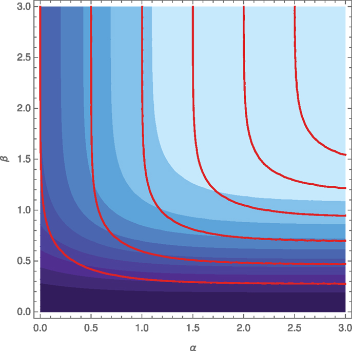
Figure 11. Mutual information and fixed marginals. The shades of blue represent the amount of I_p(Y :X₁,X₂) as a function of α,β (brighter is higher). Each red line represents a family ∧ of fixed marginals. While the lines of fixed mutual information and the families of fixed marginals look qualitatively similar, they do not coincide exactly, which means that I_p varies within the ∧.

From the picture, we can see that the red lines (families ∧ for different initial values) approximate well the lines of constant mutual information, at least qualitatively, but they are not exactly equal. This means that for most points p of ∧, the quantity:

$C{I}_p\left(Y:X_1,X_2\right):=I_p\left(Y:X_1,X_2\right)-{\displaystyle \underset{p^{\ast }\in \wedge }{\min }}{I}_{p^{\ast }}\left(Y:X_1,X_2\right)$ (68)

will be non-zero. More explicitly, we can plot the increase in mutual information as p varies in ∧, for example, as a function of β (see Figure 12). This is always larger than or equal to the difference between the mutual information and its minimum in ∧ (i.e., CI). We can see that it is positive, which implies that CI_p is also positive.

FIGURE 12

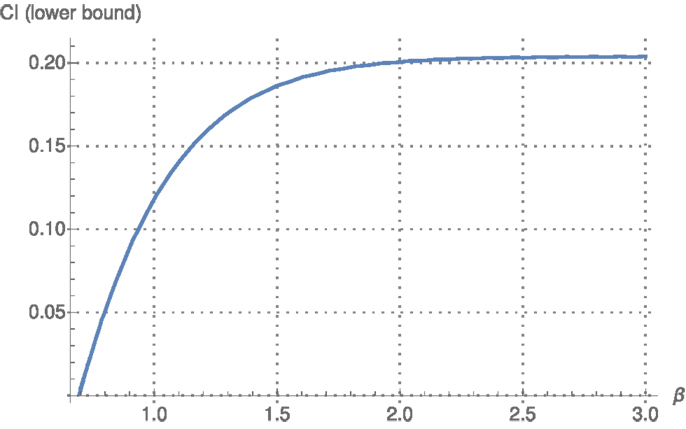
Figure 12. Lower bound for CI versus β. For each β ∈ [0.7, 3] we can find an α such that the joint p_α k_β lies in ∧. The increase in mutual information as β varies is a lower bound for CI, which is then in general non-zero.

We can see in Figure 11 that especially for very large or very small values of α and β (i.e., very strong or very weak correlation), CI captures the behavior of mutual information quite well. These limits are precisely deterministic and constant kernels, for which most approaches in quantifying synergy coincide. This is the reason why the examples studied in Griffith and Koch (2014) give quite a satisfying result for CI (in their notation, S_VK). For the less studied (and computationally more complex) intermediate values, like 1 < α, β < 2, the approximation is instead far from accurate, and in that interval (see Figure 12), there is a sharp increase in I, which leads to overestimating synergy.

6. Conclusion

Using information geometry, we have defined a non-negative decomposition of the mutual information between inputs and outputs of a channel.

The decomposition divides the mutual information into contributions of the different orders of synergy in a unique way. It does not, however, divide the mutual information into contributions of the different subsets of input nodes as Williams and Beer’s PID (Williams and Beer, 2010) would require.

For two inputs, our measure of synergy is closely related to the well-received quantification of synergy in Griffith and Koch (2014) and Bertschinger et al. (2014). Our measure though works in the desired way for an arbitrary (finite) number of inputs. Differently from Griffith and Koch (2014) and Bertschinger et al. (2014), anyway, we do not define a measure for redundant or “shared” information, nor unique information of the single inputs or subsets.

The decomposition depends on the choice of an input distribution. In case of input correlation, redundant information is counted automatically only once. This way, there is no need to quantify redundancy separately.

In general, there is no way to compute our quantities in closed form, but they can be approximated by an iterative-scaling algorithm (see, for example, Csiszár and Shields (2004)). The results are consistent with the intuitive properties of synergy, outlined in Williams and Beer (2010) and Griffith and Koch (2014).

Author Contributions

The research was initiated by NA. It was carried out by both authors, with main contribution by PP, who also wrote the article. Both authors read and approved the final manuscript.

Conflict of Interest Statement

The authors declare that the research was conducted in the absence of any commercial or financial relationships that could be construed as a potential conflict of interest. The handling editor Mikhail Prokopenko declares that despite having collaborated with author Nihat Ay, the review process was handled objectively and no conflict of interest exists.

Footnote

1. ^For an example in which I = 0 but the nodes are not independent, see Williams and Beer (2010).

References

Amari, S. (2001). Information geometry on a hierarchy of probability distributions. IEEE Trans. Inf. Theory 47, 1701–1709. doi: 10.1109/18.930911

CrossRef Full Text | Google Scholar

Amari, S., and Nagaoka, H. (2000). Methods of Information Geometry. Translations of Mathematical Monographs, vol. 191. Oxford: American Mathematical Society.

Google Scholar

Ay, N. (2015). Information geometry on complexity and stochastic interaction. Entropy 17, 2432. doi:10.3390/e17042432

CrossRef Full Text | Google Scholar

Bertschinger, N., Rauh, J., Olbrich, E., Jost, J., and Ay, N. (2014). Quantifying unique information. Entropy 16, 2161. doi:10.3390/e16042161

CrossRef Full Text | Google Scholar

Csiszár, I., and Shields, P. C. (2004). Information theory and statistics: a tutorial. Found. Trends Commun. Inf. Theory 1, 417–528. doi:10.1561/0100000004

CrossRef Full Text | Google Scholar

Griffith, V., and Koch, C. (2014). “Quantifying synergistic mutual information,” in Guided Self-Organization: Inception, Emergence, Complexity and Computation Series, vol. 9. Springer.

Google Scholar

Harder, M., Salge, C., and Polani, D. (2013). Bivariate measure of redundant information. Phys. Rev. E 87, 012130. doi:10.1103/PhysRevE.87.012130

PubMed Abstract | CrossRef Full Text | Google Scholar

Kakihara, Y. (1999). Abstract Methods in Information Theory. Series on Multivariant Analysis, vol. 4. Singapore: World Scientific.

Google Scholar

McGill, W. L. (1954). Multivariate information transmission. Psychometrika 19, 97–116. doi:10.1007/BF02289159

CrossRef Full Text | Google Scholar

Rauh, J., Bertschinger, N., Olbrich, E., and Jost, J. (2014). “Reconsidering unique information: towards a multivariate information decomposition,” in International Symposium on Information Theory (ISIT). IEEE.

Google Scholar

Schneidmann, E., Bialek, W., and Berry, M. J. II (2003a). Synergy, redundancy, and independence in population codes. J. Neurosci. 23, 11539–11553. doi:10.1523/JNEUROSCI.5319-04.2005

PubMed Abstract | CrossRef Full Text | Google Scholar

Schneidmann, E., Still, S., Berry, M. J. II, and Bialek, W. (2003b). Network information and connected correlations. Phys. Rev. Lett. 91, 238701–238704. doi:10.1103/PhysRevLett.91.238701

PubMed Abstract | CrossRef Full Text | Google Scholar

Williams, P. L. and Beer, R. D. (2010). Nonnegative decomposition of multivariate information. Preprint available on arXiv:1004.2151.

Google Scholar