Behavioral Diversity Generation in Autonomous Exploration through Reuse of Past Experience

1. Motivation

The engagement of robots and animals with the world generates a complex sensorimotor flow, which features a large motor space and multiple sensory modalities. While the body, as an active interface to the environment, simplifies in important ways the raw experience of the world (Hoffmann and Pfeifer, 2012), the learning and decision-making challenges the individual faces are still formidable.

In recent years, the child-as-a-scientist paradigm (Gopnik, 1997, 2012; Schulz and Bonawitz, 2007; Gweon and Schulz, 2008; Cook et al., 2011) has emerged as a major paradigm of child cognitive development. It considers the hypothesis that children can act as would rational thinkers, creating experiments and testing hypotheses through their interaction with the world in a manner structurally similar to scientific inquiry. Several works have indeed shown that preschoolers understand causality, distinguish it from spurious associations, and construct interventions to do so (Gopnik et al., 2001; Schulz et al., 2007).

Constructing and carrying out informative interventions, i.e., interactions that afford information gain, decrease the number of interactions necessary to understand a phenomenon, therefore ensuring an economy of time and energy. Yet, it also requires cognitive resources that may either be lacking (the individual cannot grasp the situation with his current cognitive abilities) or may represent too high an effort to justify the information gain they afford.

Robots – the focus of this paper – face a similar situation. In autonomous developmental contexts, robots do not have access to descriptions of their environments crafted by experts. Rather, they have to learn from experience. When social peers are not available, this experience has to be acquired autonomously from their own exploration of the environment. They have to act in unfamiliar situations that – due to a fundamental scarcity of knowledge – escape, at first, their abilities to fully grasp them, either through representation, prediction, control, or planning.

Designing informative interventions in those situations then faces a chicken-and-egg problem: knowing which interventions are going to be informative requires information that is not yet available, and that must be acquired through informative interventions.

Of course, that does not mean that informative interventions cannot be conducted, as any interaction can turn out to be informative a posteriori. But the fundamental problem of choosing which interventions to conduct while being unable to predict which ones are going to be informative remains.

A possible strategy, then, is to create behavioral diversity. Behavioral diversity characterizes the number and variety of behaviors an agent exhibits in its environment. Determining how different two behaviors are largely depends on the observer and its motives. For instance, a humanoid robot placed on a surface and executing random motor activations will engage in complex and unique patterns of movements and will end up convulsing on the floor most of the time. Arguably, each pattern of movement can be considered as a different behavior. But for a task such as standing up, the elevation of the head during movement might be the only relevant signal. In that perspective, all patterns of movement resulting in convulsions on the floor represent the same behavior while the robot sitting up or standing up represent different ones.

In this paper, and in the context of an autonomous robotic perspective, we characterize behaviors through the environmental feedback they elicit, as perceived by the robot itself, rather than the actions they necessitate. Exhibiting behavioral diversity then equates producing a diversity of effects in the environment. The dimensions of those define what we will call here, with three interchangeable terms: behavioral space, effect space, or sensory space.

Producing behavioral diversity can be a good strategy in unknown situations because it is not directed toward – and as such not constrained to produce information about – a specific goal. Instead, it creates a set of observations about diverse features of the environment, offering the robot a set of options that can be explored and exploited toward specific objectives afterward. The usefulness of such strategies for robots has been recently explored through models of curiosity-driven learning and intrinsically motivated reinforcement learning (Oudeyer and Kaplan, 2007; Baldassarre and Mirolli, 2013; Benureau and Oudeyer, 2015), and in a related line of work, on novelty and diversity search in evolutionary robotics (Mouret and Doncieux, 2009; Lehman and Stanley, 2011).

In many practical contexts, the situation facing the robot is not completely unknown, and rational deductions and inferences can be made about what type of interactions are going to be informative. Still, they may not narrow the number of candidate interventions to a reasonable number. In that context, producing behavioral diversity can be seen as an essential strategy to deal with the limits of pure logical reasoning. It provides a heuristic mechanism for discovering knowledge by the learner-as-a-scientist (be it a human or a robot) when rational mechanisms used to uncover the laws of the world cannot be applied.

In other words, such a heuristic picks up when rational deductions end: logical reasoning identifies a set of interactions worth trying, and the behavioral diversity heuristic provides a sampling method to choose what to try among this remaining set. For instance, a child playing with a teddy bear and a rattle may understand that to figure out what a rattle does, interactions with the teddy bear are uninformative. This halves the space of candidate interactions but provides no clue about which interactions are interesting to try on the rattle. Trying to interact with the rattle in different ways is then an effective strategy.

This selective exploration principle is elegantly formulated by Cook et al. (2011) in the children’s case: “selective exploration of confounded evidence is advantageous even if children explore randomly (with no understanding of how to isolate variables): the more different actions children perform, the better their odds of generating informative data.” (p. 352). Gweon and Schulz (2008) provide a study where children presented with confounding evidence increase the variability of their exploration, even if that represents a physical effort. Schulz and Bonawitz (2007) and Bonawitz et al. (2012) report similar results: children preferentially engage with a confounding toy, rather than to play with a new one.

But producing behavioral diversity is not necessarily a trivial task. While producing random motor behavior is algorithmically straightforward – it boils down to picking a random motor action among the ones available – it does not typically generate a diversity of interactions and effects in the environment: motor diversity does not translate into effect diversity. This is caused by the typical heterogeneous distribution of the redundancy of the sensorimotor space: to some effects correspond a large number of motor commands, while some effects can only be produced by a small, specific set of them. In an interaction task with an object, for instance, few motor commands may actually produce contact with the object. The rest of them produce the same effect on the object: nothing. As such, a uniform, random sampling of a large motor space will only produce effects in highly redundant parts of the sensory space for any reasonable (i.e., at the timescale of a lifetime) number of samples. Therefore, an efficient sampling strategy must be devised.

However, as producing behavioral diversity is most useful in tasks where little or no knowledge of the underlying environmental mechanisms exists, and this knowledge is precisely what would be needed to choose which interactions to carry in order to produce effects as diverse as possible, the production of behavioral diversity suffers a similar chicken-and-egg problem as the one raised by the design of informative interventions: it needs knowledge to create interactions that will generate data that will serve to derive the knowledge it needs.

One possibility to break the circularity is to procure knowledge from somewhere else. In this paper, we introduce a method to create behavioral diversity in an unknown task by leveraging past experience from another task. We consider a scenario where one task has been explored, and a new, unknown task is presented to the robot. The relationship between the two tasks is not given to the robot, and can be arbitrary. The only constraint is that at least some motor commands executed in the previous task can be reexecuted in the new one. Besides this, the method transparently adapts to arbitrary changes in sensory modalities and learning algorithms between tasks.

In the next section, we first formalize the problem (Section 2) and introduce a measure to quantify behavioral diversity in continuous sensorimotor spaces. We then introduce our method (Section 3). In Section 4, we present a simple application of the method. Then, in Section 5, we detail a more complex situation where a robotic arm interacts with different objects.

2. Problem

An environment is here formally defined as a mapping f from M to S, which can be stochastic. M is the motor space, and it represents a parameterization of the movements the robot can execute. It is a bounded hyperrectangle of ${\mathbb{R}}^{d_M}$; d_M is the dimension of the motor space. S is the effect space, of dimension d_S; it is a bounded subset of ${\mathbb{R}}^{d_S}$. Effects and goals (i.e., desired effects) are elements of S. In this paper, both M and S are multidimensional continuous spaces, with d_S ≪ d_M.

Here, the elements of the motor space do not directly encode the raw commands that the motors of the robot receive. Instead, we use motor primitives that transform vectors of parameters from the motor space M into streams of real-time, hardware-specific motor commands. A motor primitive can be a simple goal position for a given motor, or be a Dynamic Movement Primitive (DMP) (Ijspeert et al., 2013) that translates parameters into smooth motor trajectories; both will be used in this paper. Likewise, the sensory space does not contain the raw readings of the sensors but rather behavioral descriptors: parameterized behavioral representations of raw sensors data after it has been processed by sensory primitives. Concretely, a sensory primitive can encode the position of an end-effector in Cartesian space or the displacement of an object after a robot interacted with it. This allows to flexibly encode sensory feedback into high-level representations. Such sensory primitives do not only abstract low-level feedback data: they represent the robot’s attention, by encoding specific features of the environment and not others, and we use them deliberately this way in this paper.

Environments are black boxes, and only the parameterizations M and S are known to the robot. Let us remark that, while valuable information can be encoded in the boundaries of S, nothing prevents S to be arbitrarily large compared to the reachable space f (M), i.e., the set of effects that can actually be produced. In order to avoid unnecessary complexity in this paper, we will only consider experiments where S is not significantly larger than the axis-aligned bounding box of f (M). A method to deal with arbitrarily large S can be found in Benureau and Oudeyer (2015).

An exploration task, subsequently referred simply as a task, is defined as a pair (f, n) with f: M ↦ S the environment and n the maximum number of samples of f allowed, i.e., the number of actions the robot can execute in the environment.

We will consider scenarios made of two tasks, a task A = ( f_A, n_A), the source task, and a task B = ( f_B, n_B), the target task. We assume that motor commands from M_A can be reexecuted in the target task. In this paper, we will consider M_A = M_B, but other scenarios are possible, such as the existence of a known mapping between the two motor spaces (for instance, reusing motor commands used on the left arm of a humanoid on its right one). The reexecutability constraint is a strong one, but as robots body typically change much less quickly than their environments, many tasks share the same motor space. This may be less true for high-level motor, or action, spaces, but if no known mapping exists for the action spaces of two different tasks, the method does not just faces a problem of applicability: it is also probably of little use.

The source task is considered to have been interacted with using an arbitrary method, generating a sequence of observations ${\left\{{\mathbf{x}}_i,{\mathbf{y}}_i\right\}}_{0\le i<n_A}$ in ${\left(M_A\times S_A\right)}^{n_A}$, composed of the executed motor commands and observed effects. On the other hand, the robot has not yet interacted with the target task B.

The problem we are tackling in this paper is the question of transfer: how can the previous interaction with task A can be exploited to improve the exploration of task B?

We compare the case where information from A is exploited versus the situation where it is not, using as a baseline mechanism a random goal babbling architecture (SAGG-Random). Goal babbling has previously been shown to be an efficient strategy for the acquisition of inverse models (Baranes and Oudeyer, 2013; Moulin-Frier and Oudeyer, 2013) and in the production of behavioral diversity. We compare both cases using a behavioral diversity measure: threshold coverage (Benureau and Oudeyer, 2015). Improving the exploration of task B therefore means increasing the threshold coverage.

2.1. Threshold Coverage

Threshold coverage or τ-coverage is a behavioral diversity measure: it considers only the consequences of the motor commands, i.e., in our autonomous context, the behavioral effects as encoded in S, not the motor activations themselves. Motor motions can of course be part of behavior and contribute to diversity, when adequate sensors and sensory primitives are used to encode them in S. This is, for instance, the case in the behavioral descriptors used by the MAP-Elites algorithms (Cully et al., 2015).

Threshold coverage considers the volume of the union of the set of hyperballs of radius τ – the threshold – that have for centers the observed effects (Figure 1).

FIGURE 1

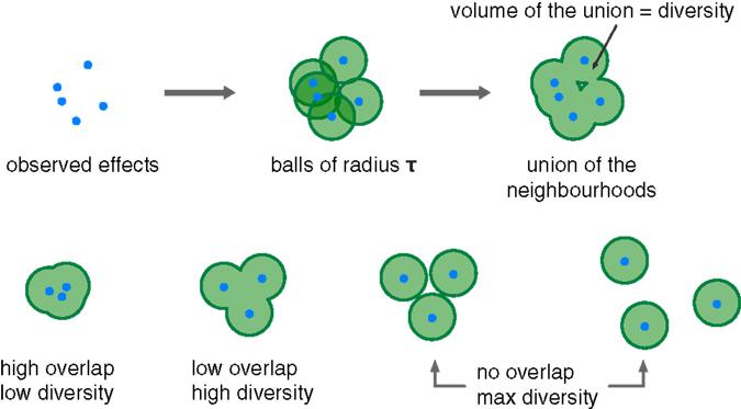
Figure 1. In this 2D example, the threshold diversity is represented by the green area (top). The threshold diversity measure quantifies how spread are the observed effects, up to a threshold τ. The measure is not sensitive to differences between distributions where all centers are pairwise more distant than τ (bottom).

Formally, considering a set of points C belonging to ℝⁿ, and τ ∈ ℝ⁺, we define the τ-coverage of C as:

${\text{coverage}}_{\mathrm{\tau }}\left(C\right)=\text{volume}\left({\displaystyle \bigcup _{{\mathbf{y}}_i\in C}}B\left({\mathbf{y}}_i,\mathrm{\tau }\right)\right)$

with B(y_i, τ) the hyperball of center y_i and radius τ.

The threshold coverage measure allows to quantify how much of the effect space is not more distant than τ of an observed effect. As a consequence, the threshold coverage measure is insensitive to differences between sets where the observed effects are pairwise more distant than τ (Figure 1).

Computing the threshold coverage requires to compute the volume of an arbitrary set of balls of the same radius. Exact methods exist using Voronoi Power Diagrams (Cazals et al., 2011), that partition the space into as many areas as there are balls; in each area, the center of only one ball is present, and the contribution of this ball to the overall volume can be computed independently of the others. There are also approximate methods based on Monte-Carlo sampling (Till and Ullmann, 2009).

We use the threshold coverage to characterize and contrast the robots’ behavior under different algorithms. Let us remark that the robot, as an autonomous agent, never has access to the threshold coverage measure; it is purely an experimenter’s tool.

3. Method

The idea behind our algorithm is to select a subset of motor commands executed during the exploration of the source task, and reexecute each of them on the target task. This subset is assembled with motor commands that generated diverse effects, i.e., that generated behavioral diversity, in the source task.

The assumption is that the production of behavioral diversity is due to the motor commands generating forces that engage the environment in different ways. Reexecuted in a different task, these motor commands are a priori more likely to generate a diverse set of effects – and thus information – than a set of motor commands that produced the same effect in the source task.

We can interpret the method in the context of the learner-as-a-scientist paradigm; it can be viewed as creating a repertoire of experiments to conduct in unknown situations to discover how the environment behaves and what interactions it responds to. This type of behavior is seen in nature: “A young corvide bird, confronted with an object it has never seen, runs through practically all of its behavioral patterns, except social and sexual ones” (Lorenz, 1996).

Likewise, a robot interacting with a ball needs to use different movements to make it roll left, right or forward. Having learned those movements, if the robot is provided with a cube, the prediction or control model of the ball is difficult to exploit directly: the two objects have significantly different dynamics. However, by reusing the behavioral patterns – the movements – on the cube that pushed the ball in different directions, the robot can immediately produce a diversity of effects on the cube, and start learning which ones still apply and are most effective.

Selecting motor commands through diversity can be understood as trying to filter body redundancy. In a given task, the redundancy of the body and the environment will make different motor commands produce the same effect, as Figure 2 illustrates. If the body redundancy is at play, two different motor commands will end up applying similar forces on the environment: this is the case of a redundant multi-joint robotic arm, where multiple motor motions exist that generate the same end-effector trajectory. If the environmental redundancy is at play, different forces will produce the same salient effect: this is the case when pushing or pulling on a closed door. A set of motor commands that produce a diversity of effects tends to display neither body nor environmental redundancy. When the environment changes, the absence of body redundancy is conserved among this set. And if the new environment is similar to the old one, some of the environmental redundancy may be avoided as well.

FIGURE 2

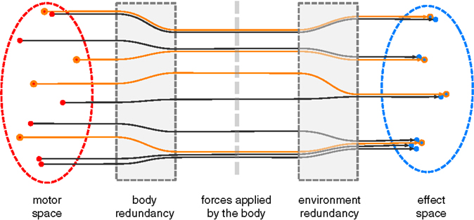
Figure 2. In this schematic representation, four clusters of effects are produced through different types of redundancies. From top to bottom, the first two effects are similar because their motor commands are similar. The second cluster exhibits body redundancy: two different motor commands end up generating the same forces on the environment. The third exhibits environmental redundancy: different forces produce the same effect. The fourth exhibits all of the three previous cases. Assuming the environment is neither stochastic nor chaotic, when selecting a diverse set of effects in the sensory space (for instance, the set highlighted in orange), the set of motor commands that generated them tends to display low body redundancy.

Of course, a stochastic or chaotic environment can counterbalance its redundancy: the same motor command executed multiple times can generate diverse effects. In that case, however, reexecuting this motor command multiple times in the new task is a justified strategy to generate diversity.

In the following, we detail first how the source task is explored, and the learning algorithms we use. Then, we explain how the exploration is modified for the target task.

3.1. Exploration of the Source Task

In this paper, the source task will be explored using a goal-directed exploration algorithm. Goal-directed exploration (Oudeyer and Kaplan, 2007) implementations have been proposed in Baranes and Oudeyer (2010), Jamone et al. (2011), and Rolf et al. (2011), and as part of the SAGG-RIAC architecture (Baranes and Oudeyer, 2013) and have been shown to be effective in exploring sensorimotor spaces with large motor spaces. These methods for goal babbling as well as related methods such as MAP-Elite (Cully et al., 2015) have also been shown to efficiently generate forms of behavioral diversity.

In what follows, we introduce and use the Explore algorithm, a variant of the SAGG-Random goal babbling algorithmic architecture (Baranes and Oudeyer, 2013; Moulin-Frier and Oudeyer, 2013). We adapt SAGG-Random by adding a bootstrapping phase of random motor babbling lasting K_boot steps before the random goal babbling phase (Algorithm 1); the bootstrapping phase is necessary because the inverse models we use need some existing data to work. During the bootstrapping phase, random motor commands are executed, while during the random goal babbling phase, random goals are chosen uniformly in S, and an inverse model (introduced in Section 3.2) is used to transform goals into motor commands. In the experiments, we set K_boot to a low value in order to reduce the duration of the random motor babbling phase, without significantly compromising performance. In a more general context, K_boot could be computed dynamically, for instance, by using the method introduced in Benureau and Oudeyer (2015).

ALGORITHM 1

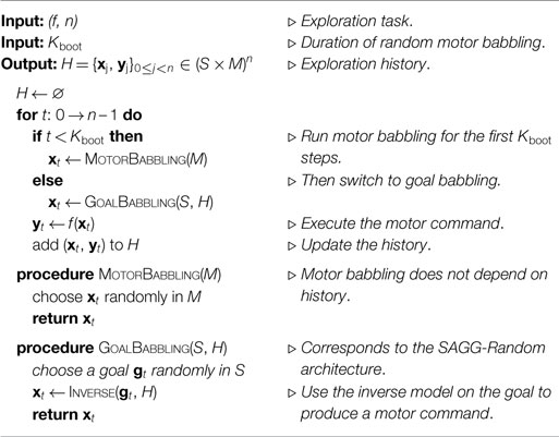
Algorithm 1. Expolore ((f, n), K_boot).

We use here two implementations of this architecture, corresponding to two different learning algorithms, InversePerturb and InverseLBFGSB-LWLR, to implement the Inverse step, as described in the next section.

3.2. Inverse Model

An inverse model is used whenever goal babbling is chosen as an exploration strategy in the Explore algorithm. Let us remark that our objective here is not to acquire a forward or inverse model of the environment. The learning algorithms are functional entities of the exploration process, and the models they produce are not evaluated. In particular, they may make assumptions that preclude them from creating accurate models of the environment – we will discuss such a case in Section 4. In this article, we will be using two different inverse models: a simple, perturbation-based one and another based on an optimized regression method.

3.2.1. Perturbation-Based Inverse Model

The perturbation-based model finds the best motor command to reach the goal among those already executed in the past and creates a slightly perturbed variation of it to be executed, in a fashion similar to the mutation operators of evolutionary algorithms.

Given a motor command $\mathbf{x}=\left\{x_0,x_1,\dots ,x_{d_M-1}\right\}$ in M, a perturbation of x is defined by:

${\text{P}\mathrm{ERTURB}}_d\left(\mathbf{x}\right)=\{\text{R}\mathrm{ANDOM}\left(\text{max}\left(a_i,x_i-d\left(b_i-a_i\right)\right),\text{min}\left(x_i+d\left(b_i-a_i\right),b_i\right)\right){\}}_{0\le i<d_M}$

with $M={\prod }_{0\le i<d_M}\left[a_i,b_i\right]$ as a hyperrectangle of ${\mathbb{R}}^{d_M}$ and with the function Random(a,b) drawing a random value in the interval [a,b] according to a uniform distribution. d is the perturbation parameter, and belongs to [0, 1]; it is the only parameter of the inverse model, that we can now express in Algorithm 2.

ALGORITHM 2

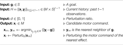
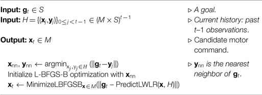
Algorithm 2. InversePerturb_d(g_t, H).

This perturbation-based inverse algorithm is simple and effective. Its complexity is linear in both d_M (perturbation) and nd_s (nearest neighbor search). Its main assumption is that a small perturbation of the motor space produces a comparatively small change in the sensory feedback. The model has difficulties escaping local minima. In practice, in the experimental contexts considered in this paper, the performance and robustness of this model is competitive with more complex approaches. This inverse model is not completely unreasonable in biological organisms (Loeb, 2012), and that related algorithms implemented as part of the SAGG-Random architecture such as in Baranes and Oudeyer (2013) and Moulin-Frier et al. (2014), as well as other variations such as the MAP-Elite algorithm (Cully et al., 2015), have yielded good results in diverse robotics contexts.

3.2.2. Optimized Regression Inverse Model

We also use an optimized regression inverse model in some experiments, based on an optimization routine, L-BFGS-B (Byrd et al., 1995; Zhu et al., 1997), and a predictor, Locally Weighted Linear Regression (LWLR) (Cleveland and Devlin, 1988; Atkeson et al., 1997a,b).

3.2.2.1. Forward Model

To approximate the function f from a set of observations, we employ Locally Weighted Linear Regression (LWLR) (Cleveland and Devlin, 1988; Atkeson et al., 1997a,b), an incremental machine learning algorithm. Although LWLR is more sophisticated than the perturbation-based inverse model, it is still a simple method compared to the state-of-the-art. Here, the absolute learning performance is of little concern as we are interested in comparing different exploration strategies. Still, LWLR is reasonably robust (Munzer et al., 2014) for the learning tasks we are considering. Compared to the perturbation-based inverse model, LWLR is able to extrapolate, i.e., the distance between the goal and the existing observations is taken into account, but it also needs several closely clustered observations to do so efficiently; the perturbation-based inverse model only ever needs one.

Given a set of observations H = {(x_j,y_j)}_0≤j<t–1 where for each j, f (x_j) = y_j, and given a query vector x_q, for which we wish to predict the effect, we compute the Euclidean distance to x_q from each point x_j, and derive the following Gaussian weights w_j:

$w_j=e^{\frac{-{\parallel {\mathbf{x}}_j-{\mathbf{x}}_q\parallel }^2}{2{\mathrm{\sigma }}^2}}$

We consider the matrices X with X_i,j = (x_i)_j, Y with Y_i,j = (y_i)_j, and W = diag(w₀,w₁,…w_t–2), and compute:

$\mathrm{\beta }={\left({\left(\mathit{WX}\right)}^T\mathit{WX}\right)}^{+}\left({\left(\mathit{WX}\right)}^T\mathit{WY}\right)$

where (WX)^TWX is a symmetric matrix, and ((WX)^TWX)⁺ is its Moore–Penrose inverse (Penrose and Todd, 1955). Then,

${\mathbf{y}}_q={\mathbf{x}}_q\mathrm{\beta }$

y_q is the LWLR estimate of x_q, given the observed data H. We call PredictLWLR(x_q, H) the function that computes y_q for any x_q ∈ M given H.

In our implementation, σ, which controls the locality of the regression, is dynamically computed. We compute σ as the average distance of the k = 2d_M + 1 closest points of the query vector x_q. All other points of H besides the k closest neighbors are given a weight of zero.

3.2.2.2. Inverse Model

Given a goal g_t ∈ S, we want to produce a motor command x_t ∈ M so that || f (x_t) – g_t|| is small.

With M being a hyperrectangle of ℝ^d_M, we use L-BFGS-B (Limited-memory Broyden–Fletcher–Goldfarb–Shanno Bound constrained (Byrd et al., 1995; Zhu et al., 1997), version 3.0 (Morales and Nocedal, 2011)), a quasi-Newton method for bound-constrained optimization, to minimize the error. L-BFGS-B use an approximation of the Hessian matrix to direct the optimization (because the Hessian cannot be directly computed, it is approximated using finite differences). We approximate ||f (x) – g|| with ||PredictLWLR(x, H) – g|| and use it with L-BFGS-B to further approximate argmin_x∈M(||f (x) – g||).

The optimization process is initialized with the motor command corresponding to the closest neighbor of g in the set of observations (see Algorithm 3).

ALGORITHM 3

Algorithm 3. InverseLBFGSB-LWLR(g_t, H).

The Inverse method is replaced by either InversePerturb or InverseLBFGSB-LWLR in the source task exploration algorithm, Explore, and the one of the target task, Reuse, that we introduce now.

3.3. Exploration of the Target Task

The exploration of the target task is organized around two algorithms. The first, Transfer, is applied at the end of the interaction with the source task and produce a set of motor commands bins that are used by the second, Reuse, to affect the exploration of the target task.

The Transfer selects motor commands that produced a diversity of effects. It works by partitioning the sensory space of the source task, S_A. We use a simple grid here. To each cell of the grid corresponds a bin of motor commands that contains all the motor commands whose effects belong to the cell. This way, similar effects in the source task have their motor command gathered in the same bin (see Algorithm 4).

ALGORITHM 4

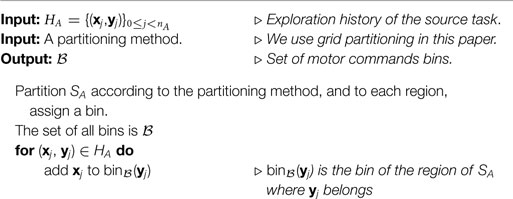
Algorithm 4. Transfer(H_A).

The Reuse method is a variation of the Explore algorithm, where a part of the random motor babbling steps are replaced by reuse steps. During a reuse step, a random bin among the ones generated by the Transfer algorithm is selected, and a random motor command is drawn from the bin without replacement and executed in the environment. Such a selection generates a sequence of motor commands that correspond to effects representative, on average, of the diversity of effects produced in the source task. Goal babbling behavior is unaffected.

To produce the Reuse method, the call to MotorBabbling in the Explore algorithm is replaced by a probabilistic call to ReuseBabbling and MotorBabbling, according to a probability p_reuse (see Algorithm 5).

ALGORITHM 5

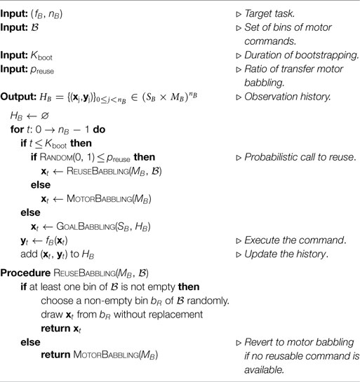
Algorithm 5. Reuse((f_B, n_B), ℬ, K_boot, p_reuse).

This procedure has a low computational cost, and only transfers structured sets of motor commands between tasks. No sensory data are shared across tasks, which mean that no forward or inverse model is shared. It makes the method compatible with arbitrary changes in sensory modalities, and insensitive to the quality forward or inverse models of the source task, should they exist. Furthermore, by separating the Transfer and Reuse method, we can precompute the transferred data before the second task is known, and then use it even if the sensory data of the first task has been forgotten.

Here, we have proposed a Transfer method that partitions the sensory space of the source task. This partitioning encodes diversity, and may be non-trivial in complex sensory spaces. There is flexibility in how the Transfer method could be implemented however. It could, through an arbitrary method – optimization of a diversity measure for instance – build a small set of motor commands whose effects have high diversity, and return a single bin containing them to the Reuse method, discarding other observations from the source task. The Reuse method would select randomly from this single bin as a result.

In the following sections, we conduct experiments to show that Reuse is effective in situations that involve changes in the morphology of the robot (arms with different link lengths in Section 4), that involve switching an object for another between the source and the target task (ball/cube experiment in Section 5.2), exploiting pure random motor babbling (Section 5.2.2), dealing with dissimilar situations (Section 5.2.3), and scaffolding ones (pool experiment in Section 5.3). We also investigate how Reuse can be used to exploit simulation results on real robots (Section 5.5).

4. Experiment on Planar Arms

To illustrate the Reuse method, let us consider a pair of planar robotic arms, each with 20 joints. The first arm has same-length links totaling one meter, and the environment returns the Cartesian position of the end-effector. The second arm has links such that, going from the base to the end-effector, each link is 0.9 times smaller than the previous one, while the total length of the arm remains one meter; this arm also returns the position of the end-effector, but using polar coordinates (Figure 3).¹

FIGURE 3

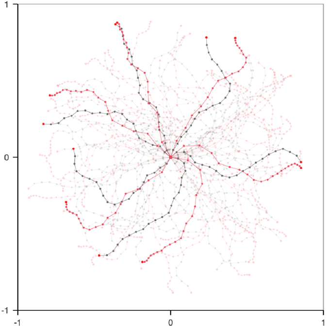
Figure 3. When executing the same command on both arms, the position of the end-effector is significantly different most of the time. Here depicted are 50 pairs of executions of the same motor command on the two 20-joint arms, five of which that are highlighted.

The two arms have a different morphology – a situation akin to morphological development. They share, however, the same number of joints with the same available ranges (±150°): they have the same motor space and motor parameterization. However, because the lengths of the links are different, most motor commands will result in a different position for the end-effector, as shown in Figure 3. And because the positions are expressed in two different coordinate systems, the inverse model of one arm is difficult to exploit on the other arm, without having, or learning, a mapping between the coordinate systems.

The exploration on the first arm is conducted over 5000 steps, using the Explore algorithm with K_boot = 50, with the perturbation-based inverse model with d = 0.05, i.e., perturbing each joint by at most ± 15°.

The exploration of the target arm is the same as the source arm, except that all the 50 motor babbling steps of the source exploration strategy are replaced by reuse steps, as per the Reuse algorithm with p_reuse = 1. Figure 4A illustrates how motor commands to be reused are selected, as per the Transfer algorithm. Figures 4B,C show the difference between the bootstrapping phase of the Reuse and Explore algorithm. The impact of Reuse on the exploration is important at the beginning and remains beneficial throughout, even after 5000 steps.

FIGURE 4

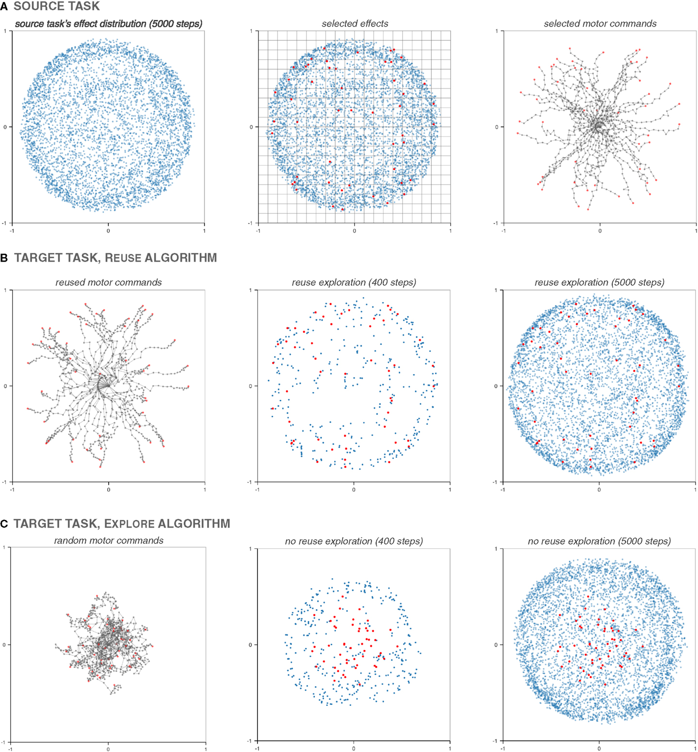
Figure 4. Illustration of the Reuse algorithm. After the end of the exploration of the source arm (A), a 20 × 20 grid partitions the effect space, and as many times as necessary (50 times here), a random cell is chosen, as well as a random effect inside it (dots highlighted in red). The motor commands that produced the chosen effects are then reexecuted on the target arm (B). This replaces the initial 50 motor babbling steps of the Explore algorithm (C). In both cases, the effects produced by random motor babbling or a reused motor command have been highlighted in red. While random motor babbling produces convoluted arm postures whose effects are clustered around the center, the reused motor commands produce effects spread out over the reachable space, and feature straighter postures. This difference in bootstrapping has a huge impact on the coverage at t = 400, and a lesser, but still present one after 5000 steps.

Figure 5 displays the τ-coverage (with τ = 0.05) of both the Reuse and the Explore algorithm on the target arm over 100 repetitions of the experiment. In both cases, the coverage was computed in the Euclidean space. The Reuse strategy provides a performance increase that last even after 5000 steps: in 75% of the cases, the Reuse strategy performs strictly better than the best-case scenario of the Explore strategy. The usage of Reuse accelerates the exploration of the reachable space.

FIGURE 5

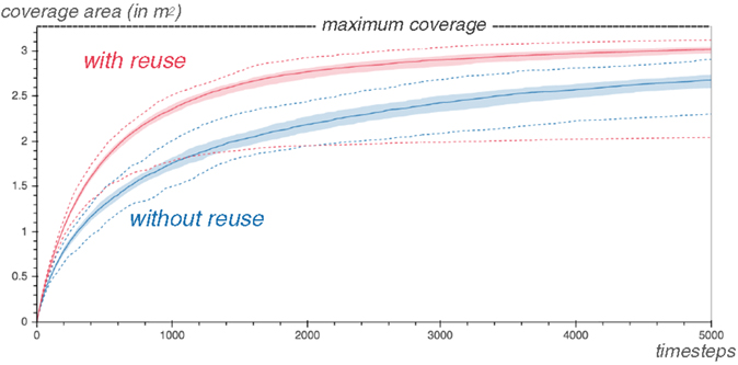
Figure 5. The exploration with Reuse on the second arm covers significantly more of the reachable space early on than the one without. The graph shows the τ-coverage (with τ = 0.05) of the second arm explored with the Reuse and Explore algorithm respectively, over 100 repetitions of each experiment. The median case is displayed, surrounded by a margin going from the 25th to the 75th percentiles. In dashed lines, the worst and the best coverages are also pictured.

However, an interesting phenomenon is present. The worst case of the Reuse strategy, as shown by the dotted lines, performs worse than the worst case of the Explore strategy.

To understand why, it is interesting to look at goal babbling as an evolutionary algorithm. From an evolutionary robotics perspective, the motor commands are the genetic encoding, the arm posture the phenotype and the effect – the position of the end effector – is the behavior of the arm. At each timestep of goal babbling, a random goal is chosen. The distance to this goal defines a fitness function, and the highest-performing past observation, whose effect is the nearest neighbor of the goal, is chosen to reproduce through mutation: this is how our perturbation-based inverse model works.

Therefore, after the bootstrapping phase, arm postures are chosen for reproduction in proportion of how close their effects are to the chosen goals. When using random motor babbling, most postures produce effects near the center. Because goals are randomly chosen in the [−1,1] × [−1,1] square, most goals are farther from the center than most observed effects. It means that postures producing effects on the edge of the initial cluster are chosen and mutated with disproportionate frequency. Through repeated selection and mutations those postures and their descendants, straighter and straighter postures are discovered.

Sometimes, however, those initial arm postures contain loops. Those loops represent local minima that are difficult to escape. The mutation and selection process – our perturbation-based inverse model – tends to straighten arm postures to reach distant target. In the process, loops are tightened, not removed. Therefore, the maximum span of the arm is reduced, and the exploration covers only a fraction of the reachable space, as shown in the graphs of Figure 6.

FIGURE 6

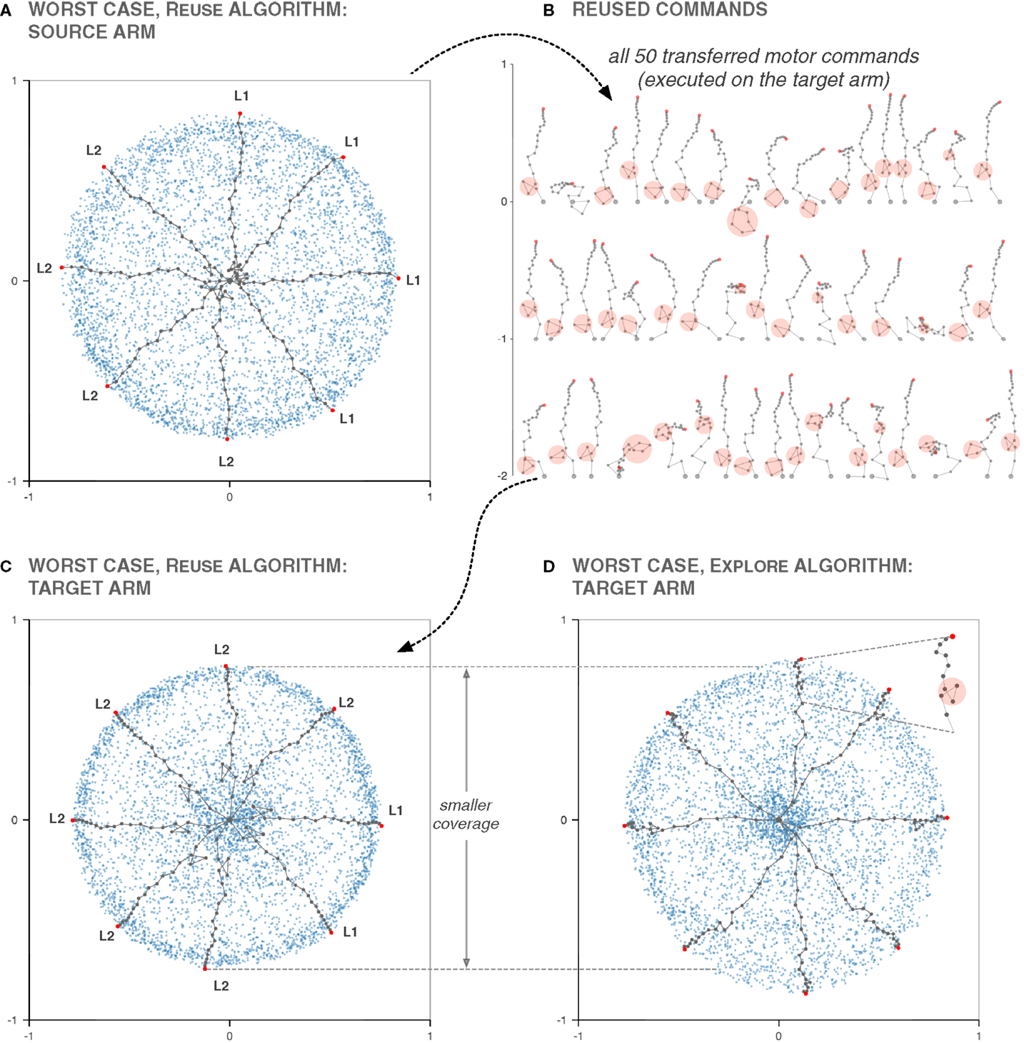
Figure 6. Using Reuse can be worse than not using it. This graphs depicts the worst case – coverage-wise – of the Reuse and Explore algorithms among the 100 cases used to compute Figure 5, for t = 5000. In (A,C,D), the arm postures with the longest span in the cardinal and intercardinal directions are displayed. In the worst case of Reuse, the source exploration features postures that have loops near the base of the arm (A). We can even distinguish between two species of postures. Ones that have a loop starting on the first joint (L1), and ones on the second joint (L2). Those postures are selected by the Reuse algorithm (B), and reexecuted in the target task (C), resulting in posture with loops that severely limits the span of the arm, as they are composed of long segments. The species distribution L1/L2 is remarkably similar between the source and the target task. When Explore is run directly on the target arm, those loops are eliminated by the competition with posture without loops or with loops near the tip of the arm, of far less consequence.

On the source arm, because the links are all of the same length, loops have the same cost in span regardless of where they appear. But on the target arm, they are most costly near the base of the arm, where links are longer. Therefore, arm postures featuring loops near the base of the arm tend to be shorter on average than postures with loops near the tip, even in a random motor babbling sampling. It means that, when using the Explore algorithm, most of the time, those postures do not get selected for far goals after the bootstrapping phase, as better solutions exist. Therefore, the postures that explore the edge of the reachable space have a tendency to have either loops near the tip of the arm or no loops at all.

The only way for postures with costly loops near the base of the arm to be selected on the target arm is for them to have the rest of the arm rather straight, and in a fashion disproportionate with the other arm postures they compete with. This is exactly the scenario that happens in the worst case of Reuse: all the reused arm postures where the tip is far from the center have loops near the base of the arm, as Figure 6 illustrates. This is not a problem for the source arm, but for the target arm it limits the achievable span much more than if the loops were near the tip of the arm.

This explains the difference in coverage between the worst case of the Reuse and Explore algorithm on the target arm, and serves to illustrate a danger of the Reuse algorithm: providing good solutions trapped in local minima early in exploration can prevent the discovery of better solutions, more adapted to the target task. Let us remark here that all the 50 motor babbling steps of the Explore algorithm were replaced by reuse steps in the Reuse algorithm. But allowing a portion of the 50 steps to remain random motor babbling, for instance with p_reuse = 0.5, would not solve the problem (we tested), as the arm postures with the best span in the bootstrapping phase would remain the reused ones, and get selected and mutated more than the others.

Of course, the occurrence of such a problem is highly contingent on the specifics of the two tasks, on how goals are chosen and what inverse model is used. But the risk, when transferring knowledge or skill from one task to another, to negatively impact the performance in the target task is always a possibility, and is difficult to protect from inside the framework of the problem we are considering.

Still, this does not mean that Reuse should be avoided. While it has the potential to induce performance-hindering local minima, it also has the potential to propose good solutions early in exploration. During the first 150 steps, the worst case scenario of the Reuse algorithm is actually better than the best-case scenario of the Explore one. In a robotic and operational context, having good-enough solutions quickly might matter more than finding perfect ones eventually. Robots do not live at the asymptote. If a robot needs to learn how to whisk for a recipe, it may matter more than the eggs and milk are mixed under 15 minutes than the fact that the quickly discovered whisking motion consumes more energy, is less efficient and makes more noise than necessary. Even in a learning context, having good early performance can help decide quickly if the skill is possible to learn, worth learning, and can help form an estimation of what is achievable in the target task, which may in turn quickly bootstrap planning capabilities.

Before moving on to a more complex experimental setup, it is interesting to analyze why the Reuse method is effective. As pointed out before, the two arms have different inverse models, and the relationship between them is non-trivial. By reusing motor commands that produce a diversity of effects, we make the assumption that the diversity mapping is simpler between the two tasks: a set of motor commands generating a certain amount of diversity on the source arm will generate a similar amount on the target arm. This is something we can verify experimentally.

In Figure 7, the coverage of sets of random motor commands of diverse sizes is highly correlated between the two arms. This correlation in the production of diversity is therefore an assumption it seems possible to rely on and exploit, even, in some cases, when the sensory modalities or the morphology of the robots are different between tasks.

FIGURE 7

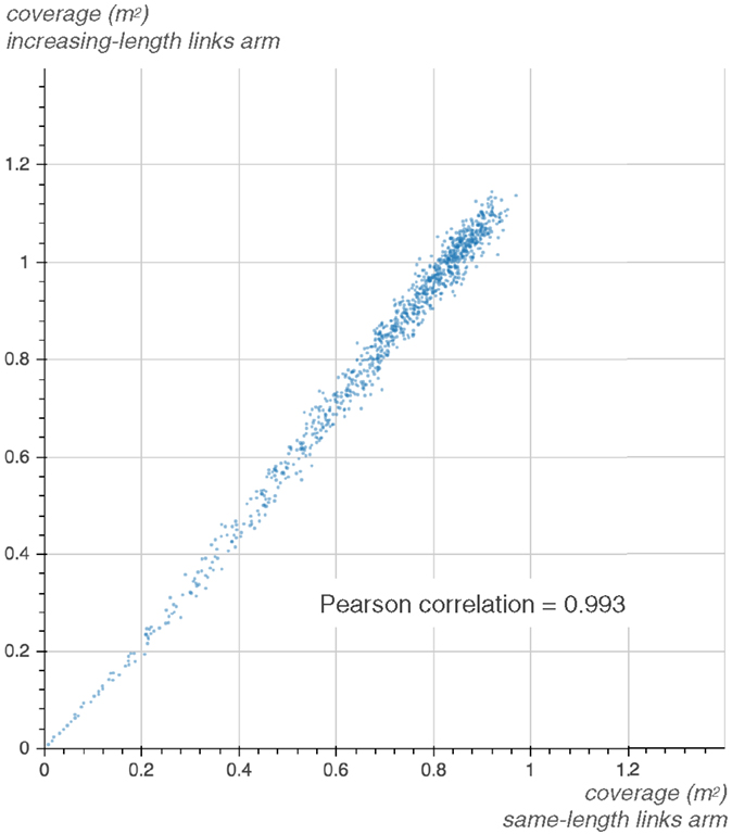
Figure 7. The diversity production of the same-length-links arm and the increasing-length-links arm is highly correlated. The graph displays the coverage of 1000 different sets of random motor commands of size 1, 2, …, 1000, respectively, for the 20-joint source and target arm, with τ = 0.05.

5. Object Interaction Tasks

5.1. Experimental Setup

We consider an experiment where a robotic arm interacts with an object and observes its displacement at the end of the interaction. In a developmental context, an interaction task is relevant, as it pertains to the early exploration of the world, where the function of most objects is still unknown.

We used both a simulated and a hardware setup, but comparatively few experiments were conducted on the hardware. For this reason, in this section, we mainly focus on describing the simulated setup, but discuss aspects related to the morphology of the real robot as well. The hardware setup is thoroughly described in Section 5.4.

The robot is a serial chain of six servomotors. The three proximal motors are Dynamixel RX-64 and the three distal ones are RX-28. Those servomotors are capable of delivering respectively 6.0 and 2.5 N ⋅ m of stall torque, with an angular resolution of 0.29°, measured with a mechanical potentiometer, whose precision is variable (across the angle range and between different motors). During the experiments, the real servomotors were operated in position control mode using the embedded PIDs, with a control loop for the position running at 100 Hz. In simulation, the physical characteristics of the motors are reproduced as much as possible, and their control in position is done in lockstep with the physics engine simulation steps, at 50 Hz.

5.1.1. Dynamic Movement Primitives

The movements of the robot are generated using dynamic movement primitives (DMP). DMPs are parametrized dynamical systems introduced by Ijspeert et al. (2002). They are computed from sets of differential equations that produce smooth movements robust to perturbations. We chose DMPs, and the specific parameterization we explain below, because it allowed to express many different arm trajectories with a compact description (i.e., few motor dimensions). We use the implementation of Stulp (2014), based on Ijspeert et al. (2013) with the sigmoid variation of Kulvicius et al. (2012).

DMPs are based on damped spring dynamics, perturbed by a forcing term [equation (1)]. The forcing term is a linear combination of basis functions [equation (4)]. Here, Gaussian activation functions ψ_i(s_t) are used, with center c_i and width σ_i, weighted by w_i [equation (3)]. v_t is the phase of the forcing term, described by an sigmoid decay term [equation (2)]. In the following equations, T is the duration of the movement, Δ_t is the time resolution, α, β, and γ are constants and g is the target state.

${\ddot{x}}_t=\mathrm{\alpha }\left(\mathrm{\beta }\left(g-x_t\right)-{\dot{x}}_t\right)+f_t$ (1)

${\dot{v}}_t=-\frac{\mathrm{\gamma }{e}^{\frac{\mathrm{\gamma }}{{\mathrm{\Delta }}_t}\left(T-t\right)}}{{\left(1-e^{\frac{\mathrm{\gamma }}{{\mathrm{\Delta }}_t}\left(T-t\right)}\right)}^2}$ (2)

${\mathrm{\psi }}_i\left(t\right)=e^{-{\left(\frac{t}{T}-c_i\right)}^2/2{\mathrm{\sigma }}_i^2}$ (3)

$f_t=\frac{{\sum }_{i=0}^N{\mathrm{\psi }}_i\left(t\right)w_i}{{\sum }_{i=0}^N{\mathrm{\psi }}_i\left(t\right)}{v}_t$ (4)

In this experimental setup, the start- and end-points are made identical (g = x₀) and correspond to the motor being in the zero position (Figure 8). We use two basis functions per motor, with c₀ and c₁ fixed, respectively, at 1/3T and 2/3T, with T = 2.5 s (Δ_t is 20 ms and the simulation is stopped at 5 s). σ₀ and σ₁ are shared by all motors.

FIGURE 8

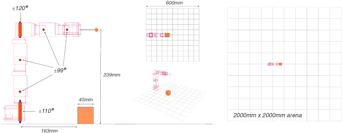
Figure 8. The robot is provided an object to interact with. Pictured here, the position zero of the robot, which corresponds to the start and target position for each movement.

We do not directly use the weights for parametrizing the motor space. Instead, we use the LWLR function approximator provided with the DMP library (Stulp, 2014), and define two linear functions per motor, with slopes a₀,a₁ and offsets b₀,b₁, respectively. The function approximator then computes the forcing term to approximate as much as possible these functions at time c₀ and c₁. Although directly manipulating the weights would be more natural, this method provides a rich diversity of trajectories, and, because DMPs were not a focus of our work, we did not inquire further about making the system perform better or making the representation more compact. Each motor has independent a₀,a₁,b₀,b₁ parameters, and the motors share σ₀, σ₁, while c₀,c₁ are fixed. With six motors, the motion trajectory of the robot is therefore parametrized by a vector of dimension 26. After solving and integrating the dynamical system, we obtain each motor angular position as a function of time.

To avoid the real robot removing (rather brutally) their own wires, the range of the first and fourth motor from the base are restricted to ±110° and ±120° (Figure 8). All other motors are physically restricted by their horns to ±99°. In simulation, the robot has the same angle constraints.

The ranges of the DMP parameters are set, so that 95% of the trajectories of a motor would fall in between the angles the motors were able to produce (using an empirical evaluation), and the rest are clipped to legal motor values.

Before executing the motion on the robot, we check for self-collisions, and collisions with the armature of the experiment. If present, the trajectory is truncated and stops just before the collision to avoid damage on the real robot. The same collision prevention methods are used in simulation, with the exception that the robot can collide freely with the ground.

5.1.2. Environment and Objects

The simulation is conducted using the robot simulator V-REP (Virtual Robot Experiment Platform), with the Open Dynamic Engine (ODE) as a physics engine backend. The environment features an object placed in a cubic arena. The robot arm can interact with the object and the ground.

We consider two sizes for the arena: 600 mm width and 2000 mm width. The larger arena approximates an unbounded environment, while interactions between the object and the walls are frequent in the smaller one. Unless indicated otherwise, we assume the 600-mm arena is used. Two different objects are used: a ball and a cube, of diameter and width both equal to 45 mm.

As a physics engine, ODE has many undesirable and chaotic behaviors that could be overexploited to produce diversity. For instance, movements where the robot pushes from the top of an object toward the ground yield large and significantly different object displacements over repeated executions.

As a preventive measure, we monitor the forces that are applied between the end effector of the robot and the rest of the environment. If at any point a reactive force exceeds 100 N, the simulation is discarded, and the sensory feedback that would be produced by an immobile robot is returned.

5.1.3. Sensory Primitive

At the end of the simulation, the trajectory of the object is processed by sensory primitives that compute the sensory feedback. We consider a simple sensory primitive that returns the displacement of the object projected on the ground at the end of the simulation. The displacement is returned as a vector of length 3: the displacement in x, in y, and a discrete dimension of saliency, which has value 0 if no collision happened, and 1 otherwise.

The saliency dimension helps separate observations that create collisions from one that do not. This is not crucial for the perturbation-based inverse model, but it makes the LWLR-based inverse model more robust.

5.1.4. Behavior of the Setup

The simulation environment does not yield repeatable results. Repeated executions of the same movement can generate significantly different effects, as shown in Figure 9A. Indeed, the random seed of the physics engine is not reset when the scene is reset.² As ODE uses the current state of the random generator to decide the order with which to resolve the constraints at each step, small variations are introduced that are amplified by the chaotic nature of the interaction with the objects.

FIGURE 9

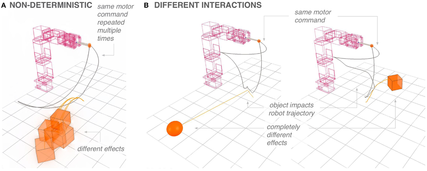
Figure 9. (A) The physics engine is chaotic. When the same motor command is reexecuted multiple times, the variations in object displacement are significant. (B) When reusing a motor command moving with the ball on the cube, the produced displacements can be quite different. Let us remark that the interaction with the object can largely impact the robot’s motion.

In Figure 9B, the same motor command is executed on the cube and ball task. The same motions do not generate necessarily similar effects on the objects. Moreover, the interaction with the object can significantly impact the trajectory of the end effector.

We ran experiments on the ball task (because the cube occupies more volume, the ball gives a lower estimate of the collision probability) to decide which number of motor babbling timesteps to use during the experiments. By tallying the number of collisions (not counting those that generate too much force) on a large number of random motor babbling steps (25,000), we estimate the probability to interact with the object during a movement at 2.87% for the cube and 1.81% for the ball. To ensure a high probability that every motor babbling phase had at least one collision, we set the bootstrapping phase to 200 steps (resulting in 99.17 and 97.40% probability of at least one collision for the cube and the ball, respectively).

5.2. Cube and Ball Experiments

In this section, we conduct several experiments with the ball and the cube task. All experiments are conducted in simulation. In all experiments, the coverage measure is computed with the radius, τ, set to 22.5 mm, which is the radius of the ball and the half-width of the cube.

5.2.1. Cubes and Balls

The first experiments look at how Reuse is effective when reusing the exploration of one object for another.

The source task is explored using the Explore algorithm with the perturbation-based inverse model (d = 0.05). The random motor babbling phase lasts 200 steps (K_boot = 200). The target task is explored with the Reuse algorithm, with the same inverse model, and 200 steps of bootstrapping as well. During the bootstrapping phase, each motor babbling step has a 50% probability to be replaced by a reuse steps (p_reuse = 0.5). In both cases, the exploration lasts 1000 steps in total.

Figure 10 depicts an execution of the Reuse algorithm. The cube is the source task, and the ball is the target task, compared with the ball task using the Explore algorithm. The impact of Reuse is visible during the bootstrapping phase: reusing motor commands from the cube exploration allows to move the ball in many directions in the first 200 steps. In the Explore case, only three interactions are made during that time.

FIGURE 10

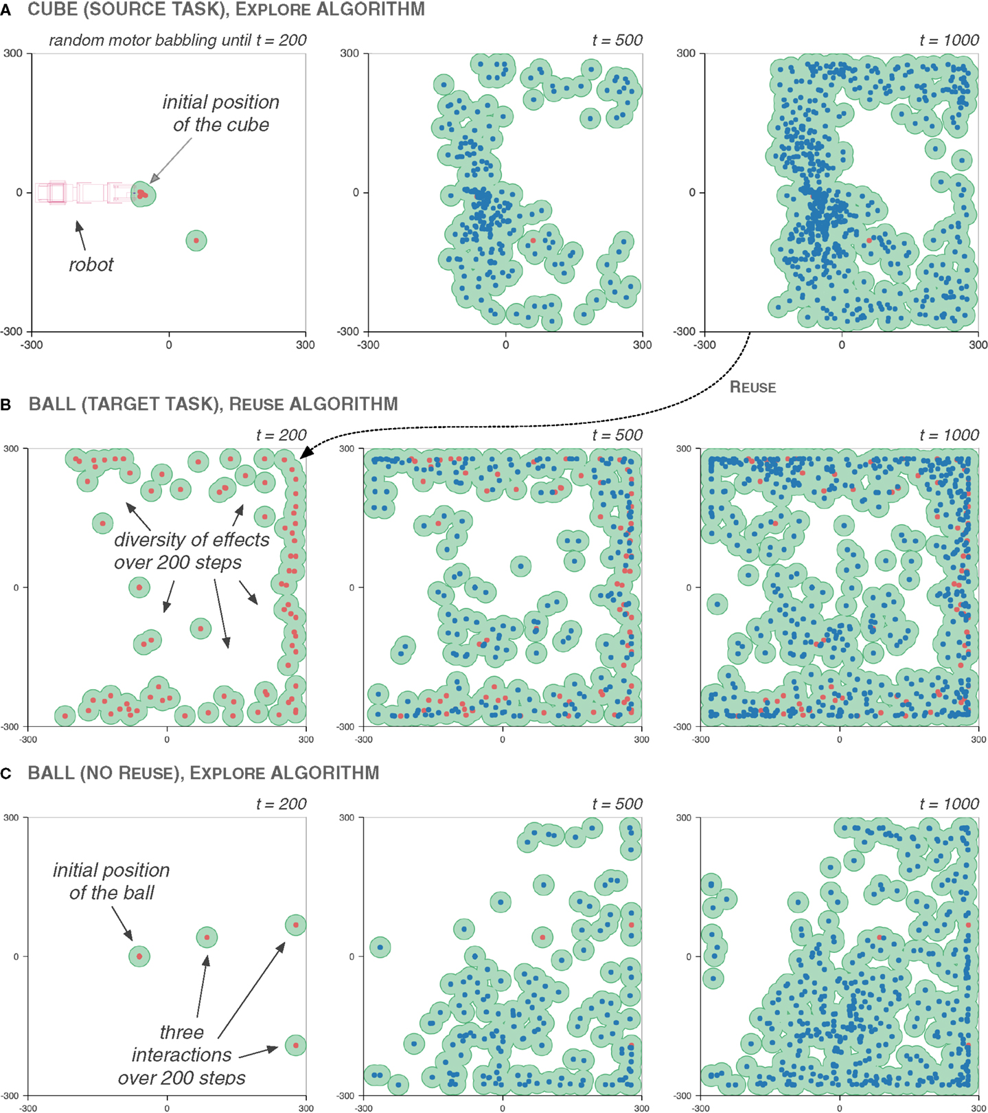
Figure 10. The coverage of the Reuse exploration benefits from a high diversity of effects during the bootstrapping phase. The graphs show the distribution of effects during the 200-step bootstrapping phase (in red), and during the subsequent goal-babbling phase (in blue), and the corresponding τ-coverage (in green, τ = 22.5 mm), across three explorations. The source task (A) is the cube task. It is used by the Reuse algorithm for the target task, the ball task (B). To compare the Reuse and the Explore algorithm, the exploration of the ball task under the Explore algorithm is presented in (C). Interestingly, we can see that during the exploration of the source task, the robot only learned to push the cube away. This has a notable influence on the exploration of the target task: the reused motor commands produce effects that also largely push the ball away. Even after the end of the goal babbling phase on the source task, the area surrounding the robot features fewer effects than the rest of the effect space. This illustrates the same sort of issue as the one discussed in Section 4. Still, in this case, the Explore algorithm does worse: with only three interactions after 200 steps, the exploration is biased toward the lower-right corner.

In Figure 11, the τ-coverage the four combinations of the cube and ball tasks is shown, for 25 repetitions of the experiment. The Reuse algorithm outperforms the Explore algorithm in all four cases, but the improvements are most important early in exploration. Moreover, when a task uses itself as a source, the impact of the Reuse algorithm is predictably better than when coming from the other object. This is mostly pronounced on the cube task: reusing the ball task is much less effective than when the cube task reuses itself.

FIGURE 11

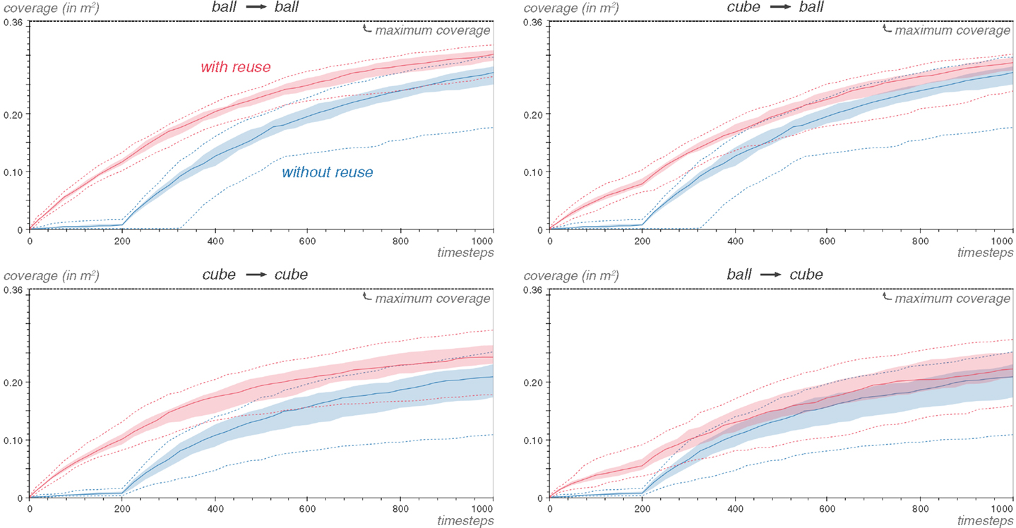
Figure 11. Whether reusing the cube on the ball task or the ball on the cube task, Reuse brings an important coverage boost early in exploration. The figure presents the median of the coverage for the Reuse and Explore cases in the four possible combinations of the cube and ball tasks. The shaded area is delimited by the 25th and 75th percentiles of 25 repetitions of each experiment, and the best and worst case is shown by dashed lines. The effect of Reuse is increased when reusing from the same task, and the ball task is able to exploit the cube task better than the reverse.

A likely explanation of this asymmetry lies in how differently the two objects respond to interaction: the ball will discriminate between most interactions, moving in slightly different directions, while many interactions with the cube will make it just tip over on one side. Therefore, the cube needs more pronounced motions of the robot to be displaced across the arena, whereas the ball only has to explore small variations of the same movements, which are less effective at generating diversity when reused on the cube.

5.2.2. Different Exploration Algorithms

So far, the source task and the target task have only differed in their exploration algorithm by a few random motor babbling steps replaced by Reuse steps. But the exploration of the source task in not constrained in any such way by the use of the Reuse algorithm.

We consider the case where the source task is explored by a pure random motor babbling strategy. At each of the 1000 steps of the exploration, a random motor command is chosen in the hyperrectangle M and executed. The parameters of the Reuse algorithm remain the same as before. Figure 12 shows the impact of such a change on the Reuse coverage.

FIGURE 12

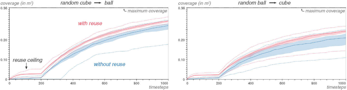
Figure 12. The Reuse method is able to exploit observations generated by random motor babbling. The source task in these graphs was explored using a pure random motor babbling strategy. Repeated 25 times.

The coverage is improved by reusing motor commands from a random motor babbling source, but less so than when using the Explore algorithm in the source task. The coverage hits a ceiling at around 50 steps into the bootstrapping phase, because the source task did not generate enough diversity to sustain the Reuse algorithm for 200 steps. This leads to the idea of shortening the bootstrapping phase: many times more interactions with the object have been discovered through Reuse after 50 steps than the Explore case will discover through random motor babbling in 200 steps. The goal babbling algorithm has enough observations to be effective.

Figure 13 demonstrates that this is a viable strategy. In the case of the ball task as source task, the coverage improvement in early exploration is actually much greater when the ball task is explored with random motor babbling than with the Explore algorithm (Figure 11).

FIGURE 13

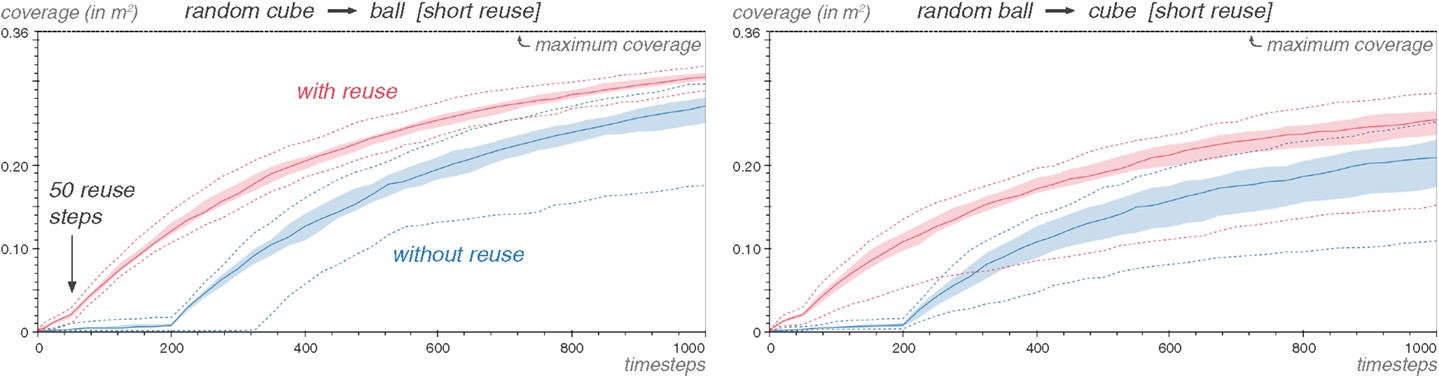
Figure 13. Reuse allows to shorten the bootstrapping phase. The K_boot parameter is equal to 50 steps in for the Reuse algorithm here. The source task is explored with random motor babbling. Repeated 25 times.

The effectiveness of the Reuse algorithm at exploiting a random motor babbling source also validates the selection process of the motor commands through the diversity of the effects they produced. Indeed, if Reuse was merely selecting random motor commands from the source task, the Reuse method would be equivalent to the random motor babbling strategy when reusing a random motor babbling source: randomly selecting samples from a random source is equivalent to directly sampling the random source. The improvement in coverage here can only be attributed, then, to the selection of motor commands through diversity.

5.2.3. Robustness to Dissimilarity

In the previous experiments, the cube and the ball share the same location relative to the robot. This is of course an important reason for the effectiveness of the Reuse algorithm. While there may be ways for the robot to adapt to such change and still be able to take advantage of Reuse – for instance, by having high-level motor primitives expressed in an object-centered reference frame – they are not the focus of this article.

However, an important consideration is to examine if the Reuse algorithm can decrease the performance of the exploration. The response is of course positive. One can construct a source and a target task so that wasting half of the random motor babbling phase on reusing motor commands guaranteed not to produce any interesting effects could negatively impact the exploration performance. Here, we show that the Reuse algorithm is reasonably robust to a change in the position of the object in the ball environment: some, but not much, of the performance is lost.

In the ball task, the ball is located just under the robot. The displaced task is in every way identical to the ball task, except that the ball has been moved on the right side of the robot. Most movements generating an interaction with a ball will not generate one with the other ball. Moreover, this ball is harder to hit with random movements, with an interaction probability of 0.99% (versus 1.81% before). This is important, because it means that if 100 movements are wasted on reexecuting motor commands that will not hit the ball, the probability of interacting with the ball goes from 86 to 63%.

This is reflected in the results, Figure 14. While the loss in coverage at the median is small, the difference is apparent at the 25th percentile in both cases. And the when the displaced task is the target task, the performance below the 25th percentile is much worse for Reuse than for Explore.

FIGURE 14

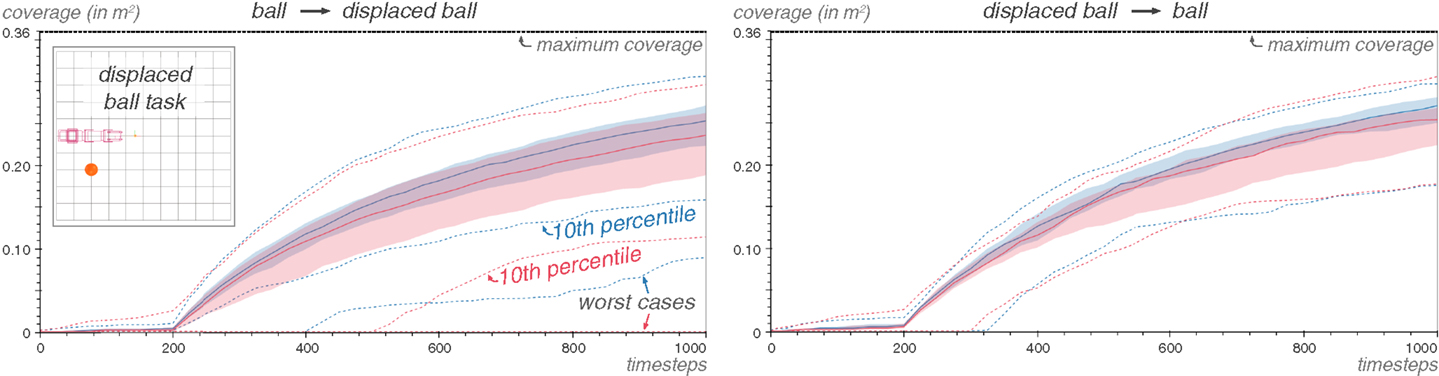
Figure 14. Reusing from a dissimilar ball task has no significant impact on performance. In the displaced task, the ball has been moved to the side of the robot, rendering most motor commands useful for interacting with the ball on one task useless in the other. Repeated 100 times.

While they are not explored here, there are several ways to prevent negative transfer. One is to decrease p_reuse, as it decreases the how the Reuse algorithm modifies the original Explore algorithm. When p_reuse is equal to zero, both algorithms are equivalent. Another possibility is to dynamically adjust p_reuse based on the relative performance of the two bootstrapping strategies: random motor babbling or reused motor commands. We have proposed an algorithmic framework to do precisely that in Benureau and Oudeyer (2015). Ultimately, the decision to use Reuse or not sometimes cannot be made inside the problem we defined: it must come from an external mechanism, which needs only to point out the existence of a relationship between tasks, without specifying it. We investigate an example where a caregiver could fill that role in the next section.

5.3. Scaffolding Diversity: The Pool Experiment

So far, the Reuse algorithm has brought quantitative improvements in coverage, most of the time in the early phase of the exploration. We now introduce an experiment that show that Reuse can radically affect how exploration happens: namely, that can allow to explore an environment that is difficult to explore directly.

We consider the pool task, where two balls are present in the arena, with one out of reach. The robot must strike the first ball and make it collide with the second ball to interact with it (Figure 15A). The second, out-of-reach ball is the only one that is perceived through the sensory primitive. Therefore, in response to the execution of a motor command, the exploration algorithm receives the displacement of the second ball only. The exploration algorithm is therefore unaware of any interaction with the first ball.

FIGURE 15

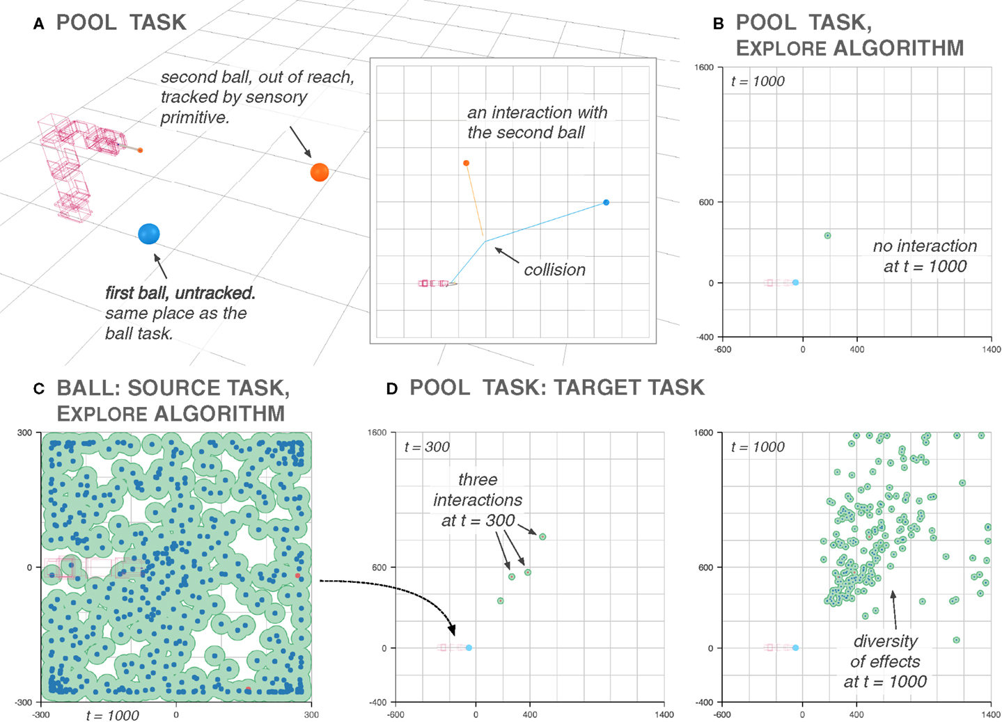
Figure 15. The Reuse algorithm helps discover difficult-to-find areas of the sensorimotor space. In the pool experiment, a ball (in orange) is placed out of reach and the only option to interact with it is to interact with another ball (in blue), which is not tracked by the sensory primitive (A). Exploring such an environment directly is difficult, because the odds of stumbling on an arm motion that leads to an interaction with the second ball are very low as demonstrated by an execution of the Explore algorithm (B). Using the ball task as a source (C), some of those interactions are easily discovered, and the goal babbling of the pool task can start creating diversity from them (D).

Exploring such a task with the Explore algorithm is inefficient. The probability of interacting with the first ball during the random motor babbling phase is low (1.81%). The probability of interacting with the first ball in such a way that it collides with the second ball is very low (0.04%). Even by setting K_boot to 300 steps as we do for this experiment, most of the time, no interaction is witnessed after the end of random motor babbling, and goal babbling cannot function without at least one observation of a collision (Figure 15B).

Discovering the possibilities offered by such an environment hinges on chance. Without guidance, no informative intervention can be carried out because the environment gives neither clues about the existence of such informative interventions nor any gradient to follow toward their location: this is the bootstrapping problem, similar to the one encountered in evolutionary robotics (Mouret and Doncieux, 2009). In a context where an agent must allocate its time efficiently between different learning situations, the pooltask will most probably be quickly abandoned with the conclusion that it does not offer anything to learn.

In such a context, the Reuse algorithm can provide a way to discover those interesting parts of the sensorimotor space in a reasonable amount of time. We use the ball task used in the previous sections as a source task for the pool task (Figure 15C). During the exploration of the ball task, the robot discovers how to move the ball in different directions. Through Reuse, the robot replays those movements on the pool task, moving the blue ball in different directions. Some of those movements make the blue ball strike the orange ball, and thus generate novel environmental feedback. The goal babbling algorithm is then able to explore different ways the second ball can be moved (Figure 15D).

By looking at the coverage of the Reuse versus Explore strategy over 100 repetitions of the experiment (Figure 16), we see that the 10th percentile of Reuse is better than the 90th percentile of the Explore strategy.

FIGURE 16

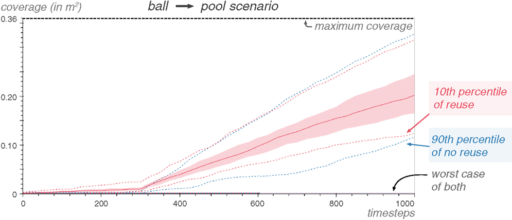
Figure 16. Most of the explorations with Explore never make the ball move in the pool environment. Using Reuse, however, the exploration of the second ball is consistently diverse, and 90% of the Reuse exploration generate strictly more coverage than the 90% of the explorations with the Explore algorithm.

This experiment showcases an important possibility offered by the Reuse algorithm: environment-driven exploration. By simply placing an agent inherently driven to explore to produce behavioral diversity, a caregiver can scaffold complex and directed behavior by manipulating the environment – here, by adding a ball – without giving any explicit goal or reward, and without the need to reprogram the robot.

The Reuse algorithm would work equally well if the source task already contained both balls, with the blue ball tracked instead of the orange one. In that scenario, the sensory primitive would encode the attention of the robot, and moving from the source to the target task only necessitates switching the attention from the blue ball to the orange one. This is another role that a caregiver could fulfill.

5.4. Hardware Setup

In this section, we present a hybrid simulation/hardware setup that was used to validate some results of the simulation. The setup features real robots, but the interaction with the object is done in a physics engine.

5.4.1. Hybrid Interactions

The robot (Figure 17) has a reflective marker at the tip, which allows to accurately capture its position at 120 Hz during its movement using an OptiTrack Trio camera system. A virtual marker then replays the trajectory in a simulation where a virtual object has been put. As the marker is the only part of the robot tracked by the camera, it is the only part of the robotic arm that is transposed in the simulation and therefore that can collide with the object.

FIGURE 17

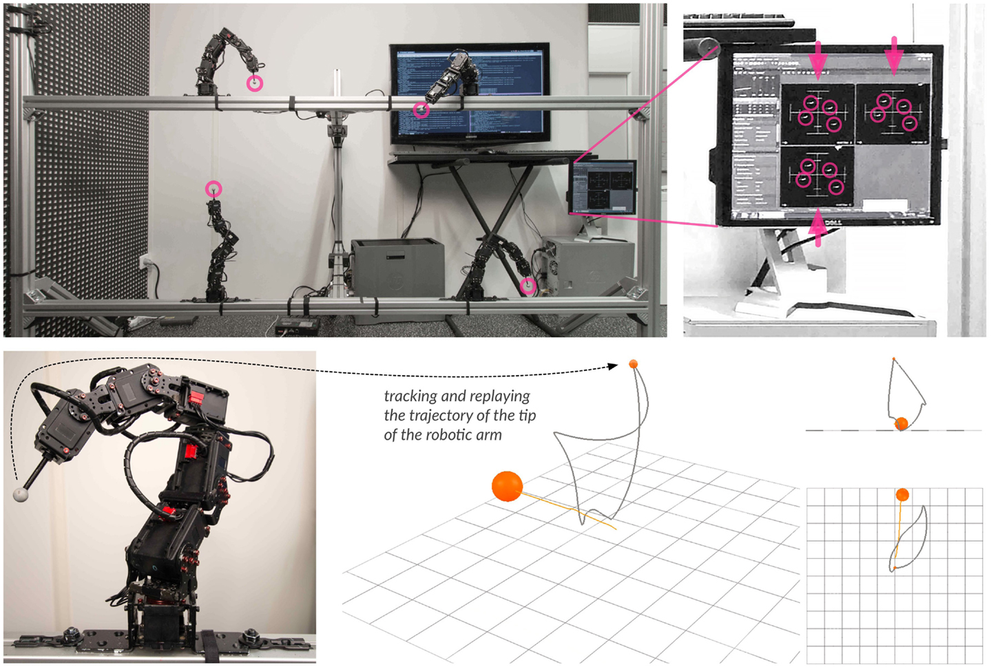
Figure 17. The hardware setup consists of four robots, separated so that they cannot interact with each other. The tracking system is positioned in front of the setup and has three cameras that capture the position of the four markers. The monitor on the right shows the detection mask of each camera. Most movements of the stems will keep the marker visible, but some will not. However, those movements will overwhelmingly be far away from the virtual objects as it involves the robots arching backward to block the view of the marker from the camera with their own body. Once the movement of the arm is finished, the trajectory of the marker is transposed and replayed into the simulation, where the interaction with the object happens.

Contrary to the fully simulated experiment, the simulated marker does not interact with the ground where the object rest and can therefore pass through it. Moreover, the immediate reaction force on the marker can exceed 100 N without the interaction being discarded.

We chose to use a real robot and a simulated environment for the simplicity and flexibility it affords. Tracking and resetting an object a few thousands of times requires some form of mechanism, or a bigger robot, which makes the experimental setup more complicated. Additionally, the robot never experiences physical collisions, which reduces the risk of damage when babbling, given the type of robot we had. And prototyping new environments, with new objects or layouts, is cheap and unconstrained.

At the same time, using a virtual environment for an interaction task removes some of the main source of interest of the setup: a realistic, difficult to simulate interaction with a real object with kinesthetic feedback. Still, the real robot and the cameras bring real sources of motor and sensory noise that are important to check against when studying the production of diversity.

5.4.2. Cube and Ball

We reproduce the cube and ball experiments on the real setup. This time, the inverse model used is the InverseLBFGSB-LWLR one, and the arena is 2000 mm by 2000 mm. This approximates an unbounded environment.

The results in Figure 18 show that Reuse is effective on the hardware setup. Because the arena is more than 10 times bigger than the 600 mm by 600 mm arena, the production of coverage does not level-off as fast. In particular, the pooling around the walls seen in Figure 10 is much less present. This explains why there is still a difference of coverage after 1000 steps between the Reuse and Explore algorithm. In situations where the time allowed to explore a task is finite and much lower than would be needed to discover all the possibilities of the environment, Reuse can therefore significantly increase the amount of knowledge discovered by a robot.

FIGURE 18

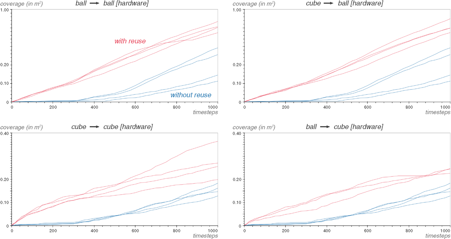
Figure 18. Reuse provides a head start to the exploration on the hardware setup. The coverage performance is shown for each repetition of the experiment. The arena is the 2000 mm width 1, and the inverse model used is InverseLBFGSB-LWLR.

5.5. Reality Gap Experiments

So far, we have shown that Reuse is effective in situations that involve switching the object (ball/cube experiment in Section 5.2), changes in the morphology of the robot (different link lengths in Section 4), or increased complexity (scaffolding experiments in Section 5.3). The purpose of using Reuse in these situations is to leverage past experiences to provide the locations of possible good mapping in the sensorimotor space.

In this section, we show that the Reuse method can be used to leverage experiences acquired in simulation on real robots, even when the simulation is not accurate.

5.5.1. The Reality Gap

Many experiments learning controllers for legged robots have reported remarkable performances for simulated robots. But far fewer have been able to transfer controllers learned in simulation onto real robots and preserve performance (Lipson et al., 2006; Palmer et al., 2009). In other words, the transfer from simulation to reality is not efficient: this is the reality gap problem (Jakobi et al., 1995; Jakobi, 1998). In robotics, the reality gap is overwhelmingly studied in the context of the optimization of controllers in simulation to be transferred on a real robot, in particular in the context of evolutionary robotics (Nolfi et al., 1994; Koos et al., 2013).

The most straightforward way to deal with the reality gap is to create the most accurate simulation possible. But this is fraught with problems, and leads to fragile and expensive simulations.

Some approaches improve the simulator during learning based on empirical observations (Bongard and Lipson, 2005; Bongard et al., 2006; Zagal et al., 2008; Koos et al., 2009). Other methods consider the simulator as fixed, and evaluate the mapping between the simulator and the reality. This allows to estimate the discrepancy between the two and to only perform simulated optimization in areas where the discrepancy is low (Koos et al., 2013).

5.5.2. Crude Simulations

With Reuse, we take a different approach. Instead of spending ever-increasing efforts to create or search for a realistic simulation, we go in the opposite direction; we search for a much simpler, much cruder simulation that still affords us an exploratory advantage through Reuse. Jakobi (1997) proposes a similar method where he identifies a minimal set of features responsible for the behavior of the robot, and simulates only those. But our approach is different still: our aim is not to transfer behaviors, but it is to transfer behavioral diversity.

To test this, we create a simplified kinematic simulation of the object interaction setup of Section 5.1. Instead of using a physics engine, we compute the trajectory of the end-effector by feeding the kinematic model with the joint trajectories produced by the motor primitives. Moreover, the object is approximated to its axis-aligned bounding box. If the trajectory of the end-effector enters the bounding box, the velocity of the end-effector is averaged from its last 10 positions, and the displacement of the object is computed as a vector of the same direction as the velocity of the end-effector, and with a norm proportional to the end-effector velocity. There is no floor to interact with, the displacement of the object is computed in three dimensions, and then projected on the x and y dimensions.

Under this model, there is no difference anymore between a ball and a cube. No contact is simulated except the one between the object and the end-effector, and the collisions are computed as if they were always directed toward the center of mass of the object.

The kinematic simulation is run for 1000 timesteps using the Explore exploration strategy (K_boot = 300, d = 0.05). The exploration is then transferred to the V-REP simulation of the ball task of Section 5.1. The exploration on the full simulation uses the Reuse algorithm and is parametrized with K_boot = 300, d = 0.05, and p_reuse = 50%. The results are available Figure 19.

FIGURE 19

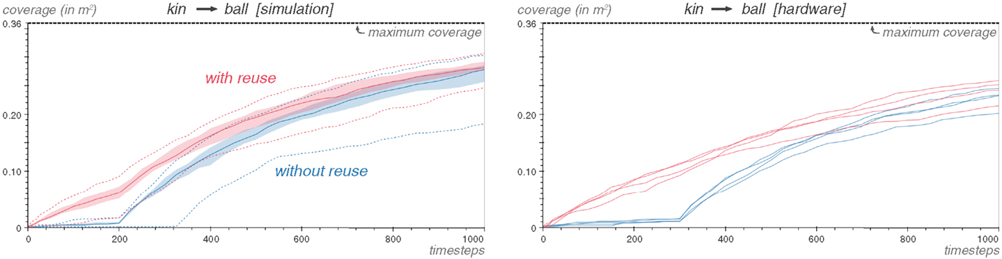
Figure 19. Even with a crude model, the Reuse transfer is effective. The simulation results show 25 repetitions with the median, the 25th and 75th percentile margins and the best and worst case in dashed lines. The experiment is repeated on the hardware four times. Each of the coverage curves for those repetitions is represented.

Even with a crude simulation devoid of most physical features, the Reuse strategy is able to take significant advantage of the generated data.

5.5.3. A Cruder Simulation

We simplify the previous simulation. Instead of computing the displacement of the object, the sensory response is only conditioned by the end-effector entering the bounding box. If that happens, a random value between 0 and 1 is returned. Else, a random value between −1 and 0 is returned. The sensory signal has only one dimension. This experiment also affords us with another example of Reuse being compatible with a change in sensory modalities.

Learning with such a poor sensory feedback is more difficult. The simulation has essentially become an indicator for a possible collision. Yet, Reuse still provides an improvement (Figure 20). As should be expected, the improvement is less than when the simulation is more informative.

FIGURE 20

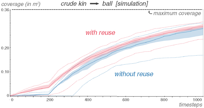
Figure 20. Even with a cruder model, the Reuse transfer is still effective. 25 repetitions.

A weakness of our reality gap experiments is that even a simple forward kinematic model usually displays good performance on a rigid body robotic arm. Although we removed many aspects of the physical simulation, we retained the essential part. The discrepancy then between a collision detected in simulation and one produced in reality is low. This easily explains the results obtained. And while we claimed not to assume that the simulation needs to be physically accurate, it actually is, but qualitatively.

The way the object displacement is computed in the first crude simulation can also be criticized. Although it seems that, by not taking into account any geometry of the object, or not considering the floor we have lost much information, the direction of the displacement is directly correlated to the direction of the end-effector when a collision happens. This sensory feedback is probably richer in information that the final position of the object in the physical simulation. It is also a signal that is easier to learn. The first crude simulation could be considered as a scaffolding that offers knowledge of a pivotal aspect of the interaction – the direction and velocity of the colliding tip of the arm just before the collision – that was hidden so far.

Of course, these criticisms can also be considered positively: yes, the crude models are qualitatively accurate with regards to the presence of a collision, and Reuse is able to take advantage of a merely qualitative, rather than numerical, accuracy.

In a self-sufficient perspective, the crude simulations could be considered as cognitive models. Their simplicity and relaxed qualitative nature makes their acquisition by a self-sufficient robot more reasonable than realistic simulations. Instead of reproducing reality, these cognitive simulations can do away with much of the realism while retaining power to direct and inform behavior. They pose as artifices of cognition that would allow robots, in some situations, to reason about the world without having to predict or simulate it accurately.

6. Related Works

Goal-directed exploration (Oudeyer and Kaplan, 2007; Baranes and Oudeyer, 2010; Jamone et al., 2011; Rolf et al., 2011; Baranes and Oudeyer, 2013), as well as related methods such as MAP-Elite (Cully et al., 2015), has been shown to be effective at creating behavioral diversity in large sensorimotor spaces. However, these methods only consider a single task. The Reuse algorithm proposes to transfer the behavioral diversity from one task to another. It, therefore, works particularly well when combined with these strategies as we have demonstrated in this paper.

The Reuse method is an instance of a transfer algorithm. Machine learning algorithms improve their prediction or control capabilities from data. Transfer learning algorithms (Thrun and Pratt, 1998; Taylor and Stone, 2009; Pan and Yang, 2010) aim at improving their prediction or control capabilities on a problem either from another problem’s existing data or more directly from the other problem’s learned prediction or control capabilities. In other words, transfer learning expands the scope of the data that can be used on a specific problem.

Therefore, transfer learning is typically used when not enough data is available to obtain the desired performance. Creating a zebra classifier can be difficult if only a few labeled pictures are available. While a horse classifier does not address the exact same problem, enough commonalities exist between the two for useful information to be extracted from the horse classifier and used in the zebra one.

Transfer learning algorithms have been historically developed for tasks where unlabeled data is plentiful, but labeling is expensive; robots face a similar labeling problem. Every motor action a robot undertakes is costly in time and energy. Therefore, while the motor action possibilities are numerous, only a small fraction of them can be executed to observe the environmental response they produce – i.e., labeled – during the time allotted to learn a problem. Transfer learning in robots allows to make use of the observations acquired outside of the current problem.

Many different methods have been developed on how, what, and when to transfer data from one task to another, and the interested reader can consult Thrun and Pratt (1998), Taylor and Stone (2009), Pan and Yang (2010), and Lazaric (2012) for reviews.

In evolutionary robotics, Velez and Clune (2014) shows that controllers evolved in a first maze through Novelty Search (Lehman and Stanley, 2011), i.e., with the incentive to behave differently from the rest of the population, provide a head start on the exploration of a second maze. In comparison with Reuse, the transferred controllers are valued not because they solve different tasks, or explore the maze differently: they are issued from independent runs, and all solve the same task, going to the same predefined goal. Rather, they are valued because they can adapt faster to the new task than random controllers, having acquired exploration abilities in the first maze. In the Intelligent Trial and Error algorithm (IT&E) (Cully et al., 2015), a performance map is generated by MAP-Elite on a task and then reused to find a fast adaptation to a different task. However, the performance mapping is used to guide the search, which is focused on a specific objective.

In reinforcement learning, an interesting method comes from Sherstov and Stone (2005) that creates a set of tasks from a source task, and prune the action space from any action that is not optimal in at least one task of the set. The diversity of the set of tasks creates a filter that is used to reduce diversity in the set of actions.

In the context of Markov-Decision Processes (MDP), policy reuse (Fernández and Veloso, 2006) builds a library of policy. Each policy corresponds to a specific reward function over the MDP. Each time a new reward function needs to be learned, the most similar policy in the policy library is reused probabilistically with a ε-greedy strategy. The policy reuse algorithm focuses on learning how to solve a single reward function at a time, over discrete or discretized domains. Like IT&E, it uses the reward function to decide which policy to reuse.

We first exposed the Reuse method in Benureau and Oudeyer (2013). The Transfer was driven by intrinsic motivation then. It was changed to a diversity-driven method in Benureau et al. (2014) but the empirical results presented then were limited to the content of Sections 5.2.3 and 5.4.2. This paper provides a comprehensive empirical study and investigates many different situations: changes in morphology, sensory modalities, and the exploitation of a random motor babbling source. The effectiveness of Reuse is explained by showing how the diversity of two different tasks can be highly correlated, and we investigates the details of a situation where Reuse, at his worst, is less efficient than the worst-case without it. The paper also makes two major new contributions: the application of Reuse to scaffolding behavior (Section 5.3) and exploiting simulation results on real robots (Section 5.5).

7. Discussion

7.1. Synthesis

Sensorimotor spaces present difficulties that preclude an isolated approach. They typically feature a large motor space that cannot be explored exhaustively. Rather, often, only a few small regions of it are actually interesting to explore for any practical purpose. The difficulty, of course, lies in discovering those regions. However smart an exploration algorithm is, when the environment does not provide clues or gradient toward those regions, finding them relies on chance.

The Reuse method proposes a way to discover these small regions of interesting behavior by relying on past experience. In an autonomous context where neither experts nor peers are present, and in a developmental context where robots are supposed to accumulate experience about the world over large periods of time, relying on past experience seems trivially self-evident. It can prove, however, challenging. A strength of the Reuse method is that it makes easy to use past experiences that would otherwise be considered incompatible with the current situation. We have provided examples of the Reuse method adapting to changes in objects (cube and ball, Section 5.2), in morphology (length of arm links in Section 4), in task dissimilarity (change in the ball position, Section 5.2.3), in sensory modalities (coordinate systems in Section 4 and crude simulation in Section 5.5.3), in complexity (pool experiment in Section 5.3), and in execution context (from simulation to reality in Section 5.5).

Yet, the Reuse method remains, at its heart, remarkably simple: create a collection of actions having generated a diversity of effects in a previous task, and optimistically reexecute them in the new one. As a consequence, the method is algorithmically cheap. The only constraint is that actions from the source task must be reexecutable in the target task.

While the Reuse method makes many past experiences suddenly compatible with the current situation, it does not mean that they are relevant or beneficial. The planar arms experiments (Section 4) provided us with evidence that complex interactions between the tasks, the inverse model and the Reuse method may worsen the exploration in some cases rather than help it. And much of the success of the Reuse method lies in the similarity between the tasks. When the two tasks are too dissimilar, the Reuse method needs to degrade gracefully, and this is what the experiment with the displaced task demonstrated (Section 5.2.3).

The Reuse method does not merely improve or accelerate the exploration of sensorimotor spaces. As the pool experiment illustrates (Section 5.3), it can scaffold the exploration of difficult environments. It allows a caregiver to guide the exploration of an autonomous agent, leading it to acquire specific and sophisticated behaviors, without specifying an explicit goal or reward, by either directing the attention or manipulating the environment.

The Reuse method also seems naturally suited to propose solutions to a difficult problem: exploiting simulation results on real robots. The Reuse method does this by side-stepping the difficulty of preserving performance. Instead, it focuses on preserving behavioral diversity, providing good starting points in the sensorimotor space of the real robot (Section 5.5). Moreover, our experiment with crude simulations suggests that cheap cognitive models can efficiently serve an efficient source of behavioral diversity, informing the exploration in the real world and in full-featured simulations.

7.2. Limitations and Perspectives

The works presented here suffers many limitations. The Reuse algorithm is only analyzed with regards to the behavioral diversity it creates through the τ-coverage metrics and not on the quality of either the predictive or control models that can be derived from the observations it generates. This should be investigated in future works, especially in context where robots must apply their skills and knowledge to reach specific goals.

This leads us to the issue of chaotic environments, evoked in Section 3. In the full simulation of the interaction task (Section 5.1), we monitored the reactive forces to mitigate the chaotic behavior of the physics engine. More generally, chaotic areas of the sensorimotor spaces generate behavioral diversity that is difficult to exploit for practical purposes. To make Reuse more robust to these aspects, the chaotic and stochastic characteristics of the reused motor command should be explicitly evaluated.

Another blind spot of the Reuse algorithm is motor command diversity. When the effect diversity of the source task is low, motor commands producing similar effects are reused. In such a case, choosing motor commands according to how different they are from one another would increase the diversity of the set of transferred commands. This would make Reuse robust to scenarios where, for instance, all motor commands produce the same effect in the source task.

Another venue of improvement would be to make Reuse active, i.e., aware of its own effect of the exploration. By having a feedback on its performance, the algorithm could dynamically decide to modify the value of p_reuse or of the length of the bootstrapping phase (Section 5.2.2). This could also lead to Reuse identifying which parts of the source task observations produce the most diversity on the target tasks, and to preferentially to Reuse motor commands from those areas: this could have been exploited in the pool experiment in particular (Section 5.3).

In this paper, we have only considered one source task. But Reuse should be expanded to multiple tasks scenarios, since autonomous developmental robots are not expected to have only one explored task in their past experience.

The experimental setups presented in this paper do not yet allow to generalize to many robotic contexts. The algorithm should be tested in more diverse environments, with different sensory primitives, and in particular fully autonomous, real-world ones.

Author Contributions

Ideas and design: FB (75%) and P-YO (25%), experiments: FB (100%), code: FB (100%), writing: FB (75%), and P-YO (25%).

Conflict of Interest Statement

The authors declare that the research was conducted in the absence of any commercial or financial relationships that could be construed as a potential conflict of interest.

Acknowledgments

Thanks to Paul Fudal, whose engineering expertise made the experiments on object interaction possible. Thanks to Thomas Cederborg for his helpful comments during the redaction of the manuscript.

Funding

This work was partially funded by the ANR MACSi and the ERC Starting Grant EXPLORERS 240 007. Computing hours for running simulations were graciously provided by the MCIA Avakas cluster.

Supplementary Material

The source code and data for reproducing the experiments and producing all graphs, as well as the provenance data of the experiments and instructions to recreate the computational environments is published (Benureau and Oudeyer, 2016) and is made available at: https://dx.doi.org/10.6084/m9.figshare.2816284

Footnotes

1. ^The source code and data for producing all graphs is published (Benureau and Oudeyer, 2016) and is made available at https://dx.doi.org/10.6084/m9.figshare.2816284
2. ^This is an implementation detail of V-REP, and there was no way to change it the version we used.

References

Atkeson, C. G., Moore, A. W., and Schaal, S. (1997a). “Locally weighted learning,” in Lazy Learning, ed. D. W. Aha (Dordrecht: Springer), 11–73.

Google Scholar

Atkeson, C. G., Moore, A. W., and Schaal, S. (1997b). “Locally weighted learning for control,” in Lazy Learning, ed. D. W. Aha (Dordrecht: Springer), 75–113.

Google Scholar

Baldassarre, G., and Mirolli, M. (eds) (2013). Intrinsically Motivated Learning in Natural and Artificial Systems. Berlin, Heidelberg: Springer Science + Business Media.

Google Scholar

Baranes, A., and Oudeyer, P.-Y. (2013). Active learning of inverse models with intrinsically motivated goal exploration in robots. Rob. Auton. Syst. 61, 49–73. doi: 10.1016/j.robot.2012.05.008

CrossRef Full Text | Google Scholar

Baranes, A., and Oudeyer, P.-Y. (2010). “Intrinsically motivated goal exploration for active motor learning in robots: a case study,” in IEEE/RSJ International Conference on Intelligent Robots and Systems (Taipei: IEEE), 1766–1773.

Google Scholar

Benureau, F., Fudal, P., and Oudeyer, P.-Y. (2014). “Reusing motor commands to learn object interaction,” in Proceedings of ICDL-Epirob 2014, IEEE, Genoa.

Google Scholar

Benureau, F., and Oudeyer, P.-Y. (2013). “Autonomous reuse of motor exploration trajectories,” in Proceedings of ICDL-Epirob 2013, 1–8.

Google Scholar

Benureau, F., and Oudeyer, P.-Y. (2015). “Diversity-driven selection of exploration strategies in multi-armed bandits,” in ICDL-EPIROB 2015, Providence, RI.

Google Scholar

Benureau, F., and Oudeyer, P.-Y. (2016). Code and data for “Behavioral Diversity Generation in Autonomous Exploration Through Reuse of Past Experience”. doi:10.6084/m9.figshare.2816284.v1

CrossRef Full Text | Google Scholar

Bonawitz, E. B., van Schijndel, T. J. P., Friel, D., and Schulz, L. (2012). Children balance theories and evidence in exploration, explanation, and learning. Cogn. Psychol. 64, 215–234. doi:10.1016/j.cogpsych.2011.12.002

PubMed Abstract | CrossRef Full Text | Google Scholar

Bongard, J., and Lipson, H. (2005). Nonlinear system identification using coevolution of models and tests. IEEE Trans. Evol. Comput. 9, 361–384. doi:10.1109/tevc.2005.850293

CrossRef Full Text | Google Scholar

Bongard, J., Zykov, V., and Lipson, H. (2006). Resilient machines through continuous self-modeling. Science 314, 1118–1121. doi:10.1126/science.1133687

PubMed Abstract | CrossRef Full Text | Google Scholar

Byrd, R. H., Lu, P., Nocedal, J., and Zhu, C. (1995). A limited memory algorithm for bound constrained optimization. SIAM J. Sci. Comput. 16, 1190–1208. doi:10.1137/0916069

CrossRef Full Text | Google Scholar

Cazals, F., Kanhere, H., and Loriot, S. (2011). Computing the volume of a union of balls. ACM Trans. Math. Softw. 38, 1–20. doi:10.1145/2049662.2049665

CrossRef Full Text | Google Scholar

Cleveland, W. S., and Devlin, S. J. (1988). Locally weighted regression: an approach to regression analysis by local fitting. J. Am. Stat. Assoc. 83, 596–610. doi:10.1080/01621459.1988.10478639

CrossRef Full Text | Google Scholar

Cook, C., Goodman, N. D., and Schulz, L. E. (2011). Where science starts: spontaneous experiments in preschoolers’ exploratory play. Cognition 120, 341–349. doi:10.1016/j.cognition.2011.03.003

CrossRef Full Text | Google Scholar

Cully, A., Clune, J., Tarapore, D., and Mouret, J.-B. (2015). Robots that can adapt like animals. Nature 521, 503–507. doi:10.1038/nature14422

PubMed Abstract | CrossRef Full Text | Google Scholar

Fernández, F., and Veloso, M. (2006). “Probabilistic policy reuse in a reinforcement learning agent,” in Proceedings of AAMAS 2006, AAMAS ’06, ACM, 720–727.

Google Scholar

Gopnik, A. (1997). Words, Thoughts, and Theories. Cambridge, MA: MIT Press.

Google Scholar

Gopnik, A. (2012). Scientific thinking in young children: theoretical advances, empirical research, and policy implications. Science 337, 1623–1627. doi:10.1126/science.1223416

PubMed Abstract | CrossRef Full Text | Google Scholar

Gopnik, A., Sobel, D. M., Schulz, L. E., and Glymour, C. (2001). Causal learning mechanisms in very young children: two-, three-, and four-year-olds infer causal relations from patterns of variation and covariation. Dev. Psychol. 37, 620–629. doi:10.1037/0012-1649.37.5.620

PubMed Abstract | CrossRef Full Text | Google Scholar

Gweon, H., and Schulz, L. (2008). “Stretching to learn: ambiguous evidence and variability in preschooler’s exploratory play,” in Proceedings of the 30th Annual Meeting of the Cognitive Science Society (Austin, TX: Cognitive Science Society), 1552–1556.

Google Scholar

Hoffmann, M., and Pfeifer, R. (2012). The Implications of Embodiment for Behavior and Cognition: Animal and Robotic Case Studies. ArXiv e-prints.

Google Scholar

Ijspeert, A. J., Nakanishi, J., Hoffmann, H., Pastor, P., and Schaal, S. (2013). Dynamical movement primitives: learning attractor models for motor behaviors. Neural Comput. 25, 328–373. doi:10.1162/neco_a_00393

PubMed Abstract | CrossRef Full Text | Google Scholar

Ijspeert, A. J., Nakanishi, J., and Schaal, S. (2002). “Movement imitation with nonlinear dynamical systems in humanoid robots,” in Proceedings of the 2002 IEEE International Conference on Robotics and Automation (ICRA), (Washington, DC: IEEE), 1398–1403.

Google Scholar

Jakobi, N. (1997). Evolutionary robotics and the radical envelope-of-noise hypothesis. Adapt. Behav. 6, 325–368. doi:10.1177/105971239700600205

CrossRef Full Text | Google Scholar

Jakobi, N. (1998). “Running across the reality gap: octopod locomotion evolved in a minimal simulation,” in Evolutionary Robotics: First European Workshop, EvoRobot98 Paris, France, April 16–17, 1998 Proceedings, eds P. Husbands and J.-A. Meyer (Springer Science + Business Media), 39–58.

Google Scholar

Jakobi, N., Husbands, P., and Harvey, I. (1995). “Noise and the reality gap: the use of simulation in evolutionary robotics,” in Advances in Artificial Life: Third European Conference on Artificial Life Granada, Spain, June 4–6, 1995 Proceedings, eds F. Morán, A. Moreno, J. J. Merelo, and P. Chacón (Berlin, Heidelberg: Springer Science + Business Media), 704–720.

Google Scholar

Jamone, L., Natale, L., Hashimoto, K., Sandini, G., and Takanishi, A. (2011). “Learning task space control through goal directed exploration,” in IEEE International Conference on Robotics and Biomimetics (ROBIO) (Karon Beach: IEEE), 702–708.

Google Scholar

Koos, S., Mouret, J.-B., and Doncieux, S. (2009). “Automatic system identification based on coevolution of models and tests,” in Proceedings of the 2009 IEEE Congress on Evolutionary Computation, (CEC) (Trondheim), 560–567.

Google Scholar

Koos, S., Mouret, J.-B., and Doncieux, S. (2013). The transferability approach: crossing the reality gap in evolutionary robotics. IEEE Trans. Evol. Comput. 17, 122–145. doi:10.1109/tevc.2012.2185849

CrossRef Full Text | Google Scholar

Kulvicius, T., Ning, K., Tamosiunaite, M., and Worgötter, F. (2012). Joining movement sequences: modified dynamic movement primitives for robotics applications exemplified on handwriting. IEEE Trans. Robot. 28, 145–157. doi:10.1109/TRO.2011.2163863

CrossRef Full Text | Google Scholar

Lazaric, A. (2012). “Transfer in reinforcement learning: a framework and a survey,” in Reinforcement Learning: State-of-the-Art, eds M. Wiering, and M. Otterlo (Berlin, Heidelberg: Springer Science + Business Media), 143–173.

Google Scholar

Lehman, J., and Stanley, K. O. (2011). Abandoning objectives: evolution through the search for novelty alone. Evol. Comput. 19, 189–223. doi:10.1162/evco_a_00025

PubMed Abstract | CrossRef Full Text | Google Scholar

Lipson, H., Bongard, J., Zykov, V., and Malone, E. (2006). “Evolutionary robotics for legged machines: from simulation to physical reality,” in Proceedings of the 9th International Conference on Intelligent Autonomous Systems, 11–18.

Google Scholar

Loeb, G. E. (2012). Optimal isn’t good enough. Biol. Cybern. 106, 757–765. doi:10.1007/s00422-012-0514-6

CrossRef Full Text | Google Scholar

Lorenz, K. (1996). “Innate bases of learning,” in Learning as Self-Organization, eds K. H. Pribram and J. S. King (Mahwah, NJ: L. Erlbaum Associates), 1–56.

Google Scholar

Morales, J. L., and Nocedal, J. (2011). Remark on “algorithm 778: L-BFGS-B: Fortran subroutines for large-scale bound constrained optimization.” ACM Trans. Math. Softw. 38, 1–4. doi:10.1145/2049662.2049669

CrossRef Full Text | Google Scholar

Moulin-Frier, C., Nguyen, S. M., and Oudeyer, P.-Y. (2014). Self-organization of early vocal development in infants and machines: the role of intrinsic motivation. Front. Psychol. 4:1006. doi:10.3389/fpsyg.2013.01006

PubMed Abstract | CrossRef Full Text | Google Scholar

Moulin-Frier, C., and Oudeyer, P.-Y. (2013). “Exploration strategies in developmental robotics: a unified probabilistic framework,” in IEEE Third Joint International Conference on Development and Learning and Epigenetic Robotics (ICDL). Osaka: IEEE.

Google Scholar

Mouret, J.-B., and Doncieux, S. (2009). “Overcoming the bootstrap problem in evolutionary robotics using behavioral diversity,” in IEEE Congress on Evolutionary Computation (Trondheim: IEEE), 1161–1168.

Google Scholar

Munzer, T., Stulp, F., and Sigaud, O. (2014). “Non-linear regression algorithms for motor skill acquisition: a comparison,” in Proceedings JFPDA (Liège), 1–16.

Google Scholar

Nolfi, S., Floreano, D., Miglino, O., and Mondada, F. (1994). “How to evolve autonomous robots: different approaches in evolutionary robotics,” in Artificial life IV: Proceedings of the 4th International Workshop on Artificial Life (MA: MIT Press), 190–197.

Google Scholar

Oudeyer, P.-Y., and Kaplan, F. (2007). What is intrinsic motivation? a typology of computational approaches. Front. Neurorobot. 1:6. doi:10.3389/neuro.12.006.2007

PubMed Abstract | CrossRef Full Text | Google Scholar

Palmer, M., Miller, D., and Blackwell, T. (2009). “An evolved neural controller for bipedal walking: Transitioning from simulator to hardware,” in Proceedings of IROS 2009 Workshop on Exploring New Horizons in Evolutionary Design of Robots.

Google Scholar

Pan, S. J., and Yang, Q. (2010). A survey on transfer learning. IEEE Trans. Knowl. Data Eng. 22, 1345–1359. doi:10.1109/TKDE.2009.191

CrossRef Full Text | Google Scholar

Penrose, R., and Todd, J. A. (1955). A generalized inverse for matrices. Math. Proc. Cambridge Philos. Soc. 51, 406. doi:10.1017/s0305004100030401

CrossRef Full Text | Google Scholar

Rolf, M., Steil, J., and Gienger, M. (2011). “Online goal babbling for rapid bootstrapping of inverse models in high dimensions,” in Proceedings of ICDL 2011, Vol. 2, (Frankfurt am Main), 1–8.

Google Scholar

Schulz, L. E., and Bonawitz, E. B. (2007). Serious fun: preschoolers engage in more exploratory play when evidence is confounded. Dev. Psychol. 43, 1045–1050. doi:10.1037/0012-1649.43.4.1045

PubMed Abstract | CrossRef Full Text | Google Scholar

Schulz, L. E., Gopnik, A., and Glymour, C. (2007). Preschool children learn about causal structure from conditional interventions. Dev. Sci. 10, 322–332. doi:10.1111/j.1467-7687.2007.00587.x

PubMed Abstract | CrossRef Full Text | Google Scholar

Sherstov, A. A., and Stone, P. (2005). “Improving action selection in mdp’s via knowledge transfer,” in Proceedings of the 20th National Conference on Artificial Intelligence, AAAI’05, Vol. 2, Pittsburgh: AAAI Press.

Google Scholar

Stulp, F. (2014). DmpBbo – A C++ Library for Black-Box Optimization of Dynamical Movement Primitives.

Google Scholar

Taylor, M. E., and Stone, P. (2009). Transfer learning for reinforcement learning domains: a survey. J. Mach. Learn. Res. 10, 1633–1685.

Google Scholar

Thrun, S., and Pratt, L. (eds) (1998). Learning to Learn. (Boston, MA: Springer Science + Business Media), 3–17. doi:10.1007/978-1-4615-5529-2

CrossRef Full Text | Google Scholar

Till, M. S., and Ullmann, G. M. (2009). McVol – a program for calculating protein volumes and identifying cavities by a Monte Carlo algorithm. J. Mol. Model. 16, 419–429. doi:10.1007/s00894-009-0541-y

CrossRef Full Text | Google Scholar

Velez, R., and Clune, J. (2014). “Novelty search creates robots with general skills for exploration,” in Proceedings of the 2014 Conference on Genetic and Evolutionary Computation – GECCO ’14 (Vancouver, BC: ACM), 737–744.

Google Scholar

Zagal, J. C., Ruiz-del Solar, J., and Palacios, A. G. (2008). “Fitness based identification of a robot structure,” in Artificial Life XI: Proceedings of the Eleventh International Conference on the Simulation and Synthesis of Living Systems, eds S. Bullock, J. Noble, R. Watson, and M. A. Bedau (Cambridge, MA: MIT Press), 733–740.

Google Scholar

Zhu, C., Byrd, R. H., Lu, P., and Nocedal, J. (1997). Algorithm 778: L-BFGS-B: fortran subroutines for large-scale bound-constrained optimization. ACM Trans. Math. Softw. 23, 550–560. doi:10.1145/279232.279236

CrossRef Full Text | Google Scholar