Social Skill Acquisition Model through Face-to-Face Interaction: Local Contingency for Open-Ended Development

1. Introduction

Joint attention is one of the most basic cognitive functions in human communication. It is simply defined as looking where someone else is looking (Butterworth and Jarrett, 1991), and extensive research has been conducted by those investigating the developmental process of following the gaze of others (Butterworth and Jarrett, 1991; Corkum and Moore, 1995; Moore et al., 1997), including a report that a human infant shows this capability before birth (Scaife and Bruner, 1975). These results have garnered research interest in cognitive science and developmental psychology owing to its important role in the acquisition of social capabilities, such as language communication and mind reading (Moore and Dunham, 2014). Recently, a number of research efforts in the field of robotics have focused on the issue of joint attention in human–robot interaction (Kaplan and Hafner, 2006) as it also appears to be a necessary building block in this type of interaction. The development of robotics technologies and a consequent possible future for human society with interactive robots adds to the importance of studies on joint attention, which has implications for creating communicative robots (Imai et al., 2003; Kanda et al., 2004).

Understanding the developmental process of the human infant by producing an infant model based on the utilization of synthetic approaches (Asada et al., 2009) has also garnered increasing research interest. The role of joint attention-related behavior is also being explored in this research area in an effort to understand the mystery surrounding the development of a human being (Nagai et al., 2003; Triesch et al., 2006). These synthetic studies focused on the significant role of joint attention behavior in the acquisition of social skills through the interaction of a human infant with its caregiver. They considered the causality between gaze behavior of the infant and the caregiver, and proposed that a robotic model of an infant could acquire social behavior, such as gaze following, by acquiring sensorimotor mapping from the face pattern of the caregiver to its own motor command by estimating the causality among them. In these works, the programmer had to specify the set of variables on which the robot should focus to learn the sensorimotor mapping. However, to acquire various types of social behavior, the programmer needed to redefine the set of variables for each of the behavioral types. Therefore, a mechanism to automatically find the appropriate sets of variables seems to be necessary to apply the learning robot in different interactive scenes in different environments.

Oudeyer et al. addressed intrinsic motivation for the learning robot, which enables open-ended development (Oudeyer et al., 2007). They showed how an internal reward system that equates a lower prediction error with a larger reward enables the learning robot to automatically acquire various types of behavior in an incremental manner. However, they did not consider the sequential properties of human behavior in the interaction in depth, which seems to be essential for continuing the interaction. For example, when a robot becomes more social by learning to respond to a human in an appropriate way, the human will try to continue the interaction with it by, for example, talking to it or touching it in response to its reaction. Therefore, by learning actions that result in contingent sequences, a robot would be able to continue such interactions with the human.

Mugan and Kuipers extended the reinforcement learning method to incrementally acquire dynamic Bayesian networks for modeling predictable events in a continuous environment (Mugan and Kuipers, 2012). Because a longer sequence of events gradually becomes predictable by sequentially combining the models found, it can be used to plan the hierarchy of the actions to accomplish the given tasks, ranging from simple tasks, such as hitting an object, to complex ones, such as grabbing the object. However, it is difficult to apply this method to learning social skills through social interaction, because the tasks that have to be accomplished in the interaction are not always (or even rarely) explicitly given. Furthermore, the pure predictability of the events is considered to evaluate the causality of the events, which is implemented by dynamic Bayesian networks. Therefore, causalities that are independent of the state of others are included in the found causalities. In other words, there is no mechanism to detect and avoid these causalities, which leads the robot to be incapable of choosing a suitable action for interacting with the human through social interaction.

In recent studies, Sumioka et al. (2008) derived a contingency evaluation measure focusing on the effect of a robot’s own action only in relation to specific conditions, including those reflecting the state of others. An informational theoretical measure based on transfer entropy (Schreiber, 2000) was utilized for the evaluation, and applied to the model of an infant robot interacting with a human caregiver model in a computer simulation. The result shows that evaluating contingency among variables leads the robot to find a combination of the variables that should be focused on to acquire a sensorimotor mapping, which enables the robot to behave in a social way, such as performing gaze following and social referencing. Regarding the gradual changes of the response of the caregiver model with the emergence of the infant-robot’s communicative abilities, which were designed based on those reported for the interaction of a human caregiver with its infant (Bruner et al., 1982; Adamson and Bakeman, 1984), the robot obtained a meaningful response from the caregiver model when it used an acquired social skill. For example, the caregiver model had a strict rule such as looking at the robot when the robot successfully performed the acquired gaze following skill. Therefore, the robot could find further contingency between “using the gaze following skill” and “consequent face direction of the caregiver” (which is looking at the robot due to the strict rule). This contingency was expressed as a chain of contingencies, which consists of a sequence of two consequences: (1) finding the object (by following the gaze of the caregiver) and (2) finding the caregiver’s frontal face (by looking at the caregiver after gaze following).

In Sumioka et al. (2010), they focused on the importance of the sequence of contingent sub-actions in several social behaviors of human infant, where lots of them such as social referencing behavior consist of these sequences. Therefore, they extended the mechanism to find the chain of contingencies by evaluating contingency among the skill that was used, the action that was taken, and the consequent observation of the robot. However, in their method, the acquisition of complex skills, i.e., skills consisting of a contingency chain, is too time consuming; in addition, they did not sufficiently check whether complex skills with longer sequences could be acquired. Accordingly, only the acquisition of the simple skills is reported in the implementation of this system in a real-world robot (Sumioka et al., 2013). Moreover, the performance of this mechanism is not compared with the results obtained by others, such as Oudeyer et al. (2007) and Mugan and Kuipers (2012), in which simple concepts, such as the pure predictability of the events for the evaluation of the causalities, are used.

In this paper, we propose a mechanism to overcome these two significant problems, namely poor skill acquisition and the large number of time-consuming steps. Our proposed mechanism is based on two main ideas. First, we introduce a new informational measure, named transfer information, which evaluates contingency among specific values of variables. Previously (Sumioka et al., 2008, 2010, 2013), the expectation of contingency among whole values of the variables was utilized to evaluate contingencies. Therefore, gathering a sufficient number of samples for all values of the variables was highly time consuming. Instead, in the proposed method, it is sufficient to gather samples of specific values of the variables for the evaluation. In this way, fast contingency evaluation is realized in the proposed method. Second, we utilize transfer information to produce a measure that evaluates the synergistic contribution of values in contingencies. It enables the robot to distinguish the contingencies, which consist of the synergistic effect of taking a specific action in a specific state to the environment, from those composed of a single effect. This approach leads the robot to acquire more complex skills, i.e., skills with a longer contingency chain and interaction sequences, compared with work by other researchers.

In the results section of this paper, we compare the performance of our proposed mechanism with those of others using computer simulation: work that utilizes simple concepts, such as predictability for the skill acquisition process of the robot, such as Oudeyer et al. (2007) and Mugan and Kuipers (2012); and work that uses more complex concepts, such as finding saliency of contingencies among variables to prevent the acquisition of a huge number of behavioral rules, as well as those unrelated to the state of the interacting person, such as Sumioka et al. (2008, 2010), and (Sumioka et al., 2013). In this paper, the former is implemented using transfer information to evaluate events at the value level (locally), whereas the latter utilizes transfer entropy that evaluates events at the variable level (globally). We refer to these methods as “local pure predictability method” (l.p. method) and “global contingency method” (g.c. method), respectively. For comparison, we consider the interactive environment used in Sumioka et al. (2010), but the measure used in the skill acquisition process of the robot differs for each method.

The remainder of this paper is organized as follows: first, we describe the assumed interactive scene of the robot with its caregiver in our experiment. Then, we explain the system schema of the proposed mechanism and its components. After that, we analyze the results of the two experiments, i.e., the computer simulation performed to validate our system. In the first simulation, we compare the performance of the proposed method with the other mechanisms in a simplistic interactive world model. In this comparison, accuracy and speed of skill acquisition as well as robustness against uncertainty is examined. In the second simulation, we examine whether our system remains feasible when the robot has additional sensing and action modalities and the caregiver behaves accordingly based on more complex rules. It shows the capacity of the proposed mechanism for application in a more complex environment, such as in real-world interaction between robots and humans.

2. Mechanism

We assume a face-to-face interaction between a human caregiver and an (infant) robot (Figure 1). In each time step, the robot observes its environment and sends action commands to its joints. The robot obtains the observation as sensory variable S, and taken action as action variable A. In addition, the robot retains the resultant observation after taking the action as resultant variable R. These variables consist of some elements, S_i (i = 1, 2, …, N^s; N^s denotes the number of types of sensory data), A_j ( j = 1, 2, …, N^a; N^a denotes the number of different kinds of actions), and R_k (k = 1, 2, …, N^k; N^k denotes the number of types of resultant sensory data), respectively.

FIGURE 1

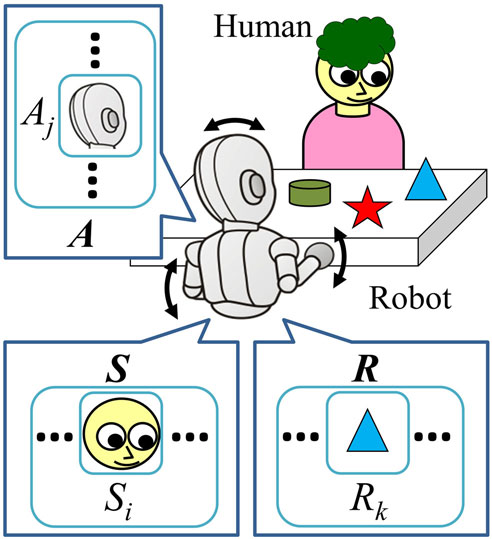
Figure 1. Interactive environment: a human caregiver interacting with a robot across a table.

Figure 2 shows the structure of the proposed mechanism. The system consists of two main components: a contingency detecting unit (CDU) and an action producing unit (APU). After the observation of the current state at time t, i.e., updating the variables S^t and R^t, the APU produces an action for each joint of the robot (A^t) based on the current state. The robot observes the consequent result of taking action A^t, and saves it as R^t+1. The CDU evaluates the contingency based on the variables S^t, R^t, A^t, and R^t+1. If the CDU detects contingency, it adds a new contingency reproducer (CR) to the APU, which enables the robot to reproduce the found contingency by taking suitable action when it is observing a specific state. The action is mentioned as A* in Figure 2. Therefore, at the beginning, there is no CR in the APU; the APU produces action based on the output of another component, named the reaction producer (RP). The RP is designed to enable the robot to take pre-programed reactive action to a specific observation. The RP outputs suggested action A* in each time step. To produce many reactions, the system can have several RPs, from RP₁ to RP_NR. A component named Action Selector, finally, selects the outputting action to each joint of the robot, among the suggested actions A* from the RP and the CR (if any). Therefore, at the beginning of the interaction of the robot with the caregiver, the APU outputs the action based on the A* produced by RPs. Continuing the interaction leads the CDU to find contingency and add CRs to the APU. After that, the Action Selector chooses the outputting action A^t from the A* of the CRs and the RPs. The robot continues the interaction and continues acquiring additional CRs if there are further contingencies during the interaction. In this section, we explain each of the components in detail.

FIGURE 2

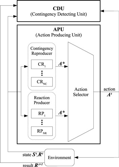
Figure 2. System schema.

Note that the global structure of the g.c. and l.p. method that we implemented for the comparison are same with the proposed mechanism, which have/will be described in this section/following subsections. In the last part of the following subsections, we will mention about them if there is any difference among the proposed method and the g.c./l.p. methods. For the detail of the g.c. method, see Sumioka et al. (2010).

2.1. Contingency Detection Unit

The CDU has two roles: detecting contingent experiences and generating new CRs based on them. It tries to find the contingencies using a histogram of experiences obtained through the interaction. The CDU is equipped with an informational measure to evaluate the contingency of the experiences. Once an experience is judged to be contingent, a CR is added to the APU to enable the robot to “reproduce” the contingency, i.e., take a suitable action in a specific state to be able to repeat the experience. We define the quaternion $\mathit{\text{e}}=\left(r_k^{t+1},s_i^t,a_j^t,r_k^t\right)$, where $r_k^{t+1},r_k^t\in R_k$, $a_j^t\in A_j$, and $s_i^t\in S_i$ as an experience. It indicates that in state $s_i^t$ taking the action $a_j^t$ made the transition of $r_k^t$ to $r_k^{t+1}$.

Using this definition, the system tries to learn the knowledge “when, what to do, for which transition.” It is expressed as acquiring social skills in our study.

2.1.1. Evaluating Contingency

Assume that X and Y denote two discrete-time stochastic processes that could be approximated by a stationary Markov process. When X takes the value x^t at time t, the evolution of the process is described by the transition probability p(x^t+1|x^t). Using transfer entropy (Schreiber, 2000), the dependency of the process X on the process Y can be quantified as:

$T_{Y\to X}={\displaystyle \sum _{x^{t+1},x^t,y^t}}p\left(x^{t+1},x^t,y^t\right)\log \frac{p\left(x^{t+1}|x^t,y^t\right)}{p\left(x^{t+1}|x^t\right)}.$ (1)

In other words, transfer entropy evaluates the effect of process Y on the transition of process X. We introduce “transfer information” that estimates the effect of a specific value of process Y, i.e., y^t, on the specific transition of process X, i.e., x^t to x^t+1 as follows:

$I_{y\to x}=\log \frac{p\left(x^{t+1}|x^t,y^t\right)}{p\left(x^{t+1}|x^t\right)}.$ (2)

If the value of the transfer information is high, it shows that the specific transition of x^t to x^t+1 has high dependency on the specific value y^t. We refer to this dependency as local contingency, or simply “contingency.” It is named local, because it does not evaluate the (averaged) dependency among all values of the processes (such as transfer entropy); instead, it performs the evaluation among the specific values of these processes.

Applying this to our environment, we can evaluate the effect of the specific values of the sensory variable S_i, i.e., $s_i^t$, and the action variable A_j, i.e., $a_j^t$, on the specific transition of the resultant variable R_k, i.e., $r_k^t$ to $r_k^{t+1}$, by the following equations, respectively:

$I_{s_i\to r_k}=\log \frac{p\left(r_k^{t+1}|s_i^t,r_k^t\right)}{p\left(r_k^{t+1}|r_k^t\right)}$ (3)

$I_{a_j\to r_k}=\log \frac{p\left(r_k^{t+1}|a_j^t,r_k^t\right)}{p\left(r_k^{t+1}|r_k^t\right)}.$ (4)

In other words, they evaluate the contingency of a specific transition on a specific state and action, respectively. Moreover, the joint effect of the specific values of the sensory variable and the action variable can be evaluated with the following equation:

$I_{\left(s_i,a_j\right)\to r_k}=\log \frac{p\left(r_k^{t+1}|s_i^t,a_j^t,r_k^t\right)}{p\left(r_k^{t+1}|r_k^t\right)}.$ (5)

In other words, it evaluates the contingency of a specific transition on a specific action in a specific state. Considering an experience $\mathit{\text{e}}=\left(r_k^{t+1},s_i^t,a_j^t,r_k^t\right)$, we can evaluate the local contingency of the experience on the state $s_i^t$, on the action $a_j^t$, or on the action $a_j^t$ in the state $s_i^t$, using equations (3) to (5), respectively:

$L_s\left(e\right)=I_{s_i\to r_k}$ (6)

$L_a\left(e\right)=I_{a_j\to r_k}$ (7)

$L_{\mathit{sa}}\left(e\right)=I_{\left(s_i,a_j\right)\to r_k}.$ (8)

We term them “single” contingencies (of experience e) on $s_i^t$, on $a_j^t$, and “joint” contingencies on $\left(s_i^t,a_j^t\right)$, respectively. However, evaluation of the joint contingency may reflect the contingency only on either $s_i^t$ or $a_j^t$, but not on both of them. To evaluate the synergistic contribution of both of the values $\left(s_i^t,a_j^t\right)$ on the joint contingency, we need to eliminate the contribution of single values, $s_i^t$ and $a_j^t$. The following equations eliminate the single contribution of values $s_i^t$ and $a_j^t$, respectively:

${}^{S}E\left(e\right)=\log \frac{p\left(r_k^{t+1}|s_i^t,a_j^t,r_k^t\right)}{p\left(r_k^{t+1}|s_i^t,r_k^t\right)}=L_{\mathit{sa}}\left(e\right)-L_s\left(e\right)$ (9)

${}^{A}E\left(e\right)=\log \frac{p\left(r_k^{t+1}|s_i^t,a_j^t,r_k^t\right)}{p\left(r_k^{t+1}|a_j^t,r_k^t\right)}=L_{\mathit{sa}}\left(e\right)-L_a\left(e\right).$ (10)

In the first equation, the transition probability $p\left(r_k^{t+1}|s_i^t,a_j^t,r_k^t\right)$ in the numerator is compared with $p\left(r_k^{t+1}|s_i^t,r_k^t\right)$ in the denominator. This compares the contribution of $\left(s_i^t,a_j^t\right)$ on the transition of $r_k^t$ to $r_k^{t+1}$, with the single contribution of $s_i^t$. In other words, it compares the dependency of the transition of $r_k^t$ on $\left(s_i^t,a_j^t\right)$ with the dependency on $s_i^t$. Therefore, ^SE(e) shows the difference of contributions on joint contingency between those of $\left(s_i^t,a_j^t\right)$ and $s_i^t$. In other words, it eliminates the single contribution of $s_i^t$ on the joint contingency. According to equations (3), (6), and (5), (8), ^SE(e) could be written as the subtraction of L_s(e) from L_sa(e). For the same reason, ^AE(e) eliminates the single contribution of $a_j^t$ on the joint contingency. To eliminate both of the single contributions and to achieve the synergistic contribution of the values on the joint contingency, the following measure could be used:

$E(e)-\min {\{}^{s}E(e),{}^{A}E(e)\}.$ (11)

Using this measure, the robot would be able to distinguish the experiences which are dependent on both of s_i and a_j, i.e., reflecting the knowledge “when ($s_i^t$), what to do ($a_j^t$), for which transition ($r_k^t$ to $r_k^{t+1}$).” The robot uses this measure to evaluate experiences in the proposed mechanism.

Note that the measure used in the g.c. method for the evaluation is designed based on transfer entropy, which evaluates contingency among the variables S_i, A_j, and R_k (Sumioka et al., 2010):

$\begin{array}{llll}\hfill C_{i,k}^j& =T_{\left(S_i,A_j\right)\to R_k}-\left(T_{S_i\to R_k}+T_{A_j\to R_k}\right)& \hfill & \\ \hfill & ={\displaystyle \sum _{\begin{array}{l}{r}_k^{t+1},r_k^t\in R_k\\ s_i^t\in S_i,a_j^t\in A_j\end{array}}}p\left(r_k^{t+1},s_i^t,a_j^t,r_k^t\right)\log \frac{p\left(r_k^{t+1}|s_i^t,a_j^t,r_k^t\right)p\left(r_k^{t+1}|r_k^t\right)}{p\left(r_k^{t+1}|s_i^t,r_k^t\right)p\left(r_k^{t+1}|a_j^t,r_k^t\right)}.\end{array}$ (12)

Furthermore, the l.p. method uses L_sa(e) for the evaluation, which reflects the (pure) predictability of the experience e, without elimination of the single contributions of the values on the joint contingency, such as those done in the equation (9) or (10).

2.1.2. Adding New CR to the APU

In each time step of the interaction, the robot calculates E(e) for all experiences utilizing their histograms. If the robot experiences specific e more than θ times and E(e) is higher than the acquisition threshold C_T, the robot accepts it as a contingent experience and adds a new CR to the APU based on it. Using the CR, the robot tries to reproduce the contingent experience in the next steps of the interaction. Each CR is mentioned as π_e based on the experience e that the CR is generated.

When a CR π_e is added to the APU, the CDU adds a new binary sensory variable S^π to the set of the sensory variable S. The new variable indicates whether π_e has been used in the previous time step; it takes the value “1” if it has, and “0” otherwise. The CDU then continues evaluating the E(e) of the experiences, including the new variable S^π. As a result, the CDU can evaluate a chain of contingencies stemming from the use of the found contingency, i.e., the contingencies relying on more than one time step related to the generated CR. Note that the CDU does not count experiences that do not contain S^π, when the robot has used an acquired π_e. We expect this trick to lead the CDU to focus on the effect of using acquired π_e on the environment, and consequently to enable the robot to evaluate contingency chains in shorter time steps.

Note that g.c. and l.p. method uses $C_{i,k}^j$ [equation (12)] and L_sa(e) [equation (7)] instead of E(e) which described above, respectively.

2.2. Action Producing Unit

The APU obtains the current state of the robot, and outputs an action to each joint of the robot (see Figure 2). The unit consists of three components: (1) contingency reproducer (CR), which suggests an action that leads to reproduce found contingency, (2) reaction producer (RP), which suggests an action designed to produce a specific reaction to a specific state, and (3) Action Selector, which chooses the outputting actions to each joint of the robot from those suggested.

2.2.1. Contingency Reproducer

The CR obtains the current state of the robot, and outputs a suggested action to reproduce the found contingency. It is generated by the CDU and added to the APU as mentioned in Section 2.1. Assume that a CR π_e is created with $e=\left(r_k^{t+1},s_i^t,a_j^t,r_k^t\right)$ where $r_k^{t+1},r_k^t\in R_k$, $a_j^t\in A_j$, and $s_i^t\in S_i$. Each CR is a sensorimotor mapping, which maps the robot’s current state $\left(s_i^t,r_k^t\right)$ to a suggested action a*; therefore, it is expressed as follows:

$a^{\ast }=f\left(s_i^t,r_k^t\right),$ (13)

where $f\left(s_i^t,r_k^t\right)$ indicates the sensorimotor mapping of π_e, which outputs $a_j^t$ as a*. The CR sends the a* to the Actions Selector together with its predictability Z. We use ^AE(e) as the measure reflecting the predictability of CR [see equation (10)], because it considers the cases in which the robot has/has not taken the action a* in the state $\left(s_i^t,r_k^t\right)$, and compares their transition probability to the desired observation [i.e., comparing $p\left(r_k^{t+1}|s_i^t,a^{\ast },r_k^t\right)$ with $p\left(r_k^{t+1}|s_i^t,r_k^t\right)$]. If the ^AE(e) is high, it means that taking action a* in the state $\left(s_i^t,r_k^t\right)$ increases the probability of achieving desired observation r^t+1, or in other words, the predictability of π_e is high.

To enable comparability with previous works (Sumioka et al., 2008, 2010, 2013), we mention the CR using another notation $\mathrm{\Pi }\left(R_k^{t+1}=r_k^{t+1}|S_i^t=s_i^t,A_j^t=a_j^t,R_k^t=r_k^t\right)$, which means that in state $\left(r_k^t,s_i^t\right)$ the CR suggests the action $a_j^t$ to reproduce the found contingency and expects the resultant observation $r_k^{t+1}$. We denote the expected resultant observation of CR with r*. In addition, to indicate the variables and the values separately, we may use the notifications Π(R_k|S_i, A_j) and $\mathrm{\pi }\left(r_k^{t+1}|s_i^t,a_j^t,r_k^t\right)$ for the CR, respectively. Both of them are labels we use to indicate the contingency reproducer, the former shows the policy on the specific variables, whereas the latter shows it on the specific values.

Note that in l.p. method, L_sa(e) [equation (7)] is used as the predictability Z, because it reflects the (pure) predictability of the experience e. For the g.c. method, refer to Sumioka et al. (2010).

2.2.2. Reaction Producer (RP)

The RP obtains the current state of the robot and outputs a suggested action to produce a pre-programed reaction to a specific state. It sends the suggested action to the Action Selector as well as its predictability Z. An RP sends a constant value α as the predictability. To simplify the quantitative analysis of the research result, in this work we assumed one RP for the system, which outputs a random action for any inputting state.

2.2.3. Action Selector

The Action Selector selects one action among candidates from the RP and the CR for each joint of the robot, regarding their predictability Z. Assume that the number of candidate actions generated by the RPs and CRs for a specific joint j are $N_j^R$ and $N_j^C$, respectively. We use a soft-max action selection method to calculate the probability of selecting the action suggested from component i for joint j:

$P_i^j=\frac{\exp \left(Z_i∕\mathrm{\tau }\right)}{{\sum }_{k\in N_j^R+N_j^C}\exp \left(Z_k∕\mathrm{\tau }\right)},$ (14)

where Z_i is the predictability of component i, and τ is a temperature constant. Note that if Z_i is reduced to less than the omission threshold C_O, the action selector does not consider that component as an input. With this mechanism, the system can refrain from using the CRs that have been incorrectly acquired. The calculated contingency of a CR usually decreases after the acquisition due to the probabilistic feature of the environment, such as unpredictability. We set C_O = C_T − ε to enable the system to tolerate such a feature, where C_T is the acquisition threshold (see section 2.1.2) and ε is a constant value. Furthermore, to avoid the acquisition of contingency chains that consist of a chain of the same actions for the same results, such as executing the same behavior for several time steps in a static environment and having consistent observation, the Action Selector does not use those CRs that do not change the observation, i.e., r* = r^t.

3. Computer Simulation

In this section, we discuss the two experiments we conducted to evaluate our proposed mechanism using computer simulation. In the first experiment, we compared the performance of our system with the g.c. and l.p. methods (see section 1) in terms of precision and recall, i.e., F-measure, learning speed, length of the acquired sequence of skills, and noise tolerance, to determine whether our system is more suitable for real-world implementation. In the second experiment, we implemented our system in a more complex environment to verify its ability to find (more complex) rules produced by a more complex caregiver model, and acquire (more complex) social skills related to these rules.

The basic assumptions used in the experiments were the same as those adopted by Sumioka et al. (2010). The environment used in the experiments is illustrated in Figure 1. The environment comprises a robot and a human caregiver sitting across a table, and an object on the table. There are n possible positions on the table for the object, and the caregiver moves it to a random spot every m time steps. In the experiments, we set (n, m) = (3, 10). We set the other simulation parameters as (θ, α, ε) = (8, 0, 0.1) based on our experiences (see sections 2.1.2, 2.2.2, and 2.2.3 for the parameters, respectively).

3.1. The First Experiment

We utilized a simplistic environment for the first experiment because comparison of the performance of the systems would be difficult in a complex environment. We considered a small number of sensory/action/resultant variables for the robot, and a corresponding small number of behavioral patterns for the caregiver model. Consequently, we were able to determine the combinations of variables and values that should be evaluated as a contingent experience. In other words, we were able to compile a list of CRs the robot should acquire in the experiment before performing the computer simulation. This made it possible to evaluate and compare the performance of the systems using F-measure, i.e., the harmonic mean of precision and recall of the skill acquisition algorithm. To enable a fair comparison, we first determined the best threshold parameter C_T for each system. This parameter is denoted as $C_T^{\ast }$ and produces the best performance, i.e., the highest F-measure, of the system. Then, we analyzed the learning speed, length of the acquired sequence of CRs, and noise tolerance to demonstrate the level by which our proposed method improved on that achieved previously by others. In this experiment, we set the constant parameter as τ = 0.3 (see section 2.2.3).

3.1.1. Experimental Setup

The same variables as those used by Sumioka et al. (2010) were utilized in this experiment (see Table 1). The sensory variable, S, consisted of two elements, the visual pattern of the caregiver’s face (S₁) and existence of the object (S₂). The action variable, A, consisted of two elements, gaze direction (A₁) and hand gesture (A₂). Lastly, the resultant sensory variable, R, consisted of three elements, the frontal face of the caregiver (R₁), the profile of the caregiver (R₂), and existence of object (R₃). S₁ could be one of five values: f₁, f₂, and f₃, which indicate the visual pattern of the caregiver’s face when the caregiver looks at either of the positions on the table; f_r, which indicates when the caregiver looks at the robot; and f_ϕ, which indicates that the robot was not able to detect the caregiver’s face. S₂ could have one of two values: o, which indicates that the robot has detected an object, and o_ϕ, which indicates the opposite situation. A₁ could be one of four values: g₁, g₂, and g₃, which indicate whether the robot is looking at the corresponding spot on the table; and g_c, which indicates that it is looking at the caregiver. A₂ could also have one of four values: h₁ − h₄, which indicates that the robot has made the corresponding hand gestures. If the robot was able to sense the frontal face of the caregiver, profile of the caregiver, and existence of the object, the value of the resultant variables R₁, R₂, and R₃ became one; otherwise, it was set to zero.

TABLE 1

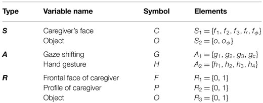
Table 1. Variable setup for the experiment.

3.1.2. Caregiver Model

We adopted simpler rules for the behavior of the caregiver by simplifying the rules used by Sumioka et al. (2010) to facilitate easier quantitative analysis of the performance of the system. In each time step, the caregiver either looked at the object or the robot in a random manner (OR-behavior). The only exception was when the robot followed the caregiver’s gaze direction. In such a case, the caregiver would look back at the robot with probability P_LB (LB-behavior). In this experiment, we set P_LB = 1.0. This setting enabled us to guess which experience would be acquired as the CR, and consequently, which contingency chains would be detected.

3.1.3. Expected Contingencies

The simplistic implementation of the caregiver model in a simplistic environment allowed us to infer the contingencies that would be found and acquired as CRs by the robot. By analyzing all combinations of the variables and their values in terms of whether any dependencies exist among their current and future values, we can find the combinations that should be treated as contingent experiences. Namely, through these analyses, the proposed method is expected to find the following combinations as CRs:

• First, the gaze following skill, GF, is expected to be acquired. Since the caregiver always looks at either the object or the robot, the robot should be able to find an object if it follows the gaze of the caregiver when the caregiver is looking at the object. The CR is Π_GF(R₃ = 1|A₁ = g_j, R₃ = 0, S₁ = f_i) where i = j and i = {1, 2, 3}. This contingency is related to the transition from time t to t + 1; hence, it expresses transition in one time step. Therefore, we define the “level” of this contingency as one. Let $S_{\text{GF}}^{\mathrm{\Pi }}$ be a sensory variable that represents whether the robot used Π_GF in the previous time step.

• Second, we expect the gaze returning skill, GR, to be acquired. This is a complex skill in which the robot returns its gaze to the caregiver after using the acquired skill of gaze following, i.e., GF, which leads it to perceive the face of the caregiver from the front. Since the caregiver looks at the robot with high probability (P_LB = 1) after the GF behavior, ${\mathrm{\Pi }}_{\text{GR}}\left(R_1=1|A_1=g_c,R_1=0,S_{\text{GF}}^{\mathrm{\Pi }}=1\right)$ should have a high value for E(e) and be found by the CDU. This contingency expresses a transition in two time steps, from t − 1 to t, and then from t to t + 1; therefore, the level of this contingency is two. Let $S_{\text{GR}}^{\mathrm{\Pi }}$ be a sensory variable that signifies whether the robot used Π_GR in the previous time step.

• The next expected skill, which is named “object looking after gaze returning” (OL), is a complex skill with a level of three. Acquisition of this skill enables the robot to look back at the previous place where the object had been found after using GR and lead it to find the same object again. The CR is ${\mathrm{\Pi }}_{\text{OL}}\left(R_3=1|A_1=g_i,R_3=0,S_{\text{GR}}^{\mathrm{\Pi }}=1\right)$, where i = {1, 2, 3}. The g_i is the same as that used in the two preceding steps, i.e., used in GF. This contingency is at level three because it is based on three transitions: from t − 2 to t − 1 by GF, from t − 1 to t by GR, and from t to t + 1 by itself. Let $S_{\text{OL}}^{\mathrm{\Pi }}$ be a sensory variable that signifies whether the robot used Π_OL in the previous time step.

• Finally, a complex skill at level four was also expected. After using OL, keeping the gaze direction at the current place should result in reconfirmation of the current object. This skill is denoted as OL2, with ${\mathrm{\Pi }}_{\text{OL}2}\left(R_3=1|A_1=g_i,R_3=1,S_{\text{OL}}^{\mathrm{\Pi }}=1\right)$, where i = {1, 2, 3}. Its contingency belongs to four transition steps: from t − 3 to t − 2 by GF, from t − 2 to t − 1 by GR, from t − 1 to t by OL, and from t to t + 1 by itself, therefore its level is four.

These contingencies are referred to in the evaluation of the system performance, in the next section, as those which should be acquired by the robot. As mentioned above, a consistent and simple behavior rule of the caregiver model in combination with a simplistic environment ensures that the robot is not disturbed in its attempts to detect and acquire the skills. However, there is another contingency that is not counted in the evaluation of the system performance in the next section, because it could be acquired or not. It is named “Object Permanency” (OP) and the CR is mentioned as ${\mathrm{\Pi }}_{\text{OP}}\left(R_3=1|A_1=g_i,R_3=1,S_{\text{GF}}^{\mathrm{\Pi }}=1\right)$, where i = {1, 2, 3}. The g_i is the same as that used in a step before, i.e., used in GF. It means that after using GF, keeping the gaze in the same direction leads to reconfirmation of the same object. However, the acquisition of GR disturbs the acquisition of OP, because in the state $S_i=S_{\text{GF}}^{\mathrm{\pi }}$, GR outputs $A_1=a_{\mathit{GR}}^{\ast }=g_c$, since OP needs the experience of A₁ = g₁/g₂/g₃ in that state, to be experienced and acquired by the robot. Conversely, the acquisition of OP does not disturb the acquisition of GR, because the Action Selector will not choose the output of acquired OP while $r_{\mathit{OP}}^{\ast }=r_{\mathit{OP}}^t$ (see section 2.2.3 for the selection prevention algorithm). Therefore, OP is not counted in the evaluation of the next section.

3.1.4. Results and Discussion

In this section, we compare the performance of three different methods: the proposed, g.c., and l.p. methods. The performance is expressed as the accuracy of each method in terms of the acquisition of CRs, and defined as their F-measure:

$F=2\cdot \frac{\text{precision}\cdot \text{recall}}{\text{precision}+\text{recall}}.$ (15)

For the calculation of precision and recall, the CRs listed in 3 are counted as the relevant elements. An acquired CR is regarded as true positive if it is listed in 3, and false positive otherwise.

However, the number of true positives and false positives are strongly affected by the value of acquisition threshold C_T. A large value of C_T leads to the acquisition of only those experiences with very high contingency as CR (or even not to acquire any CR), whereas setting C_T to a very small value leads to the acceptance of many experiences as contingent ones and the acquisition of all of them as CR. The former decreases the number of true positives, whereas the latter increases the number of false positives; hence, both of them decrease the F-measure of the system. Therefore, we need to determine the best value of C_T for each method, i.e., the value which leads to the highest performance. We mention it with $C_T^{\ast }$, and denote it for each method as $C_{T1}^{\ast }$, $C_{T2}^{\ast }$, and $C_{T3}^{\ast }$ for the proposed, g.c., and l.p. methods, respectively. Moreover, the highest performance is denoted with F*: $F_1^{\ast }$, $F_2^{\ast }$, and $F_3^{\ast }$ for the three methods, respectively.

To find the value of $C_T^{\ast }$, we ran the simulation with different C_T values, from 0 to a very large value (which results in F = 0). We ran 30 simulations for each value of C_T, where each run comprised 100,000 time steps. The average F-measure in the 30 runs for each value of C_T is plotted in Figure 3 (top row). The F-measures of the methods are compared in this graph. $C_T^{\ast }$ and F* are denoted with vertical and horizontal dotted lines, respectively. According to the graphs, we have $F_1^{\ast }=0.85$ with $C_{T1}^{\ast }=0.75$, $F_2^{\ast }=0.51$ with $C_{T2}^{\ast }=0.01$, and $F_3^{\ast }=0.33$ with $C_{T3}^{\ast }=1.7$. Therefore, it could be concluded that the proposed method delivers the highest performance compared with the other methods. The middle row of Figure 3 shows the average number of acquired CRs in different C_T. It is categorized to the omitted CRs (see section 2.2.3 about the omission), true positives (T.P.), and false positives (F.P.). Note that the maximum capacity for the number of CRs is set to 100 in the simulation. In the proposed and g.c. methods, increasing C_T from 0 to $C_T^{\ast }$ leads the number of F.P. to be decreased, and T.P. to be increased. In addition, the total number of acquired CRs is reduced, which means that with a suitable C_T, i.e., $C_T^{\ast }$, the system could avoid acquiring a huge number of CRs. However, in the l.p. method, the system continues to acquire many CRs (N_C = 100) even with $C_T^{\ast }$. According to the graph, most of them are omitted or are F.P., and the ratio of T.P. seems to be small. Consequently, the F* of the l.p. method is smaller than the corresponding value of the other methods. The bottom row of Figure 3 shows the ratio of T.P., F.P., and false negatives (F.N.) of each method with $C_T=C_T^{\ast }$, in terms of precision and recall. It is obvious that for the proposed method they are both high (more than 75%); for the g.c. method they are around 50%; and for the l.p. method the number of T.P. is very small, which makes both of them small (less than 25%) and consequently the F-measure of the system is also reduced.

FIGURE 3

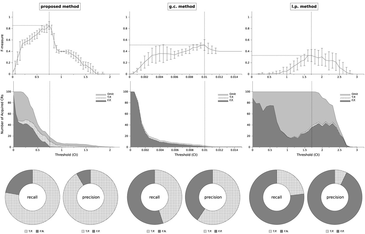
Figure 3. Top: F-measure of the algorithms. Changing acquisition threshold C_T to find $C_T^{\ast }$. It and F* are denoted with vertical and horizontal dotted lines, respectively. Middle: number of acquired CRs, categorized to omitted ones, true positives (T.P.), and false positives (F.P.) Bottom: precision and recall of the methods when $C_T=C_T^{\ast }$, mentioned with the ratio of acquired CRs: true positives and false negatives (F.N.) for recall; true positives and false positives for precision.

Checking the acquired CRs for the g.c. method indicates that it could usually acquire GF, but difficult to acquire GR, OL, and OL2. According to equation (12), the contingency is evaluated among the variables in the g.c. method. Therefore, the averaged dependency of different values of R_k on each value of S_i and A_j is evaluated. However, in GR, OL, and OL2, the averaged dependency would be small, because the dependency only exists among a specific value of R_k on a specific value of S_i and A_j. For example, in OL, the dependency exists only among $R_3^{t+1}=1$, $R_3^t=0$, $S_{\mathit{GR}}^t=1$, and $A_1^t=g_1∕g_2∕g_3$. Therefore, the g.c. method could not acquire them easily, and consequently its F-measure was unable to attain a high value. In the case of the l.p. method, although it acquires many predictable experiences as contingent ones, as mentioned in section 1 and according to equation (8), it could not detect which one is dependent on the state of the caregiver. Therefore, the desired CRs, such as GF and GR, could not be distinguished from the others, and as a result the F-measure of the system is very small.

After detecting $C_T^{\ast }$ and comparing the performance of the methods, we are now able to compare another important factor for the implementation of the system in real-world robots: the speed of the algorithms. Figure 4 shows the speed of acquiring CRs at different levels. We ran the simulation consisting of 30,000 time steps 30 times for each method with $C_T=C_T^{\ast }$, and plotted the average remaining time steps to the end of the simulation, when the CR is acquired. For the g.c. method, which uses the global contingency measure, we judged the CR of a level to be acquired when the set of variables (S_i, A_j, R_k) is determined to be contingent using equation (12). To ensure a fair comparison, in the case of the proposed and l.p. methods, which use a local contingency measure, the level is judged to have been acquired when all of the CRs denoted in the list in section 3.1.3 for each of the levels are obtained by the robot. For example, GF was judged as acquired when the gaze following to the left (g₁), right (g₂), and central (g₃) directions were obtained.

FIGURE 4

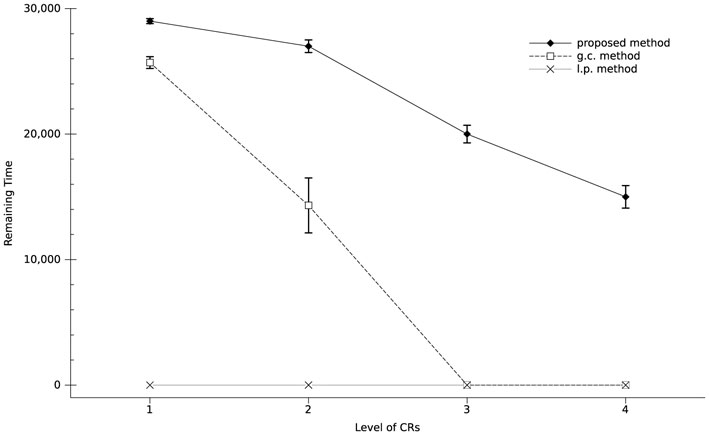
Figure 4. Required time steps for the acquisition of skills in each method. The proposed method is four to eight times faster than the g.c. method.

According to the graph, the proposed mechanism acquired CR with level 1 (i.e., GF) four times faster than the g.c. method, and CR with level 2 (i.e., GR) eight times faster. Furthermore, the proposed method was able to acquire CRs with levels three (OL) and four (OL2) even in shorter time steps than the g.c. method for CRs with level 2, whereas the g.c. method could not acquire CRs with levels 3 and 4. The result of the l.p. method is 0 for all levels of CRs, because it could not acquire all possible CRs denoted in the list in section 3.1.3, for any of the levels. The reason seems to be shown in the middle graph of Figure 3. According to the graph, it acquired many CRs of which most are not true positive, having used full acquisition capacity N_C = 100. Therefore, even for the level of one it could not acquire all of the true positives, i.e., the CRs denoted in the list of GF in section 3.1.3. The reason for the late contingency detection of the g.c. method is the same as that described for Figure 3: evaluating contingency among the variables. Since there is contingency among specific values of the variables, evaluating the average of the contingency among all of the values of the variables leads to the underestimation of the contingency. Therefore, the system needs to gather more experiences until the average exceeds the threshold value C_T, which requires a larger number of time steps to acquire a CR.

Figure 5 shows the effect of uncertainty on the performance of the system. It is implemented by considering wrong data/action for both the perception and motor commands of the robot, because we cannot ignore any of these in a real-world robot. The probability of the uncertainty is defined by the variable η. We ran 100,000 time-step simulations 30 times for different values of η, with $C_T=C_T^{\ast }$. The average of the F-measure over the 30 runs is plotted in Figure 5. As expected, increasing η causes a reduction in the F-measure of the system, for all the methods. Since the contingency is evaluated based on the histogram of the experiences, having wrong data disturbs the histogram and increases the calculation error of the contingencies, which leads the F-measure to be decreased. However, as Figure 5 shows, the F-measure of the proposed method is more than the twice as large as those of the other methods when η < 0.25. Therefore, in real-world implementations, small mistakes in the behavior of the human or the sensors of the robot are expected to be tolerated when our proposed mechanism is used in the implementation.

FIGURE 5

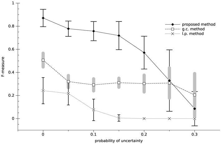
Figure 5. Performance of the systems with uncertainty.

3.2. The Second Experiment

In the previous section, we showed that our system operates faster, finds more complex CRs, and displays a higher resistance against uncertainty compared with the other methods. However, the environment was simplistic: the number of modalities of the robot was small and the contingencies stemmed from a single rule of the caregiver’s response to the robot. As a result, the question as to whether the system would be capable of acquiring social behavior in a more complex environment, which more closely resembles the interactive environment of humans, arose. In this section, we use a more complex environment to examine our proposed mechanism. The number of modalities is increased and the response of the caregiver is designed with multiple rules relying on the different modalities. In this experiment, we set the constant parameters as (C_T, τ) = (0.75, 1.0) base on our experiences.

3.2.1. Experimental Setup

We add a new modality and variables to the robot for this experiment (see Table 2). Specifically, we enable the robot to utter a sound, and to hear the voice of the caregiver. In addition, we enable the robot to recognize the emotion on the face of the caregiver. Thus, A₃ represents the utterance of the robot, u indicates that the robot utters, whereas u_ϕ indicates that it does not. R₄ represents whether the caregiver uttered, whereas R₅ indicates whether the caregiver is smiling.

TABLE 2

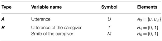
Table 2. Additional variables for the experiment.

3.2.2. Caregiver Model

We increase the behavioral complexity of the caregiver model according to the changes in the variables. In principle, the caregiver behaves in the same way as described in section 3.1.2, but also executes the following additional actions:

1. If the robot uttered to the caregiver after following the gaze of the caregiver, the caregiver responds to the robot by uttering (UU⋅GF-behavior).

2. After the gaze following behavior of the robot, if the robot returned to the caregiver and kept looking at him/her for a while (here, it is one time step), the caregiver utters to the robot (UK⋅GR-behavior).

Note that in this experiment, the caregiver smiles when the robot looks at the caregiver after the GF behavior, in addition to LB-behavior (see section 3.1.2). We denote this with SLB-behavior.

3.2.3. Expected Contingencies

Since new response rules are added to the behavior of the caregiver model (section 3.2.2), the following behavior is expected to be acquired by the robot in addition to that described in section 3.1.3:

• uttering after GF behavior, which would lead the caregiver to respond to the utterance of the robot (GU behavior) and

• keeping the gaze on the caregiver after GR behavior, which would lead the caregiver to utter (KT behavior).

However, a quantitative analysis of the performance of the system, such as in section 3.1.4 is not feasible. This is because there were many parallel causal behavioral actions from the caregiver model in this experiment, and acquisition of one contingency may disturb the acquisition of another one. For example, acquiring the KT behavior may disturb the acquisition of OL behavior, because KT suggests A₁ = g_c as the output a*, whereas OL suggests A₁ = g₁/g₂/g₃. Therefore, instead of performing a quantitative analysis, we inspected the acquired CRs one by one after the simulation to determine what kind of behavior the robot could represent by each of them.

3.2.4. Results and Discussion

We ran the simulation consisting of 10,000 time steps to determine the interaction of the robot with the caregiver model. Table 3 shows all 28 of the CRs acquired by the robot in this experiment, which are classified in 11 behavioral categories (note that in this example, the system acquired 34 experiences as CR, but during the interaction 6 of them were omitted which none of them represented any contingency, and 28 skills were remained). The column labeled “CR Level” indicates the length of the contingency chain of each skill, which is described in section 2.1. The column “Variables” determines the variables of the CRs. In the column “Symbol,” we assigned a symbol to CRs based on the behavior of the robot when it uses the CRs. We use the symbols to indicate the S^π of added CR, in the column “Variables” of Table 3. In “CR Number,” we allocated an ID to each CR. This would enable the value to be used if the CR is the input of another CR. The columns “Input” and “Output” show the input and the output of the sensory-motor mapping of each CR. Furthermore, the value of E(e) when the robot acquired the CR and the predictability Z at the end of the simulation is shown for each CR. Finally, an interpretation of the CR is given based on the functionality in the last column. Below, we explain each behavioral type briefly:

• GF: this behavior, named Gaze Following, enables the robot to follow the gaze of the caregiver when it detects that the caregiver is looking at a point of the table (when C = f₁/f₂/f₃, outputs G = a* = g₁/g₂/g₃). Due to the OR-behavior of the caregiver and infrequent movement of the object (m = 10), using GF leads the robot to (usually) find the object (O^t+1 = r* = 1). Therefore, GF appears to be a social skill for finding the object.

• OP: this behavior, named Object Permanency, enables the robot to keep its gaze along the same direction, when it used GF behavior and detected an object (when GF = 1 and O = 1, outputs G = a* = g₁/g₂/g₃). Due to the infrequent movement of the object (m = 10), using OP leads the robot to (usually) see the object again (O^t+1 = r* = 1). Therefore, OP appears to be a social skill to keep looking at the found object.

• GR: this behavior, named Gaze Return, enables the robot to look at the caregiver when the robot used GF behavior (when GF = 1, outputs G = a* = g_c). Due to the SLB-behavior of the caregiver, using GR leads the robot to detect the smiling face of the caregiver (M^t+1 = r* = 1). Therefore, GR appears to be a social skill for looking back at the caregiver to obtain a prize by smiling, when it succeeded in finding the object (by GF).

• VR: this behavior, named Voice Response, enables the robot to utter a sound when it used GF behavior (when GF = 1, outputs U = a* = u). Due to the UU⋅GF-behavior of the caregiver, using VR leads the robot to detect the vocal response of the caregiver (T^t+1 = r* = 1). Therefore, VR appears to be a social skill for uttering a sound to elicit a vocal response from the caregiver, after the robot succeeded in finding the object (using GF).

• CA: this behavior, named Check Again, enables the robot to look at the previous location of the object when it used VR behavior (when VR = 1, outputs G = a* = g₁/g₂/g₃, where g_i would be the same as that used in GF two time steps before). Due to the infrequent movement of the object (m = 10), using CA leads the robot to (usually) see the object again (O^t+1 = r* = 1). Therefore, CA appears to be a social skill to again verify the existence of the found object in the same place, which is detected in the previous time steps (by GF).

• GU: this behavior, named Get Utterance, enables the robot to keep looking at the caregiver when it used GR behavior (when GR = 1, outputs G = a* = g_c). Due to the UK⋅GR-behavior of the caregiver, using GU leads the robot to detect the utterance of the caregiver (T^t+1 = r* = 1). Therefore, GU appears to be a social skill to elicit an utterance from the caregiver by continuing to look at the caregiver after receiving a smiling prize (by GR).

• KT: this behavior, named Keep Talking, enables the robot to look at the caregiver when it used VR behavior (when VR = 1, outputs G = a* = g_c). Due to the UK⋅GR-behavior of the caregiver and GR behavior of the robot in the previous time step (note that when VR behavior is used, GR behavior would be used simultaneously according to the formerly acquired CRs of the robot), using KT leads the robot to detect the utterance of the caregiver (T^t+1 = r* = 1). Therefore, KT appears to be a social skill in response to the vocal response of the caregiver (due to VR), in which the robot continues looking at the caregiver whereupon the caregiver utters again and which appears to be the ability to induce the caregiver to continue talking to the robot.

• VR4: this behavior, named Vocal Response Lv4, enables the robot to utter a sound when it used CA behavior (when CA = 1, outputs U = a* = u). Due to the UU⋅GF-behavior of the caregiver, using VR4 leads the robot to detect the utterance of the caregiver (T^t+1 = r* = 1). Therefore, VR4 appears to be a social skill to elicit a vocal response from the caregiver, after the robot succeeded in finding the object (using CA).

• OP4: This behavior, named Object Permanency Lv4, enables the robot to maintain its gaze along the same direction, when it used CA behavior and detected (rechecked) an object (when CA = 1 and O = 1, outputs G = a* = g₁/g₂/g₃). Due to the infrequent movement of the object (m = 10), using OP4 leads the robot to (usually) see the object again (O^t+1 = r* = 1). Therefore, OP4 appears to be a social skill to enable continued looking at the rechecked object.

• GR4: this behavior, named Gaze Return Lv4, enables the robot to look at the caregiver when the robot used CA behavior (when CA = 1, outputs G = a* = g_c). Due to the SLB-behavior of the caregiver, using GR4 leads the robot to detect the smiling face of the caregiver (M^t+1 = r* = 1). Therefore, GR4 appears to be a social skill for looking at the caregiver again to obtain a prize by smiling, when it succeeded in finding (rechecking) the object (by CA).

• CA5: this behavior, named Check Again Lv5, enables the robot to look at the previous location of the object when it used VR4 behavior (when VR4 = 1, outputs G = a* = g₁/g₂/g₃, where g_i would be the same as that used in CA two time steps before). Due to the infrequent movement of the object (m = 10), using CA5 leads the robot to (usually) see the object again (O^t+1 = r* = 1). Therefore, CA5 appears to be a social skill to again verify the existence of the found object in the same location detected in the previous time steps (by CA).

TABLE 3

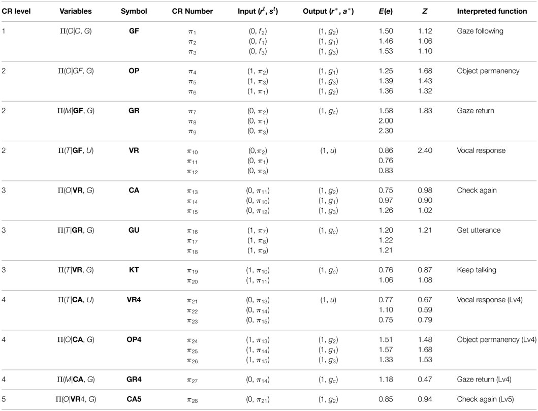
Table 3. Social skills acquired by the robot.

Table 3 indicates that the proposed method was capable of acquiring several social skills based on the response of the caregiver, even in a more complex environment. Compared with the first experiment, social skills with longer sequences, such as CA5 and VR4, are acquired, and more complex interaction between the robot and the caregiver is observed. This suggests that it would be possible to apply our method to real-world interactions between the robot and a human.

To compare the performance of the proposed method under the condition of the second experiment with the other methods, we run 10 independent simulations for each methods, i.e., proposed, g.c., and l.p. methods, where each simulation consists of 10,000 time steps. The average of the number of the acquired CRs (NAC) and the maximum level of the used skill during the interaction [maximum chain length (MCL)] were compared. The average of NAC was 48.6, 1.7, and 93.9 with the SD of 9.1, 0.48, and 6.1 for the proposed, g.c. and l.p. methods, respectively. The average of MCL was 4.2, 1.5, and 2.6 with the SD of 0.42, 0.53, and 0.97 for them, respectively. Larger MCL shows that the robot could interact with the human during longer time sequence, and able to produce more complex behavior. The average of the MCL for the proposed method is larger than the others, which ensures its higher performance even in the complex environment of the second experiment. Although the MCL of the g.c. method is smaller than that of the l.p. method, considering NAC of them could be important. In l.p. method, it is close to 100, i.e., the maximum capacity for the skill acquisition as mentioned in section 3.1.4. It means that the same thing with the result of the first experiment could be occurred for l.p. method, even in the condition of the second experiment. It is considered that the system acquires lots of sensory-motor mapping as CRs, while lots of them do not reflect the condition of the caregiver and are useless for the interaction (see section 3.1.4 for detail). On the contrary, in the case of the g.c. method, the system does not acquire lots of CRs, but NAC seems to be too small, i.e., 1.7. This seems to be similar with the result acquired for the g.c. method in the first experiment (see the middle graph of Figure 3 for the case of the g.c. method). It is difficult to acquire complex skills in case of the g.c. method while there is only one non-complex (i.e., simple) contingent experience set for our experiment, i.e., GF. Therefore, the NAC in the case of g.c method became close to the number of the existing simple experiences, i.e., one.

To more analyze the implication of the result with NAC, we considered a fact that we can identify a part of the combinations that does not reflect any contingencies. For example, the combinations that contain A₂ (hand gesture of the robot) can be identified as non-contingent ones because the caregiver is designed not to produce any responses to the hand gesture of the robot in this experiment. We evaluated RNC, which is the ratio of non-contingent combinations included in the all combinations found in the interaction as a measure implying the accuracy of finding contingencies. In the analysis of this ratio, the found combination is identified as a non-contingent one if a skill satisfies either of the following conditions:

• it contains A₂ (hand gesture of the robot),

• it is level one but is not equal to GF (the only level one contingency exists in our problem setting is GF),

• it is level two but its S variable is not equal to GF (the contingency belongs to two time steps appears only after the execution of GF by the robot in our problem setting), or

• it is level three or higher but its S variable is equal to one of the above (non-contingent) skills.

The average of RNC among the 10 times of the simulations for the proposed, g.c. and l.p. method were equal to 0.17, 0.10, and 0.58 with the SD of 0.09, 0.21, and 0.20, respectively. RNC of the l.p. method is (around two times) larger than that of the proposed method, and it is similar to the result of the first experiment. It means that lots (around 60%) of acquired skills in l.p. method contain non-contingent variables and are useless for the interaction. For case of the g.c. method, RNC is small. However, since it acquires only one or two skills in this problem setting (NAC is equal to 1.7), it does not mean that the robot with the g.c. method succeeds in acquiring contingent complex skills. As a conclusion, the analysis with RNC and NAC for these three methods implies that the similar properties on the accuracy of them appeared in the first experiment, which were treated as an evidence of higher performance of the proposed method, are reproduced in the second experiment, too.

4. Conclusion and Future Work

In this paper, we propose a novel mechanism for the acquisition of social skills utilized in face-to-face interaction between a robot and its human caregiver. We introduced a new contingency evaluation measure that estimates contingencies among the value of the variables utilizing transfer information. Furthermore, we showed that our proposed mechanism improves aspects, such as system precision and recall, contingency chain length, speed, and noise resistance. We additionally examined the feasibility of our proposed system in a more complex environment that more closely resembles real-world interaction of a robot with humans, and showed that the system remained capable of acquiring complex social skills. The resulting fast, accurate, noise tolerant, and complex skill acquisition by the robot encourages us to take the next step, i.e., to implement the system in an actual real-world robot.

However, the skill acquisition threshold C_T was constant in our simulation. In a real-world interaction of a robot with a human, the value of contingency would vary for different types of modalities and different types of interactions. Although we have started to check the performance of the proposed mechanism with a real-world robot, and confirmed the acquisition of even some complex skills by the robot, but in this primitive experiment the parameters including C_T were tuned very carefully and the behavior of the human caregiver were very strict. Therefore, for a natural interaction, a mechanism to adaptively regulate the acquisition threshold through interaction seems to be necessary for the implementation of the proposed method in a real-world robot. It is same for the other prefixed parameters, however, dynamically adjusting all of the parameters by the system seems to be very complex and time-consuming; therefore, discussion about the trade-off of this approach seems to be necessary. Furthermore, to simplify the quantitative analysis of the system performance, RP was considered as a random movement generator in the work described in this paper. However, for a robot in the real world, more complex or human-like RP, such as imitating the caregiver’s motions, or orienting to the ostensive signals like motherese is expected to induce more complex response from the human caregiver. Therefore, such a human-like design of the RP is considered to be one of the design issues to further enhance the performance of the proposed mechanism, which might also promote to establish closer relationship between a human and a robot that keeps providing it with contingent experiences necessary for its open-ended development.

Author Contributions

HM wrote computer code, performed the modeling, analyzed output data, and wrote the paper manuscript. YY supervised the modeling, experimental setup, and data analyses. HI supervised the project.

Conflict of Interest Statement

The authors declare that the research was conducted in the absence of any commercial or financial relationships that could be construed as a potential conflict of interest.

Acknowledgments

This work is supported by MEXT KAKENHI “Constructive Developmental Science” (24119003).

References

Adamson, L. B., and Bakeman, R. (1984). Mothers’ communicative acts: changes during infancy. Infant Behav. Dev. 7, 467–478. doi: 10.1016/S0163-6383(84)80006-5

CrossRef Full Text | Google Scholar

Asada, M., Hosoda, K., Kuniyoshi, Y., Ishiguro, H., Inui, T., Yoshikawa, Y., et al. (2009). Cognitive developmental robotics: a survey. IEEE Trans. Auton. Ment. Dev. 1, 12–34. doi:10.1109/TAMD.2009.2021702

CrossRef Full Text | Google Scholar

Bruner, J., Roy, C., and Ratner, N. (1982). The beginnings of request. Child. Lang. 3, 91–138.

Google Scholar

Butterworth, G., and Jarrett, N. (1991). What minds have in common is space: spatial mechanisms serving joint visual attention in infancy. Br. J. Dev. Psychol. 9, 55–72. doi:10.1111/j.2044-835X.1991.tb00862.x

CrossRef Full Text | Google Scholar

Corkum, V., and Moore, C. (1995). Development of Joint Visual Attention in Infants. New Jersey: Lawrence Erlbaum Associates, Inc.

Google Scholar

Imai, M., Ono, T., and Ishiguro, H. (2003). Physical relation and expression: joint attention for human-robot interaction. IEEE Trans. Ind. Electron. 50, 636–643. doi:10.1109/TIE.2003.814769

CrossRef Full Text | Google Scholar

Kanda, T., Ishiguro, H., Imai, M., and Ono, T. (2004). Development and evaluation of interactive humanoid robots. Proc. IEEE 92, 1839–1850. doi:10.1109/JPROC.2004.835359

CrossRef Full Text | Google Scholar

Kaplan, F., and Hafner, V. V. (2006). The challenges of joint attention. Interact. Stud. 7, 135–169. doi:10.1075/is.7.2.04kap

CrossRef Full Text | Google Scholar

Moore, C., Angelopoulos, M., and Bennett, P. (1997). The role of movement in the development of joint visual attention. Infant Behav. Dev. 20, 83–92. doi:10.1016/S0163-6383(97)90063-1

CrossRef Full Text | Google Scholar

Moore, C., and Dunham, P. (2014). Joint Attention: Its Origins and Role in Development. Hove: Psychology Press.

Google Scholar

Mugan, J., and Kuipers, B. (2012). Autonomous learning of high-level states and actions in continuous environments. IEEE Trans. Auton. Ment. Dev. 4, 70–86. doi:10.1109/TAMD.2011.2160943

CrossRef Full Text | Google Scholar

Nagai, Y., Hosoda, K., Morita, A., and Asada, M. (2003). A constructive model for the development of joint attention. Connect. Sci. 15, 211–229. doi:10.1080/09540090310001655101

CrossRef Full Text | Google Scholar

Oudeyer, P.-Y., Kaplan, F., and Hafner, V. V. (2007). Intrinsic motivation systems for autonomous mental development. IEEE Trans. Evol. Comput. 11, 265–286. doi:10.1109/TEVC.2006.890271

CrossRef Full Text | Google Scholar

Scaife, M., and Bruner, J. S. (1975). The capacity for joint visual attention in the infant. Nature 253, 265–266. doi:10.1038/253265a0

CrossRef Full Text | Google Scholar

Schreiber, T. (2000). Measuring information transfer. Phys. Rev. Lett. 85, 461. doi:10.1103/PhysRevLett.85.461

PubMed Abstract | CrossRef Full Text | Google Scholar

Sumioka, H., Yoshikawa, Y., and Asada, M. (2008). Learning of joint attention from detecting causality based on transfer entropy. J. Robot. Mechatron 20, 378.

Google Scholar

Sumioka, H., Yoshikawa, Y., and Asada, M. (2010). Reproducing interaction contingency toward open-ended development of social actions: case study on joint attention. IEEE Trans. Auton. Ment. Dev. 2, 40–50. doi:10.1109/TAMD.2010.2042167

CrossRef Full Text | Google Scholar

Sumioka, H., Yoshikawa, Y., Morizono, M., and Asada, M. (2013). “Socially developmental robot based on self-induced contingency with multi latencies,” in Advances in Cognitive Neurodynamics (III), ed. Y. Yamaguchi (Dordrecht: Springer), 251–258.

Google Scholar

Triesch, J., Teuscher, C., Deák, G. O., and Carlson, E. (2006). Gaze following: why (not) learn it? Dev. Sci. 9, 125–147. doi:10.1111/j.1467-7687.2006.00470.x

CrossRef Full Text | Google Scholar