Observing the State of Balance with a Single Upper-Body Sensor

1. Introduction

Falls pose a major problem, especially in our aging society. Most falls among the elderly occur during forward walking (24%) and due to incorrect weight shifting (41%) (Robinovitch et al., 2013). Balance dysfunction was found to be a considerable risk factor for falls (Rubenstein, 2006).

Wearable robotic devices could play a role in preventing falls, or at least mitigating their consequences, by providing balance assistance in daily life activities. This would result in increased safety and independence of the elderly. Examples for such systems are the balance-assisting gyroscopic backpack (Li and Vallery, 2012), the hip orthosis (Giovacchini et al., 2014), and airbags to reduce fall injuries (Tamura et al., 2009).

Acceptance of such devices is a critical hurdle, and it relies on the technology being unobtrusive, easy to use, and minimalistic. For example, wearable airbags are mostly contained in just a thin waist belt, and the gyroscopic balance-assisting device is contained in a backpack. Both devices need to rely on sensor data that can be acquired by wearable sensors at the upper body as instrumenting the legs would increase hardware complexity and reduce user comfort in donning and doffing the system.

Standard wearable kinematic sensors are inertial measurement units (IMUs), consisting of accelerometers, gyroscopes, and potentially magnetometers. Such IMUs are commonly used in several fields, not only for real-time fall detection (Kangas et al., 2008), teNyan2008 but also for clinical gait analysis (Goršič et al., 2014; Taborri et al., 2014) or in sport coaching (Exell et al., 2012). IMUs are advantageous in terms of weight, size, energy consumption, and cost. A limitation of IMUs is that they do not allow to directly measure one highly specific predictor for imminent falls: linear velocity in vertical direction. This has proven to be a valuable source of information both in literature (Wu, 2000; Bourke et al., 2008) and in our own experience with the FLOAT rehabilitation robot of Vallery et al. (2013). Despite recent advances in filtering techniques for IMUs (Seel et al., 2014), they cannot deliver linear velocity information without drift or additional assumptions.

Furthermore, most existing fall detection algorithms are based on data-driven or heuristic approaches (Bourke et al., 2008; Nyan et al., 2008a,b) (Kangas et al., 2007), where velocity or acceleration thresholds are used to assess loss of balance. Black-box, data-driven approaches intrinsically rely on large amounts of training data to achieve acceptable specificity (low rate of true positives) and sensitivity (low rate of true negatives) in real-world conditions. Such training data are challenging to obtain. Furthermore, the algorithms need to be specifically configured if more insight is desired besides binary classification of movement as fall or non-fall.

Possibly, the performance of such wearable sensor systems could improve considerably if they were combined with knowledge of nominal human balance behavior. To quantify the state of balance during bipedal gait, multiple definitions have been proposed in literature, both for human locomotion (Hof et al., 2005; Herr and Popovic, 2008; Duclos et al., 2009) and bipedal robots (Goswami and Kallem, 2004; Popovic and Herr, 2005; Pratt and Tedrake, 2006; Wight et al., 2007). What most definitions have in common is that they require at least the position and velocity of the body’s center of mass (CoM) with respect to the center of pressure (CoP), the point of application of the net ground reaction force. These variables are complicated to measure in a wearable application without instrumenting the legs. Moreover, sensors for online measurement usually provide local rather than global information, which is insufficient for fall detection and balance control.

To meet these challenges, we propose to estimate the state of balance by combining local sensor measurements with a simple model of mechanics and control of human gait, in the form of an observer concept.

The choice of model should be as simple as possible to avoid any unnecessary assumptions. Still, the model needs to contain the main features needed to link the state of balance with available sensor information. Particularly, it has to predict orientation of the upper body (which can be measured by IMUs) as well as the base of support and location and velocity of the CoM with respect to it (critical determinants of balance). Many models focus on foot placement only and reduce the upper body to a point mass, such that sensor information from the upper body (like inclination) cannot be integrated (Wisse et al., 2004; Hof, 2008). Also, many models consider double-support phases during gait as instantaneous, which greatly reduces the base of support. This is particularly unrealistic for slow gait of persons with balance impairments, who have extended double-support phases compared to healthy subjects of the same age (Benedetti et al., 1999; Martin et al., 2006), and also for other postural tasks such as sit-to-stand transitions or standing.

As a first step, we aimed for a sagittal-plane model for forward walking on level ground. First, we formulated a set of requirements for such a model (Section 2.2.1), conducted a small survey on available models and their suitability for the observer concept, and we assembled a model based on this analysis (Section 2.2.2). Using simulations, we evaluated the sensitivity of the implemented observer (Section 2.3) to parameter uncertainties (Section 2.4). Finally, we evaluated observer performance using real data from experiments with human subjects (Section 2.5).

2. Materials and Methods

2.1. Notations

Throughout this article, all scalars were written in italic, all vectors in bold italic, and all matrices in bold. Force vectors were denoted with F and moment vectors with M. The global reference frame was denoted as 𝒢 = x, y, z; the body frame with ℬ = u, v, w: u pointed forward, normal to the frontal plane, w pointed upward along the longitudinal axis of the trunk, and v perpendicular to u and w. Mapping between frames is computed as

${}^{\mathcal{G}}\mathit{a}={}^{\mathcal{G}}{\mathbf{R}}_{\mathcal{B}}{}^{\mathcal{B}}\mathit{a}$ (1)

where the rotation matrix ^𝒢R_ℬ maps direction vectors a from the ℬ frame to the 𝒢 frame. In this article, all dynamics are simplified to the sagittal xz plane, so all vectors are reduced to ℝ².

2.2. Dynamic Model

2.2.1. Definition of Requirements

The purpose of this study was quantification of the state of human balance during walking with limited sensor information and under real-time constraints, by means of a model-based observer concept. The first steps were to choose the sensor and an appropriate model for the observer.

As sensor, we chose a minimalistic setup with only a single Inertial Measurement Unit (IMU) at the upper body, near the waist. This is a convenient location for many wearable applications, such as wearable airbags. Furthermore, previous work suggested that accelerometers worn near the waist are effective for preimpact fall detection (Kangas et al., 2008), and that placement near the waist is ergonomic and flexible (Yang and Hsu, 2010).

The model should incorporate the main features of human balance control, while still being observable with the chosen sensor. Three main strategies have been recognized in the literature: the ankle strategy, which counteracts small disturbances during stance and single support; the hip strategy, which utilizes upper-body movement to affect angular momentum in response to slightly larger disturbances; and finally, the stepping strategy or foot placement strategy, which dominates during gait and which copes with disturbances in case ankle and hip strategy do not suffice during stance (Horak, 1987). Trunk control is particularly relevant, because it has been shown that limited trunk motion results in a higher risk for falls, and elderly, who are more prone to falls, often show limited orientation angles and angular velocities (Grabiner et al., 2008). To represent all these strategies, the model needed to have an articulated upper body, trunk, and ankle control, as well as a strategy to place the feet.

We only considered models where experimental evidence existed to confirm their ability to represent human balance strategies.

Finally, the model had to be suitable for a real-time implementation, and it had to include as few parameters as possible, to minimize efforts for the calibration or identification.

2.2.2. Choice of Dynamic Model

To choose a dynamic model, human walking models from the literature were evaluated against our very specific requirements. An overview of these models is given in Table 1. The mechanical models could be categorized into three groups: the linear inverted pendulum (LIP), the spring-loaded inverted pendulum (SLIP), and the multi-body model (MB).

TABLE 1

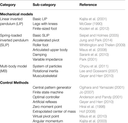
Table 1. Specifications and variations to the three basic mechanical models (linear inverted pendulum, spring-loaded inverted pendulum, and multi-body model) and the two control methods (based on neural principle or mechanical principle).

Even though multibody models have shown very valuable to explain human balance strategies (Herr and Popovic, 2008), the models would not be observable with our chosen extremely limited measurements, and it can therefore not be used.

Due to the constraint of an implementation suitable for real-time application, we excluded some other models, even though they might have the ability to model human-like gait accurately, such as the ones based on optimization techniques (Anderson and Pandy, 2001). We also excluded neuromuscular models, because of the difficulty of determining the many needed muscle-reflex parameters (Geyer and Herr, 2010).

Simplified models with spring legs can reproduce the vertical oscillation of the center of mass, and kinetic and gravitational potential energy resemble human gait (Geyer et al., 2006). Therefore, we chose massless springs as legs.

To represent the upper body in a simple way, we added a single rigid body to the SLIP model, hinged at the hip, as suggested previously by Maus et al. (2010) in the context of Virtual Pivot Point (VPP) control. The VPP hypothesis entails that the resultant ground reaction forces at each foot is always pointed toward a virtual point above the center of mass, by means of controlling hip torques. This way, the upper body mimics a physical pendulum, with the virtual point on the trunk as pivot. As opposed to an inverted pendulum, a hanging pendulum does not require active state feedback control throughout the entire gait cycle. Experimental evidence for this model has been found (Maus et al., 2010). Experiments with models based on the VPP showed high coefficients of determination for predicted ground reaction force direction and predicted whole-body angular momentum (R² > 97.75 and R² > 96%, respectively) for the trunk-attached frame (Maus et al., 2010).

The feature that remained to be added to the VPP model was a foot placement strategy. To this end, the extrapolated center of mass (XCoM) with constant offset control was utilized (Hof et al., 2005). Also for this strategy, experimental evidence exists (Young et al., 2012), although differences in stability margins seem to exist between healthy young subjects, healthy elderly subjects, and elderly fallers (Lugade et al., 2011).

Combining this foot placement strategy with VPP control was expected to result not only in stable behavior of the upper body but also in stable walking behavior. Geometrical definitions of the model are given in Figure 1.

FIGURE 1

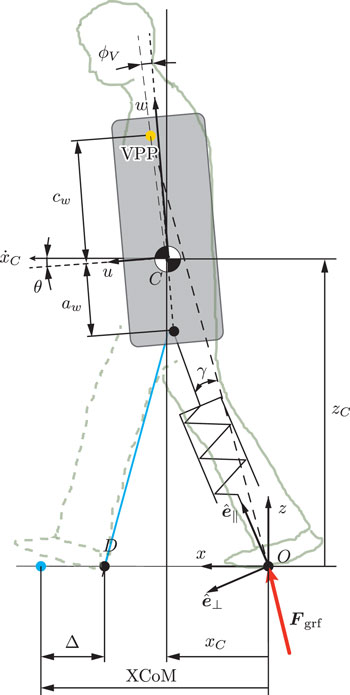
Figure 1. Geometrical representation of Virtual Pendulum Model with virtual pivot point (VPP) control for the upper body (with ground reaction force F_grf) and foot placement with the extrapolated center of mass (XCoM, calculated with the velocity, ${\dot{x}}_C$, of the center of mass).

2.2.3. Movement Generation with the Dynamic Model

2.2.3.1. Assumptions

The equations of motion of the dynamic model were calculated based on the following assumptions:

1. Compliant leg behavior of the human could be modeled with telescopic spring-damper legs; a knee joint did not need to be added to the model.

2. The legs could only be compressed rather than extended, such that the ground reaction force acting on the leg never had a component pointing downwards.

3. Loss of kinetic energy at ground contact was negligible, such that no impact forces occurred and no sudden changes in potential or kinetic energy were present after foot placement; when placing the foot at the ground, the resultant force in direction of the leg equaled zero.

4. Dynamics of the swing leg were negligible; the legs had no mass or inertia, and in swing phase, the legs were at rest length. Accordingly, swing leg dynamics did not appear in the equations of motion.

5. Movement of the center of pressure during single-support phase was negligible; the feet were modeled as point feet, and their positions remained constant throughout stance phase.

Even though the equations of motion of this model could be derived in three dimensions, we neglected the influence of 3D coupling terms and analyzed only a 2D planar model in the sagittal plane.

2.2.3.2. Equations of Motion

All following calculations used the global reference frame 𝒢, the reference frame fixed to the stance foot.

The state vector of the model, q, consisted of 6 state variables: components of the center of mass (CoM) position vector ^𝒢x_C = (x_C, z_C)^T with respect to the origin 𝒪 and of the CoM velocity vector ^𝒢${\dot{\mathit{x}}}_C$ = (${\dot{x}}_C$, ż_C)^T, upper body angular orientation θ, and upper body angular velocity ω = $\dot{\theta }$ as

$\mathit{q}={\left(\begin{array}{cccccc}\hfill x_C\hfill & \hfill z_C\hfill & \hfill \mathrm{\theta }\hfill & \hfill {\dot{x}}_C\hfill & \hfill {ż}_C\hfill & \hfill \mathrm{\omega }\hfill \end{array}\right)}^T.$ (2)

Transformation of a body vector to the global frame was done with a rotation matrix, such as

${}^{\mathcal{G}}{R}_{\mathcal{B}}=\left[\begin{array}{cc}\hfill \cos \left(\mathrm{\theta }\right)\hfill & \hfill \sin \left(\mathrm{\theta }\right)\hfill \\ \hfill -\sin \left(\mathrm{\theta }\right)\hfill & \hfill \cos \left(\mathrm{\theta }\right)\hfill \end{array}\right].$ (3)

These state variables described the configuration and movement of a body, floating in space, with forces and moments acting on it. To stabilize the trunk, the ground reaction force of the leg was directed toward the virtual pivot point (VPP). From a biomechanical perspective, this could be explained with a torque on the hip joint. This ground reaction force F_grf consisted of a component F_|| along the leg (spring and damping forces) with k spring stiffness, d damping coefficient, l₀ rest length of the spring, and l current leg length

$F_{\parallel }=-k\left(l-l_0\right)-d\dot{l}.$ (4)

and a component F_⊥orthogonal to the leg. Thus, using the unit direction vectors e_|| and e_⊥, the angle γ between the leg and the direction of F_grf, and the position vector x_VPP of the VPP with respect to 𝒪, the resultant ground reaction force, F_grf, could be expressed as

${\mathit{F}}_{\text{grf}}=F_{\parallel }{\mathit{e}}_{\parallel }+F_{\perp }{\mathit{e}}_{\perp }=\frac{F_{\parallel }}{\cos \left(\mathrm{\gamma }\right)}\frac{{\mathit{x}}_{\text{VPP}}}{\left|{\mathit{x}}_{\text{VPP}}\right|}.$ (5)

Using Newton–Euler, this resulted in the following equations of motion for single-support phase, with mass m of the upper body, gravitational acceleration g, gravitational force F_g = (0, −mg)^T, and moment of inertia J of the upper body with respect to the CoM (the analysis is restricted to 2D, so the determinant replaces the cross product):

$\left[\begin{array}{c}\hfill m{\ddot{\mathit{x}}}_C\hfill \\ \hfill J\dot{\omega }\hfill \end{array}\right]=\left[\begin{array}{c}\hfill {\mathit{F}}_{\text{grf}}+{\mathit{F}}_g\hfill \\ \hfill -\text{det}\left({\mathit{x}}_C,{\mathit{F}}_{\text{grf}}\right)\hfill \end{array}\right].$ (6)

During double-support phase, the system can be described as a trunk segment with two legs, both in contact with the ground. The equations of motion were similar to those of single support, but one additional force, and moments resulting from this, has to be added: the ground reaction force of the front leg. The point of application of this force was located at the position of foot placement, point D. Ground reaction forces of both legs were directed toward the VPP. These forces together defined the location of the center of pressure which gradually moved from rear to front leg during double-support phase.

The non-linear system was described with the state derivative $\dot{q}$ and the measurement function y

$\dot{\mathit{q}}={\mathit{f}}_j\left(\mathit{q}\right)\text{with}j=1,2$ (7)

$\mathit{y}=\mathit{h}\left(\mathit{q}\right),$ (8)

both functions of the state vector q, where the subscript j denoted either single support (j = 1) or double support (j = 2). These equations could be linearized to get the system matrices A_j as

${\mathbf{A}}_j=\frac{\partial {\mathit{f}}_j\left(\mathit{q}\right)}{\partial \mathit{q}}{\mathrm{|}}_{{\mathit{q}}_k}$ (9)

and output matrix C

$\mathbf{C}=\frac{\partial \mathit{h}\left(\mathit{q}\right)}{\partial \mathit{q}}{\mathrm{|}}_{{\mathit{q}}_k}$ (10)

around a certain state q_k at time instant k.

2.2.3.3. Hybrid Control of Walking

For movement generation, only straight, forward walking on level ground was considered. A simulation of multiple successive steps consisted of two phases: single-support and double-support phase. These two phases were separated by two events: initial contact, IC (at heel-strike), when the swing leg touched the ground; and final contact, FC (at toe-off), when the rear leg left the ground. Both phases were simulated with Heun’s numerical integration method (1000 Hz).

The event functions were based on the assumption of no change in kinetic energy at ground contact. The distance at which the foot was placed, was based on a constant offset to the XCoM. In literature, this was termed constant offset control (Hof, 2008). It has been stated that a constant spatial margin of stability was a possible objective of human walking (Young et al., 2012).

Since the difference between the XCoM of the LIP and the Virtual Pendulum Model was assumed to be negligible, the XCoM derived for the LIP by Hof et al. (2005) was used. For continuous stable walking, the foot needed to be placed posterior to the XCoM. Therefore, initial contact (IC) occurred as soon as the front foot (denoted by index f) could be placed at a point D at a constant offset Δ from the XCoM such that there were zero spring and damping forces, i.e., F_||,f = 0 and XCoM computed with:

$\text{XCoM}=x_C+{\dot{x}}_C\sqrt{\frac{\left|{\mathit{x}}_C\right|}{g}}.$ (11)

The constant offset Δ depended on a given reference step length S_ref, reference step duration T_s,ref, and on the eigenfrequency ω₀ of the pendulum (Hof, 2008):

$\mathrm{\Delta }=\frac{S_{\text{ref}}}{e^{{\mathrm{\omega }}_0{T}_{s,\text{ref}}}+1}.$ (12)

Final contact (FC) occurred when the rear leg (denoted by index r), while extending, regained zero spring and damping forces, i.e., F_||,r = 0 and i ≥ 0.

In double support, the state variables were expressed relative to the foot that first touched the ground (the rear leg). After FC, the origin 𝒪 was moved to the position of the stance foot in single support of the next step.

2.2.4. Observability Analysis

The behavior of the model strongly depended on model parameters and constants, which are given in Table 2. Both spring stiffness, k, [equation (13)] and damping, d, [equation (14)] were computed from a dimensionless value, K and ζ_d, respectively, and other model parameters (mass m, rest length leg l₀, and gravitational constant g):

$k=\frac{K}{l_0}\mathit{mg},$ (13)

$d=2{\mathrm{\zeta }}_d\sqrt{\mathit{km}}.$ (14)

TABLE 2

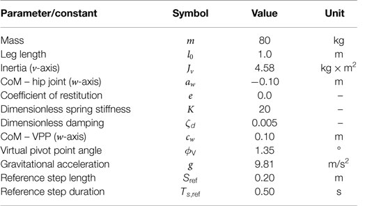
Table 2. Model parameters and constants.

Only angular positions and velocities and linear accelerations were measured; position and velocity of center of mass and leg angle were missing. Only the vertical acceleration ${\ddot{z}}_C$ was used, such that the measurement vector was:

$\mathit{y}={\left(\mathrm{\theta }\mathrm{\omega }{\ddot{z}}_C\right)}^T.$ (15)

To estimate these essential pieces of information, the model needed to be observable. The non-linear equations required an observability check with Lie derivatives, $L_f^i$, which could be calculated with:

$L_{\mathit{f}}^0=\frac{\partial }{\partial \mathit{q}}\mathit{h}$ (16)

$L_{\mathit{f}}^i=\frac{\partial }{\partial \mathit{q}}\left(L_{\mathit{f}}^{i-1}\mathit{f}\right).$ (17)

For local observability, the following holds (with number of states n = 6 and 𝒪 the observability matrix):

$\begin{array}{l}\text{The\hspace{0.17em}system\hspace{0.17em}is\hspace{0.17em}locally\hspace{0.17em}obervable\hspace{0.17em}if:}\text{rank}\left(\mathcal{O}\right)=n\text{with}p<n\hfill \\ \hfill \text{and}\mathcal{O}=\left[\begin{array}{c}{L}_f^0\\ L_f^1\\ ⋮\\ L_f^p\end{array}\right].\end{array}$

This method showed that the observability condition for the dynamic 2D model was fulfilled, if and only if the following conditions held:

$\left\{q_i\mathrm{ϵ}\mathbb{R}|q_i\ne 0\right\}\text{for}i=1,2\dots n.$

We assume that the instants where q_i = 0 were infinitesimally short.

2.3. Observer Design

2.3.1. Observer Concept

The observer needed to estimate human walking behavior. The Virtual Pendulum Model was chosen to approximate this, but it is still, such as human walking, non-linear. A non-linear state estimation technique was thus required.

Yet, the observer needed to be suitable for daily-life applications, such that the state estimates could be utilized for fall detection algorithms and wearable robot control. Therefore, it needed to be possible to run the observer online. This constrained the allowable degree of complexity of the observer type.

It was chosen to use a stochastic state estimation technique, since human walking behavior is stochastic rather than deterministic. We chose a Kalman filter, which is popular due to its relatively straightforward implementation and moderate computational cost.

A well-known example of a Kalman filter is the Unscented Kalman Filter (UKF). This filter does not require derivatives and proved to outperform the commonly applied Extended Kalman Filter (EKF) in terms of accuracy and consistency, without drastically increasing computation time.

The Additive Unscented Kalman Filter is a simple variation to the UKF, with limited amount of sigma points (minimal set of sample points around the mean). With the need for a proof-of-principle, this standard observer for non-linear problems was considered to be appropriate. It should be noted that we do not rule out the possibility of applying other observer types to this method.

2.3.2. Observer Implementation

The observer was implemented offline, but it could also be used online.

The observer was configured to start in a single-support phase. Therefore, estimation started at the instant when the center of mass just passed the stance foot.

First, sets of Sigma-Points were generated with a probability around the prior state estimates. A foot contact detection algorithm defined whether the phase was single or double support. For the simulation, this instant was detected based on the magnitude of the ground reaction forces (as described in Section 2.2.3). Since for the experiment, this kind of information was not available, an existing algorithm published by González et al. (2010), based on accelerometer data, was utilized. At initial contact (IC) detection, foot placement was computed with constant offset control and the XCoM (Section 2.2.3), and stored. The process model for double-support phase was used for the next time step. At the end of the prediction step, a weighted mean was computed from the predicted Sigma-Points, together with a weighted covariance matrix. The weights were divided equally.

After the prediction step, the predicted state estimates had to be corrected by combining predictions with measurements, with process noise and measurement noise matrices as input. The measurements available were upper body angular orientation, upper body angular velocity, and vertical acceleration of the center of mass. The vertical acceleration was integrated to estimate the vertical velocity of the center of mass. A 5th order, high-pass Butterworth filter (normalized cut-off frequency of 0.5) was applied to correct drift. At final contact (FC), the foot placement location (as calculated after IC) was used to move the reference frame to the stance foot in single-support phase. The process model for single support was used subsequently for the next time step.

To tune the observer, simulation data from multiple successive steps were used (40 steps, approximately 16 s). First, the simulation was manually tuned to find an output that converged to a limit cycle. Noise was added for more realistic measurements. Then, the observer parameters, process noise, covariance matrix, and a parameter determining the spread of the sigma-points (γ_s) were set. The measurement noise covariance matrix was determined from the SD of the added noise. Parameters that were found with the tuning process are given in Table 3.

TABLE 3

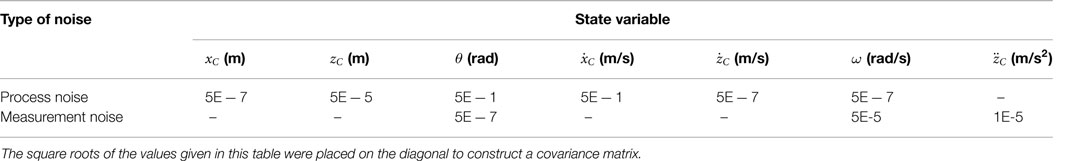
Table 3. Observer parameters, tuned on simulation data.

2.4. Sensitivity Analysis

2.4.1. Evaluation Method

First, the assumptions were verified: whether or not leg length did not exceed rest length, the intersection point of the ground reaction forces was the virtual pivot point (VPP), and the preferred step length and step time were tracked.

After this, observer sensitivity was evaluated, by varying initial conditions and parameters. Values were varied separately while keeping all other conditions and parameters perfect. The effect of the magnitude of these errors on various observer parameters gave an indication of the robustness of the observer.

Event detection was set at the time of initial contact (IC) and final foot contact (FC) (with errors ε_IC and ε_FC). Gait parameters were expected to change depending on type of gait (VPP angle ϕ_V, VPP height c_w, preferred step length s_l, and preferred step duration T_s). All the remaining parameters were model parameters: mass m, leg length l₀, distance from center of mass to hip joint a_w, spring stiffness and damping K and ζ_d, and gravitational acceleration g.

The conditions ranged from perfect values (0% error) as an input, to values deviating largely from the correct ones (100% error), in 5 equally divided steps, both added and subtracted from the perfect values, with measurement noise (Table 4 shows the values considered to be the 100% maximum). The sample frequency was set to 500 Hz. Errors in event detection were based on the mean and SD of errors found in the literature (González et al., 2010).

TABLE 4

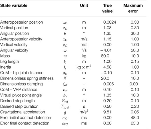
Table 4. True simulation value and maximum errors on initial conditions, model parameters, gait parameters, and event contact detection.

2.4.2. Outcome Measures

The following outcome measures were investigated: root mean squared error (RMSE), convergence time, overshoot, coefficient of determination (R²), and correlation coefficient r.

RMSE of a state variable q_i was calculated with equation (18) over a total of p time steps. To exclude the effect of convergence speed for this evaluation parameter, the initial index k₀ was set at the sample for which t = 10 s, to provide sufficient time to converge. In this equation, ${\widehat{q}}_i$ denotes the estimated, q_i the true state variable.

${\text{RMSE}}_i=\sqrt{\frac{{\sum }_{k=k_0}^p{\left(q_{i,k}-{\widehat{q}}_{i,k}\right)}^2}{p}}$ (18)

Time of convergence was defined as the time from start to the instant that ${\widehat{q}}_{i,k}$ no longer left the interval (q_i,k − ε, q_i,k + ε), with ε a certain set value for that state variable q_i, based on the range of the state variable and what practically was reasonable. The allowed errors were 5 cm on positions, 10 cm on velocities, 3° on angular position, and 5°/s on angular velocity.

Overshoot was defined as the largest difference peak from k = 1 to convergence, with index k = k_c [equation (19)]:

$\underset{1\le k\le k_{\text{c}}}{\max }\sqrt{{\left(q_{i,k}-{\widehat{q}}_{i,k}\right)}^2}.$ (19)

R², coefficient of determination, could be computed with equation (20), with ${\overline{q}}_{i,k}$ the mean value of the data:

$R^2=100\%\cdot \left(1-\frac{{\sum }_{k=k_0}^p{\left({\widehat{q}}_{i,k}-q_{i,k}\right)}^2}{{\sum }_{k=k_0}^p{\left(q_{i,k}-{\overline{q}}_{i,k}\right)}^2}\right).$ (20)

In case of a bias or a gain difference, the correlation coefficient r indicates if the estimates correlates with the true data (ranging between 0, no correlation, 0.3, weak, 0.5, moderate, 0.7, strong, and 1, perfect correlation) and thereby evaluates on phase of walking rather than absolute magnitudes of state variables.

2.5. Experimental Evaluation

2.5.1. Evaluation Method

The performance of the observer was analyzed by comparing the observer outcomes with experimentally measured data. Ethical approval for the experiment was received from the Human Research Ethics Committee, Delft (March, 2015), and the experiment was carried out in accordance to their recommendations. For this study, the data sets of 2 young, healthy subjects were analyzed: 1 male (28 years, 56 kg) and 1 female (24 years, 71 kg). The subjects gave written informed consent.

The set-up consisted of a treadmill with one belt, of which the speed could be varied manually. The test subjects were asked to perform the following tasks on the treadmill for at least 10 s:

1. Low-speed walking (0.56 m/s) (task LW);

2. Normal-speed walking (0.97 m/s) (task NW);

3. High-speed walking (1.35 m/s)¹ (task HW);

4. Normal speed walking with the arms folded in front of the chest (0.97 m/s) (task AW).

Subjects were instructed to walk normally, with the arms free, unless otherwise indicated. Tasks LW and HW were added to validate whether the same observer, tuned on normal speed walking (task NW) could be utilized for different walking speeds. Task AW was added to evaluate the difference in case inertia of swinging arms was absent, since the model neglected arm movements.

Two measurement systems were used: an Inertial Measurement Unit (IMU) and a Motion Capture (MoCap) system. The IMU was attached to the back of the test subjects, at the waist. The MoCap was a 3D, 5-cameras, Motion Capture system (Qualisys Track Manager) to track the movement of the subject, with reflective markers spread according to the placement in Figure 2.

FIGURE 2

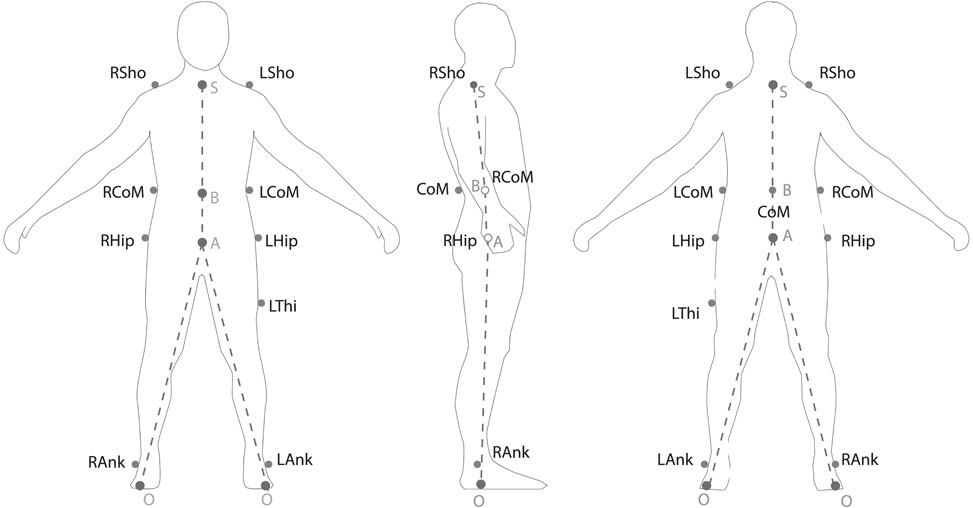
Figure 2. Markers at the subject, used for data analysis (from left to right: front view, right side view, and back view), partially based on guidelines of Carnegie Mellon University. Model shown with dashed line. LThi was used to identify which leg was the left leg. It was assumed that the position of the ankle joint (RAnk and LAnk) coincided with the center of pressure. Note that only the x_C positions rather than the y_C positions were used.

Movement of the markers, providing global position coordinates of points of interest (center of mass, shoulder joints, hip joints, and feet) were tracked with the MoCap system, at 500 Hz. Upper-body angular orientation was estimated from the Inertial Measurement Unit (IMU) data with a Kalman Filter, upper-body angular velocity was measured with the gyros, and linear center of mass acceleration was measured with the accelerometers (1000 Hz, resampled to 500 Hz to match the MoCap measurements). The IMU was calibrated with the z-axis pointing in the opposite direction of gravity, and the x- and y-axes parallel to the ground, using a right-handed system, such that any axis pointing in a direction orthogonal to the vertical gave zero acceleration as an output.

The IMU was placed at the back of the subject’s body in vertical, upright orientation, as close to the position in which the IMU had been calibrated. The alignment was such that the z-axis of the IMU was aligned – as much as possible – with the subject’s upright vertical (longitudinal axis), the x-axis with the direction of walking (sagittal axis), and the y-axis pointing to the left (frontal axis). To calibrate the IMU, such that “zero” angles represented upright standing, the subject was asked to stand as upright as possible, and the “initial” angles from the IMU were recorded. Since most subjects were not able to stand perfectly upright for the short period of time, the measured initial angles varied approximately 3°. The Euler angles were found by calculating the corrected rotation matrix with measured angles (at each time instant) and the (constant) initial angles. A rotation order 1-2-3, from body to global frame, was used (rotating around the body’s x-axis with ϕ, about the rotated y-axis with θ, and around the rotated z-axis with ψ). The calculated Euler angle θ obtained from the IMU data was fed into the observer.

During a trial, after IMU data recording had started, the MoCap recordings were started as well, and stopped after approximately 10 s. With the start and the end of the MoCap recordings, a trigger was sent to the computer that recorded IMU data, such that only the IMU data in between the start and end triggers of the MoCap were saved, and IMU and MoCap recordings were synchronized.

2.5.2. Data Processing

Each dataset (of 10 s) was cut in two, such that per task, two datasets of each 5 s were obtained (labeled, e.g., LW1 for the first 5 s, LW2 for the second 5 s of low-speed walking). The observer was configured to start in single-support phase. Therefore, the start of each dataset was set at the instant when the MoCap recordings of the position of the center of mass just passed the MoCap recording of the position of the stance foot.

After the IMU was calibrated for upright stance, the instants of initial and final foot contact were estimated with the available data from the IMU. The use of accelerometers in combination with gyroscopes has been accepted for online gait event detection. An offline approach, which theoretically could be implemented online, was used. It was based on the approach by González et al. (2010), who showed that initial and final contact events (IC and FC) could be detected from lower trunk accelerations and heuristics, without false positives or false negatives, with an error of 13 ± 35 and 9 ± 54 ms for IC and FC, respectively. Although considerable delays were present (117 ± 39 ms for IC and 34 ± 72 ms for FC), it was suggested these could be reduced by applying a different filter, so that further research could lead to an accurate algorithm for real-time gait event detection (González et al., 2010).

The MoCap data, which returned global position coordinates of each marker, needed to be processed to find the state variables as defined in the model: position and velocity of the center of mass with respect to the stance foot in single support, and to the foot of the rear leg in double support. It was assumed the anteroposterior coordinate of the center of pressure of each foot in contact with the ground always coincided with the marker placed at the ankle joint, the vertical coordinate was assumed to be zero. In other words, the foot was assumed to be a point foot.

The markers were labeled in Qualisys Track Manager. In case a marker disappeared, and the gap did not exceed 200 samples (500 Hz), gaps were filled with a polynomial. Orientation of the upper body for yaw motion, required to extract the anteroposterior coordinates, was based on the direction of the vector from marker LCoM to RCoM or from LSho to RSho, depending on the availability of MoCap data. Anatomical landmarks were used to find points of interest. Hip joint (point A) and shoulder (point S) were defined by the midpoint of the left and right markers of hip and shoulders, respectively. The center of mass (point B) was defined to coincide with the midpoint of markers LCoM and RCoM.² The inclination angle of the upper body was defined by the orientation of the vector from hip joint to shoulder (point A to S in Figure 2). Linear and angular velocities were calculated from the position vectors with the central difference method and filtered with a Butterworth low-pass filter of 50 Hz to filter out noise. For the linear velocity in anteroposterior direction, the central difference method was applied to the absolute position data, and the constant velocity of the treadmill was added to the computed velocity.

The initial conditions for each task as input to the observer were set to the initial conditions found with MoCap and IMU, plus errors that were set to −5 cm for anteroposterior and vertical position, −5 and 5 cm/s for anteroposterior and vertical velocities, respectively, 2.9° for orientation, and 5.7°/s for angular velocity.

Model and observer parameters were tuned with data from the first 5 s of task NW (normal speed walking), task NW1, with the objective of minimizing the error between estimates and measurements, assuming time instants of IC and FC were known without delay. A first guess of the model parameters was done based on information from the MoCap data, values found in the literature for stiffness and damping (Zhang et al., 2000) and the location of the virtual pivot point (VPP) (Gruben and Boehm, 2012). Measurement noise covariance was found from the SD of constant output IMU data. Remaining observer parameters were manually tuned with trial and error, starting with a similar covariance matrix as found by tuning the observer on simulation data.

The independent variables were treadmill speed and type of gait (arms swinging naturally or arms folded in front of the chest). It was hypothesized that these independent variables did not affect the parameters that were tuned, except for the VPP angle ϕ_V, desired step length S_ref, and desired step time T_{s, ref}. Model and observer parameters from normal speed walking task NW1 were applied to all other tasks, while only tuning ϕ_V for a change in speed and adapting S_ref and T_{s, ref} (LW: 0.20 m and 0.70 s, NW and AW: 0.25 m for subject 1, 0.10 m for subject 2, and 0.55 s, HW: 0.3 m and 0.40 s).

2.5.3. Outcome Measures

Three metrics were defined to evaluate observer performance: the root mean squared deviation (RMSD) between the two methods, correlation coefficient r and the coefficient of determination R² (variance explained). To avoid calculation of metrics before convergence and thereby distort the results, an ample convergence time of 2 s was assumed. On the one hand, the two methods to be compared were MoCap measurements and, on the other hand, model-based estimates from the observer, using IMU data.

The results were visualized in a figure, showing mean, 1 SD (σ_D), and a 95% confidence interval [3.182 SEM (σ_M), ${\sigma }_{\mathrm{M}}=\frac{{\sigma }_{\mathrm{D}}}{\sqrt{N}}$ with N the sample size; based on a two-way repeated measures ANOVA with the limited amount of subjects, different types of tasks and different time instants, giving 3 degrees of freedom] and raw data points of RMSD. This type of visualization was chosen because of the limited amount of data points. Non-overlapping confidence intervals indicated a significant difference between the separate tasks, with p = 0.05.

3. Results

3.1. Sensitivity Results

The minimum and maximum values of the outcome measures are given in Table 5, with an input error of 60% of the maximum set error. From this table, it could be understood which variables negatively affected which state variables the least and which did this the most. Also, the magnitudes of the metrics gave an indication of the quality of the best and worst estimates.

TABLE 5

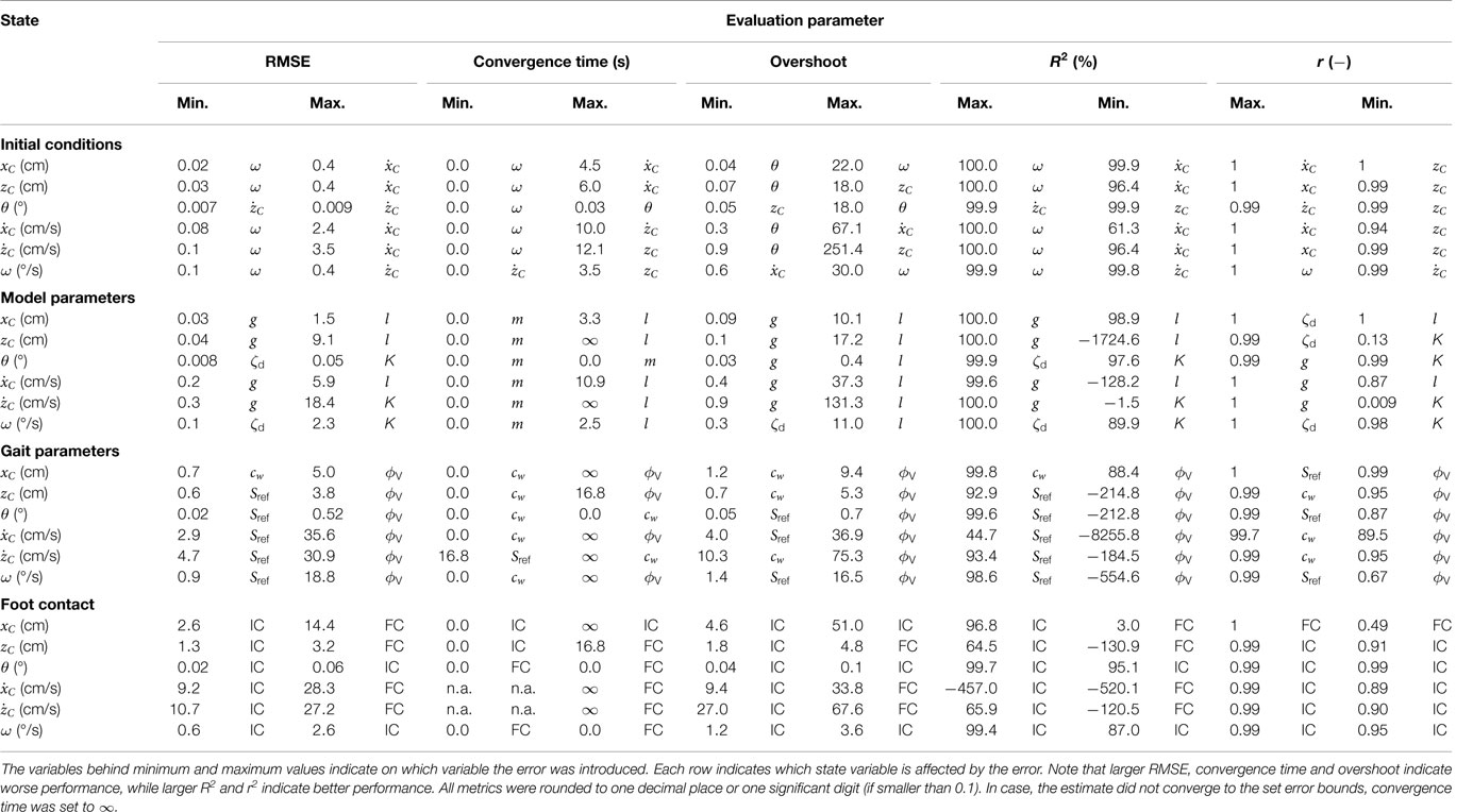
Table 5. Minimum and maximum values of evaluation parameters, with input errors of 60% of the maximum set error given in Table 4, both subtracted and added from the perfect values.

3.2. Performance Results

The behavior of the tuned observer over time of subjects 1 and 2 is visualized in Figures 3 and 4, showing measurements of MoCap and IMU and observer estimates of task NW2, normal speed walking (0.69 < r < 0.93, 0.3% < R² < 77% for subject 1, 0.28 < r < 0.98, −1% < R² < 67% for subject 2).

FIGURE 3

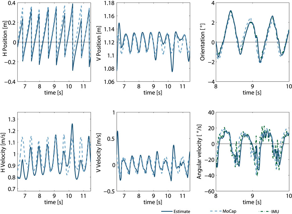
Figure 3. Subject 1. Observer estimates against IMU and MoCap data, second trial of normal walking NW (tuned on first trial of normal walking). Error in initial conditions: 5 cm on CoM position, 2.9° on upper body orientation, 5 cm/s on CoM velocity and 5.7°/s on upper body angular velocity. The time window of orientation and angular velocity outcomes was reduced for better visibility.

FIGURE 4

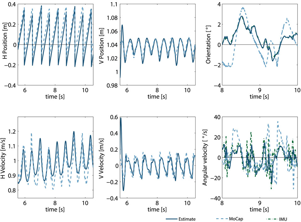
Figure 4. Subject 2. Observer estimates against IMU and MoCap data, second trial of normal walking NW (tuned on first trial of normal walking). Error in initial conditions: 5 cm on CoM position, 2.9° on upper body orientation, 5 cm/s on CoM velocity, and 5.7°/s on upper body angular velocity. The time window of orientation and angular velocity outcomes was reduced for better visibility.

A plot showing RMSD, mean, SD, and 3.182 SEM (95% confidence interval) of all trials per task together is given in Figure 5.

FIGURE 5

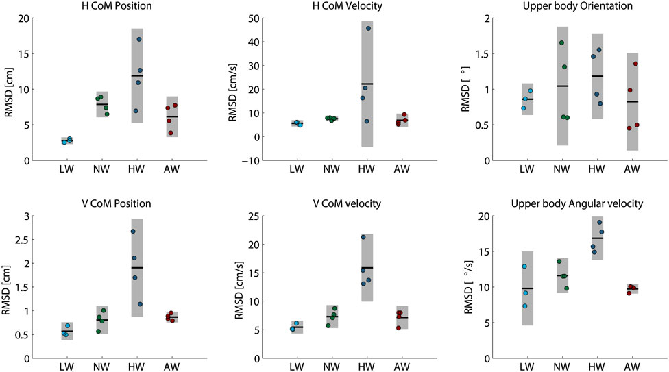
Figure 5. RMSD of different speeds (estimates and MoCap data). Raw data, together with means, spread over a 95% confidence interval (3.182 SEM, gray area) and 1 SD (small black areas at the ends of the gray area), shown per task. Note the difference in scale of y-axes.

The same was done for r correlation coefficient and R² coefficients of determination, for each task and each subject, in Figures 6 and 7, respectively.

FIGURE 6

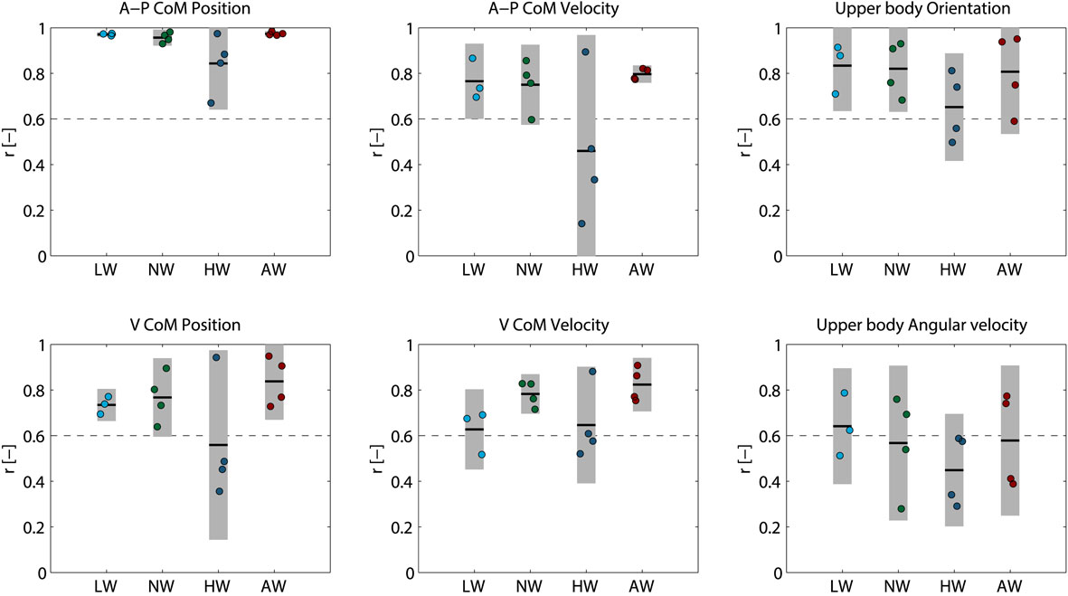
Figure 6. Correlation coefficients r of different speeds (estimates and MoCap data). Raw data, together with means, spread over a 95% confidence interval (3.182 SEM, gray area) and 1 SD (small black areas at the ends of the gray area). The dashed line indicates r = 0.60, a value above which the correlation is preferred.

FIGURE 7

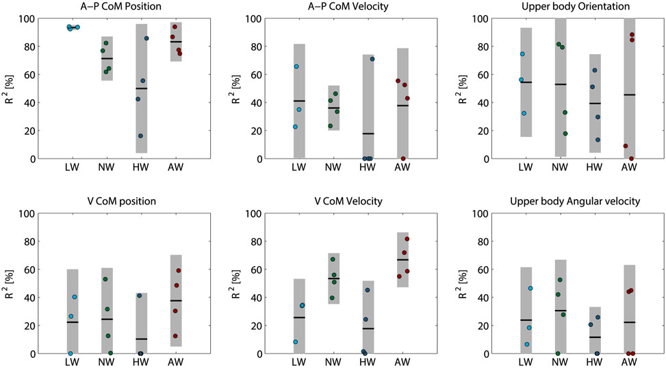
Figure 7. Coefficients of determination R² of different speeds (estimates and MoCap data). Raw data, together with means, spread over a 95% confidence interval (3.182 SEM, gray area) and 1 SD (small black areas at the ends of the gray area). All negative R² values were scaled to 0 for this plot, to improve visibility of the spread of positive R² values. True R² values can be found in Table 6.

TABLE 6

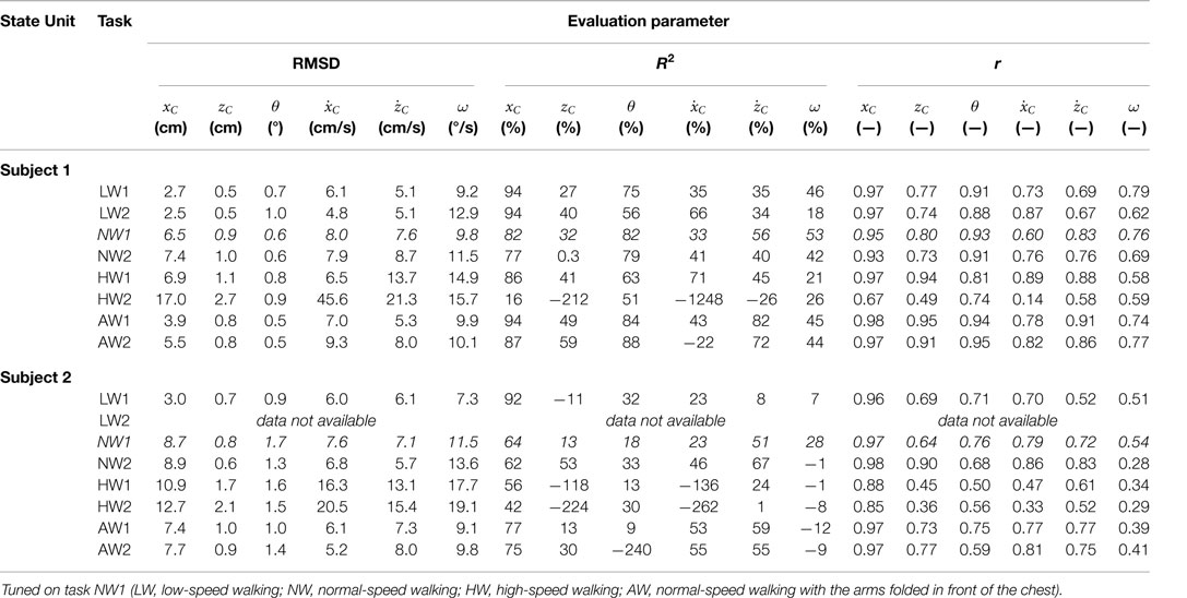
Table 6. Coefficients of determination R² and correlation coefficients r of observer estimates of experimental trials, compared to MoCap measurements.

Each metric (RMSD, R², and r), for both subjects, each task, and each state variables separately can be found in Table 6.

4. Discussion

4.1. Sensitivity

To verify the working principle of the observer, the dynamic model was simulated to evaluate model behavior, and the sensitivity of the observer was tested with simulation results. It followed that the observer converged when inducing errors on initial conditions. The observer was sensitive to errors in specific model parameters, gait parameters, and time of foot contact.

Changing initial conditions did not highly affect the RMSE of the estimates. Maximum errors on CoM position, after 10 s, did not exceed 1 cm; on linear CoM velocity 7 cm/s; on upper-body orientation 0.02° and on upper body angular velocity 0.5°/s. R² variance explained and r correlation coefficient were hardly affected either, except for anteroposterior CoM velocity (R² = 61.3% and r = 0.94% for a 60% error on anteroposterior CoM velocity). Large errors in initial conditions, however, have an effect on convergence speed and overshoot: CoM velocities needed more than 10 s to converge, and overshoot highly increased (up to 2.5 m for ż_C with a 60% error on z_C). Overall, mainly errors in upper-body orientation (θ) and upper-body angular velocity (ω) had a minor effect on the performance metrics, while vertical CoM position (z_C) and CoM velocities (${\dot{x}}_C$ and ż_C) had the largest effect. Both θ and ω were hardly affected by errors in any state variables. This was expected, since these state variables were measured.

The observer was sensitive to various parameter errors. The two model parameters with the largest effects were leg length and spring stiffness. These parameters did not only induce larger RMSE (15 cm error on anteroposterior CoM position (x_C) and 18.4 cm/s on vertical CoM velocity (ż_C) for 60% error), longer convergence times, and larger overshoot but also resulted in a bias, such that the estimate did not converge and the coefficient of determination assumed large negative values (−1724.6% and −128.2% for vertical CoM position (z_C) and anteroposterior CoM velocity (${\dot{x}}_C$) respectively, with a 60% error). This bias was present in the z_C-coordinate as a result of the hip position parameter. Leg length and hip position were both parameters that could be estimated quite accurately, assuming the center of mass was positioned at the waist. Spring stiffness however proved to be more cumbersome: not only was the spring stiffness of the human leg difficult to estimate, it was also unclear how the actual leg stiffness of the human related to the spring stiffness in the Virtual Pendulum Model. The state variables most sensitive to this type of errors, were anteroposterior CoM position x_C and linear, vertical CoM velocity ż_C.

One of the model parameters that depended on type of gait (gait parameters) highly affected the behavior of the observer: the VPP angle ϕ_V, with RMSE errors of 35.6 cm/s for anteroposterior CoM velocity (${\dot{x}}_C$), 30.9 cm/s on vertical CoM velocity (ż_C), even 18.8°/s on upper body angular velocity (ω), and a mean R² of −1555.7 for 60% error. It was suggested that the VPP angle was related to the speed of walking: a larger positive VPP angle increased the average speed, while zero angle or a small negative VPP angle decreased the speed (Kenwright et al., 2011). Possibly, this parameter should be adapted online, for instance based on heuristics, in order to obtain an observer that could cope with speed changes.

Finally, time of foot contact detection highly influenced the estimates: 14.4 cm RMSE on anteroposterior CoM position (x_C), 28.3 cm/s on anteroposterior CoM velocity ${\dot{x}}_C$, and 27.2 cm/s on vertical CoM velocity ż_C for 60% error. In most cases, especially final contact (FC) detection was of importance. Additional sensors on the feet or the event detection algorithm should be robust and accurate to avoid errors in foot contact detection. Also, the delay should be minimized.

Overall, the measurements (upper-body orientation θ and upper-body angular velocity ω) were least influenced by input errors. Anteroposterior CoM position (x_C) was sensitive to errors, especially to time of foot contact. The difficulty of this state variable resided in the fact that it depended on the previous value, which resulted in cumulative errors that kept increasing.

A limitation of this verification method was the dependency on one simulation set. Many limit cycles could be found, of which one would be more stable than the other (Maus et al., 2008), and of which one would correspond better to experimental human walking data than the other.

In case the parameters leg length, hip joint position (VPP) angle, spring stiffness, and time of FC were estimated incorrectly, the estimates became unreliable. Using a less versatile model, such as the LIP, or simply predicting the mean, might in these cases be preferred. The parameters that had little effect on the evaluation parameters were gravitational constant, damping, mass, desired step length, and height of VPP. Based on these simulation results, the Additive Unscented Kalman Filter seems a feasible option for estimating the state of balance.

4.2. Performance

A human walking experiment on a treadmill was conducted to validate the hypothesized human walking strategy. This experiment showed that it was possible to predict the state of balance in agreement with Motion Capture (MoCap) measurements, with the proposed Virtual Pendulum Model and the Extrapolated Center of Mass. Convergence of the estimates of a representative trial is shown in Figure 3.

The quality of the estimates differed per trial: The low-speed walking task LW and the normal-speed walking tasks NW and AW (arms folded in front of the chest) gave on average lower RMSD values, higher coefficients of determination, R² and higher correlation coefficients r compared to the high-speed walking task HW. A possible explanation could be the violation of model assumptions with higher velocities: negligible dynamics of the swing leg, negligible movement of the center of pressure, or the assumption of no impact forces at foot contact.

Mean RMSD values did not exceed (approximately) 13 cm for anteroposterior (A–P) CoM position, 2 cm for vertical (V) CoM position, 22 cm/s for A–P CoM velocity (0.56–1.35 m/s), 17 cm/s for V CoM velocity, 1.2° for upper-body orientation, and 17°/s for upper-body angular velocity. A trend was observed in Figure 5: RMSD values seemed to increase with increasing velocity. The largest RMSD values were found for HW, even indicating a significant difference for vertical CoM position and velocity, and upper body angular velocity. One of the fall indicators, the vertical velocity of the center of mass, of which the threshold was set at −1.3 m/s by Bourke et al. (2008), showed RMSD values that were considerably lower (0.05–0.20 m/s) than the threshold value. The RMSD values found with a 95% confidence interval of vertical CoM position and upper body orientation were, due to their small magnitude, considered to be practically not important.

The behavior of the human was highly correlated with the behavior of the Virtual Pendulum Model: The mean correlation coefficient r was 0.76, 0.77, 0.60, and 0.80 for LW, NW, HW, and AW, respectively. Especially A–P CoM position x_C and upper-body orientation θ showed high correlation coefficients. Mean r of the LW, NW, and AW tasks were above 0.60 for all state variables, except for upper-body angular velocity θ of NW and AW (r ≈ 0.55), while estimates of HW showed a less strong correlation.

Interestingly, the coefficient of determination R² implied a less positive conclusion than implied by correlation coefficient r: mean R² was 47, 58, 46, and 54% for LW, NW, HW, and AW, respectively. In some cases, especially for vertical CoM position z_C and A–P CoM velocity ${\dot{x}}_C$, R² assumed negative values, possibly due to little variation in z_C data. Only for x_C and θ, more than, on average, 40% of the variance in the measurements could be explained with the model.

These findings showed that this controlled mechanical model was, both in theory and in practice, observable with only the limited, local available measurements; local kinematic information of the upper body was sufficient to acquire information on the position of the feet, and on global information of the center of mass. With this proof of principle, the model can be fine-tuned to improve the quality of the estimates, such that it can be applied in wearable robots.

These findings also support the theory of a stabilizing force direction pattern in the sagittal plane. While previous studies validated the existence of the virtual pivot point (VPP) (Maus et al., 2008, 2010; Gruben and Boehm, 2012), this study focused on exploiting the concept to make enhanced predictions. Herewith, two lines of research were combined: human movement theory (Anderson and Pandy, 2001; Geyer and Herr, 2010) and observer application (Lebastard et al., 2004; Yun and Bachmann, 2006; Czarnetzki et al., 2009). Moreover, even though the XCoM of a spring legged model does not exactly coincide with the XCoM of a linear inverted pendulum (LIP) (Van der Geld, 2012), from the limited RMSD in A–P CoM position, it could be concluded the assumption of using LIP XCoM was valid.

It should be noted that the validation measurements of the MoCap data differed from the IMU data, such that the difference between the true error and the estimated deviation was unknown. It was hypothesized that the agreement of MoCap data and IMU for upper-body orientation and upper-body angular velocity was correlated with the agreement of CoM position and velocity estimates with MoCap measurements. However, more data need to be processed to draw a significant conclusion.

One limitation of this study concerned assumptions on foot contact. Particularly, the model neglected a moving center of pressure from heel strike to toe-off, and it assumed zero delay in foot contact detection.

Another limitation concerns manual tuning of gait parameters for different walking tasks, which is disadvantageous for online estimation. The magnitudes of the entries in the process noise covariance matrix were difficult to find. Although a satisfactory result was found, it is very likely that this result was suboptimal. Because of the multitude of parameters, it was expected that optimization techniques would be computationally too expensive and that local minima rather than the global minimum would be found.

A large limitation concerns the type of movements that were investigated. Our experimental trials included walking at three different speeds, but other activities of daily living were not considered. The effect of different activities with a varying rate of angular momentum on the VPP was not investigated, such that no conclusions regarding the performance of the observer in activities other than forward walking could be drawn. Specifically prior to a fall, the rate of change of angular momentum can be large, which could potentially have a negative effect on observer performance. Therefore, for further research, it is suggested to include other activities of daily living and perturbed walking data.

Furthermore, our calibration routine is not practical outside of a laboratory environment and with subjects with balance impairments. In a clinical environment, faster and easier algorithms and protocols should be employed, for example as in Palermo et al. (2014a,b) and Taborri et al. (2014).

It should be noted that in theory, the same method as presented here could be utilized for frontal-plane evaluation and extended to 3D evaluation. It is suggested to investigate if 3D application is possible for real time use and significantly better than using two decoupled 2D models (sagittal plane and frontal plane). Also, it would be interesting to explore how the position of the VPP depends on anthropomorphic measures, age, or type of daily life activity.

How the human walks and which underlying fundamental principles govern human walking is a comprehensive and complex topic. Further research is required for optimization of the observer based on these concepts, such that it can successfully be applied in wearable robotic controllers. Many other models exist and could be investigated in a similar observer concept.

5. Conclusion

The goal of this study was to quantify balance with measurements on the upper body. It was hypothesized that this could be done with the Virtual Pendulum Model as dynamic model, which used the virtual pivot (VPP) concept, combined with the Extrapolated Center of Mass, XCoM, and the Additive Unscented Kalman Filter as observer.

First, the observer was tested on simulation data and showed to converge, with varying initial conditions. The observer was especially sensitive to errors in leg length, hip joint position, VPP angle, spring stiffness, and time of final contact. Other parameters, such as the gravitational constant, damping coefficient, mass, and desired step length, had little effect on the quality of the estimates. A limitation of the observer was the high sensitivity to model parameters and foot contact detection, and the amount of observer parameters that had to be tuned.

Second, the observer was evaluated with experimental data (using a Motion Capture system and an existing foot detection algorithm), showing that, if properly tuned and if instants of foot contact were estimated correctly, the observer gave a satisfactory estimate of human walking. Position of the center of mass could be estimated with an accuracy of less than 13 cm, and congruence of the model with real data was characterized by a coefficient of determination around 50%.

With this study, it was shown that the VPP and the XCoM seem to be valuable principles that can effectively be used in combination with the Additive Unscented Kalman Filter to make predictions on human balance.

Author Contributions

CP contributed to the conception of the work, acquisition, analysis and interpretation of data, and drafted the work. DL contributed to the conception of the work and interpretation of the data, revised the work critically, and was the daily supervisor of the corresponding author, CP. DS contributed to acquisition of the data and provided feedback on the work. HV contributed to the conception of the work, analysis and interpretation of the data, and revised the work critically. Furthermore, all authors gave final approval for the version to be published and agreed to be accountable for all aspects of the work.

Conflict of Interest Statement

The authors declare that the research was conducted in the absence of any commercial or financial relationships that could be construed as a potential conflict of interest.

Acknowledgments

This research was supported by the U.S. Department of Health and Human Services information (HHS Grant Award Number: 90RE5010-01-01, HHS CFDA Number: 93.433), and by the Marie-Curie career integration grant PCIG13-GA-2013-618899. The authors would like to thank D. van der Pool and M. Wisse for their valuable feedback on the work, and R. di Pace and L. Grande for their support with the experiment.

Footnotes

1. ^The treadmill speed indicated at the display was validated with the MoCap data of the foot. For low and normal velocities, the average speed of the foot corresponded to the speed indicated at the treadmill. However, for high velocities, a drift was observed. For tasks HW, instead of 1.4 m/s, which was the treadmill input, 1.35 m/s was estimated to be the actual velocity according to the processed MoCap data.
2. ^For some datasets, the RCoM marker was not visible for most of the time and did therefore not provide sufficient information. In this case, the vector from left-to-right shoulder was projected to the center of mass plane. The intersection of this vector and the vector orthogonal to it, starting in CoM, defined the center of mass.

References

Anderson, F. C., and Pandy, M. G. (2001). Dynamic optimization of human walking. J. Biomech. Eng. 123, 381–390. doi:10.1115/1.1392310

PubMed Abstract | CrossRef Full Text | Google Scholar

Benedetti, M., Piperno, R., Simoncini, L., Bonato, P., Tonini, A., and Giannini, S. (1999). Gait abnormalities in minimally impaired multiple sclerosis patients. Mult. Scler. 5, 363–368. doi:10.1177/135245859900500510

PubMed Abstract | CrossRef Full Text | Google Scholar

Bourke, A., Odonovan, K., and Olaighin, G. (2008). The identification of vertical velocity profiles using an inertial sensor to investigate pre-impact detection of falls. Med. Eng. Phys. 30, 937–946. doi:10.1016/j.medengphy.2007.12.003

PubMed Abstract | CrossRef Full Text | Google Scholar

Chyou, T., Liddell, G., and Paulin, M. (2011). An upper-body can improve the stability and efficiency of passive dynamic walking. J. Theor. Biol. 285, 126–135. doi:10.1016/j.jtbi.2011.06.032

PubMed Abstract | CrossRef Full Text | Google Scholar

Czarnetzki, S., Kerner, S., and Urbann, O. (2009). Observer-based dynamic walking control for biped robots. Rob. Auton. Syst. 57, 839–845. doi:10.1016/j.robot.2009.03.007

CrossRef Full Text | Google Scholar

Duclos, C., Desjardins, P., Nadeau, S., Delisle, A., Gravel, D., Brouwer, B., et al. (2009). Destabilizing and stabilizing forces to assess equilibrium during everyday activities. J. Biomech. 42, 379–382. doi:10.1016/j.jbiomech.2008.11.007

PubMed Abstract | CrossRef Full Text | Google Scholar

Exell, T. A., Gittoes, M., Irwin, G., and Kerwinb, D. (2012). Gait asymmetry: composite scores for mechanical analyses of sprint running. J. Biomech. 45, 1108–1111. doi:10.1016/j.jbiomech.2012.01.007

PubMed Abstract | CrossRef Full Text | Google Scholar

Geyer, H., and Herr, H. (2010). A muscle-reflex model that encodes principles of legged mechanics produces human walking dynamics and muscle activities. IEEE Trans. Neural. Syst. Rehabil. Eng. 18, 263–273. doi:10.1109/TNSRE.2010.2047592

PubMed Abstract | CrossRef Full Text | Google Scholar

Geyer, H., Seyfarth, A., and Blickhan, R. (2006). Compliant leg behaviour explains basic dynamics of walking and running. Proc. Biol. Sci. 273, 2861–2867. doi:10.1098/rspb.2006.3637

PubMed Abstract | CrossRef Full Text | Google Scholar

Giovacchini, F., Vannetti, F., Fantozzi, M., Cempini, M., Cortese, M., Parri, A., et al. (2014). A light-weight active orthosis for hip movement assistance. Rob. Auton. Syst. 73, 123–134. doi:10.1016/j.robot.2014.08.015

CrossRef Full Text | Google Scholar

González, R. C., López, A. M., Rodriguez-Uría, J., Álvarez, D., and Alvarez, J. C. (2010). Real-time gait event detection for normal subjects from lower trunk accelerations. Gait Posture 31, 322–325. doi:10.1016/j.gaitpost.2009.11.014

PubMed Abstract | CrossRef Full Text | Google Scholar

Goršič, M., Kamnik, R., Ambroi, L., Vitiello, N., Lefeber, D., Pasquini, G., et al. (2014). Online phase detection using wearable sensors for walking with a robotic prosthesis. Sensors 14, 2776–2794. doi:10.3390/s140202776

CrossRef Full Text | Google Scholar

Goswami, A., and Kallem, V. (2004). “Rate of change of angular momentum and balance maintenance of biped robots,” in Robotics and Automation, 2004. Proceedings. ICRA’04. 2004 IEEE International Conference On, Vol. 4 (New Orleans, LA: IEEE), 3785–3790.

Google Scholar

Grabiner, M. D., Donovan, S., Bareither, M. L., Marone, J. R., Hamstra-Wright, K., Gatts, S., et al. (2008). Trunk kinematics and fall risk of older adults: translating biomechanical results to the clinic. J. Electromyogr. Kinesiol. 18, 197–204. doi:10.1016/j.jelekin.2007.06.009

PubMed Abstract | CrossRef Full Text | Google Scholar

Gruben, K. G., and Boehm, W. L. (2012). Force direction pattern stabilizes sagittal plane mechanics of human walking. Hum. Mov. Sci. 31, 649–659. doi:10.1016/j.humov.2011.07.006

PubMed Abstract | CrossRef Full Text | Google Scholar

Herr, H., and Popovic, M. (2008). Angular momentum in human walking. J. Exp. Biol. 211(Pt 4), 467–481. doi:10.1242/jeb.008573

PubMed Abstract | CrossRef Full Text | Google Scholar

Hirai, K., Hirose, M., Haikawa, Y., and Takenaka, T. (1998). “The development of honda humanoid robot,” in Robotics and Automation, 1998. Proceedings. 1998 IEEE International Conference On, Vol. 2 (Leuven: IEEE), 1321–1326.

Google Scholar

Hof, A., Gazendam, M., and Sinke, W. (2005). The condition for dynamic stability. J. Biomech. 38, 1–8. doi:10.1016/j.jbiomech.2004.03.025

PubMed Abstract | CrossRef Full Text | Google Scholar

Hof, A. L. (2008). The extrapolated center of mass concept suggests a simple control of balance in walking. Hum. Mov. Sci. 27, 112–125. doi:10.1016/j.humov.2007.08.003

CrossRef Full Text | Google Scholar

Horak, F. B. (1987). Clinical measurement of postural control in adults. Phys. Ther. 67, 1881–1885.

PubMed Abstract | Google Scholar

Jo, S. (2007). A neurobiological model of the recovery strategies from perturbed walking. BioSystems 90, 750–768. doi:10.1016/j.biosystems.2007.03.003

PubMed Abstract | CrossRef Full Text | Google Scholar

Jung, C. K., and Park, S. (2014). Compliant bipedal model with the center of pressure excursion associated with oscillatory behavior of the center of mass reproduces the human gait dynamics. J. Biomech. 47, 223–229. doi:10.1016/j.jbiomech.2013.09.012

PubMed Abstract | CrossRef Full Text | Google Scholar

Kajita, S., Kanehiro, F., Kaneko, K., Fujiwara, K., Harada, K., and Yokoi, K., et al. (2003). “Biped walking pattern generation by using preview control of zero-moment point,” in Robotics and Automation, 2003. Proceedings. ICRA’03. IEEE International Conference On, Vol. 2 (Taipei: IEEE), 1620–1626.

Google Scholar

Kajita, S., Kanehiro, F., Kaneko, K., Yokoi, K., and Hirukawa, H. (2001). “The 3d linear inverted pendulum mode: a simple modeling for a biped walking pattern generation,” in Intelligent Robots and Systems, 2001. Proceedings. 2001 IEEE/RSJ International Conference On, Vol. 1 (Grenoble: IEEE), 239–246.

Google Scholar

Kangas, M., Konttila, A., Lindgren, P., Winblad, I., and Jämsä, T. (2008). Comparison of low-complexity fall detection algorithms for body attached accelerometers. Gait Posture 28, 285–291. doi:10.1016/j.gaitpost.2008.01.003

PubMed Abstract | CrossRef Full Text | Google Scholar

Kangas, M., Konttila, A., Winblad, I., and Jamsa, T. (2007). “Determination of simple thresholds for accelerometry-based parameters for fall detection,” in Engineering in Medicine and Biology Society, 2007. EMBS 2007. 29th Annual International Conference of the IEEE (Lyon: IEEE), 1367–1370.

Google Scholar

Kenwright, B., Davison, R., and Morgan, G. (2011). “Dynamic balancing and walking for real-time 3d characters,” in Motion in Games, eds J. M. Allbeck and P. Faloutsos (Berlin; Heidelberg: Springer), 63–73. doi:10.1007/978-3-642-25090-3_6

CrossRef Full Text | Google Scholar

Koolen, T., De Boer, T., Rebula, J., Goswami, A., and Pratt, J. (2012). Capturability-based analysis and control of legged locomotion, part 1: theory and application to three simple gait models. Int. J. Rob. Res. 31, 1094–1113. doi:10.1177/0278364912452673

CrossRef Full Text | Google Scholar

Lebastard, V., Aoustin, Y., and Plestan, F. (2004). “Observer-based control of a biped robot,” in Robot Motion and Control, 2004. RoMoCo’04. Proceedings of the Fourth International Workshop On (Poznan: IEEE), 67–72.

Google Scholar

Lee, S.-H., and Goswami, A. (2007). “Reaction mass pendulum (rmp): an explicit model for centroidal angular momentum of humanoid robots,” in IEEE Internation Conference on Robotics and Automation (Rome: IEEE), 4667–4672. doi:10.1109/ROBOT.2007.364198

CrossRef Full Text | Google Scholar

Li, D., and Vallery, H. (2012). “Gyroscopic Assistance for Human Balance,” in Proceedings of the 12th International Workshop on Advanced Motion Control (AMC), (Sarajevo: IEEE), 1–6. doi:10.1109/AMC.2012.6197144

CrossRef Full Text | Google Scholar

Lugade, V., Lin, V., and Chou, L.-S. (2011). Center of mass and base of support interaction during gait. Gait Posture 33, 406–411. doi:10.1016/j.gaitpost.2010.12.013

PubMed Abstract | CrossRef Full Text | Google Scholar

Martin, C., Phillips, B., Kilpatrick, T., Butzkueven, H., Tubridy, N., McDonald, E., et al. (2006). Gait and balance impairment in early multiple sclerosis in the absence of clinical disability. Mult. Scler. 12, 620–628. doi:10.1177/1352458506070658

PubMed Abstract | CrossRef Full Text | Google Scholar

Maus, H.-M., Lipfert, S., Gross, M., Rummel, J., and Seyfarth, A. (2010). Upright human gait did not provide a major mechanical challenge for our ancestors. Nat. Commun. 1, 70. doi:10.1038/ncomms1073

PubMed Abstract | CrossRef Full Text | Google Scholar

Maus, H.-M., Rummel, J., and Seyfarth, A. (2008). “Stable upright walking and running using a simple pendulum based control scheme,” in Advances in Mobile Robotics: Proc. 11th Int. Conf. Climbing and Walking Robots (Coimbra, Portugal: World Scientific), 623–629.

Google Scholar

McGeer, T. (1990). Passive dynamic walking. Int. J. Rob. Res. 9, 62–82. doi:10.1177/027836499000900206

CrossRef Full Text | Google Scholar

Nyan, M., Tay, F., and Mah, M. (2008a). Application of motion analysis system in pre-impact fall detection. J. Biomech. 41, 2297–2304. doi:10.1016/j.jbiomech.2008.08.009

CrossRef Full Text | Google Scholar

Nyan, M., Tay, F., and Murugasu, E. (2008b). A wearable system for pre-impact fall detection. J. Biomech. 41, 3475–3481. doi:10.1016/j.jbiomech.2008.08.009

CrossRef Full Text | Google Scholar

Ogihara, N., and Yamazaki, N. (2001). Generation of human bipedal locomotion by a bio-mimetic neuro-musculo-skeletal model. Biol. Cybern. 84, 1–11. doi:10.1007/PL00007977

PubMed Abstract | CrossRef Full Text | Google Scholar

Palermo, E., Rossi, S., Marini, F., Patan, F., and Cappa, P. (2014a). Experimental evaluation of accuracy and repeatability of a novel body-to-sensor calibration procedure for inertial sensor-based gait analysis. Measurement 52, 145–155. doi:10.1016/j.measurement.2014.03.004

CrossRef Full Text | Google Scholar

Palermo, E., Rossi, S., Patanè, F., and Cappa, P. (2014b). Experimental evaluation of indoor magnetic distortion effects on gait analysis performed with wearable inertial sensors. Physiol. Meas. 35, 399–415. doi:10.1088/0967-3334/35/3/399

CrossRef Full Text | Google Scholar

Park, J. H. (2001). Impedance control for biped robot locomotion. IEEE Trans. 17, 870–882. doi:10.1109/70.976014

CrossRef Full Text | Google Scholar

Popovic, M. B., and Herr, H. (2005). Ground reference points in legged locomotion: definitions, biological trajectories and control implications. Int. J. Rob. Res. 24, 2005. doi:10.1177/0278364905058363

CrossRef Full Text | Google Scholar

Pratt, J. E., and Tedrake, R. (2006). “Velocity-based stability margins for fast bipedal walking,” in Fast Motions in Biomechanics and Robotics, eds M. Diehl and K. Mombaur (Berlin, Heidelberg: Springer), 299–324. doi:10.1007/978-3-540-36119-0_14

CrossRef Full Text | Google Scholar

Robinovitch, S. N., Feldman, F., Yang, Y., Schonnop, R., Leung, P. M., Sarraf, T., et al. (2013). Video capture of the circumstances of falls in elderly people residing in long-term care: an observational study. Lancet 381, 47–54. doi:10.1016/S0140-6736(12)61263-X

PubMed Abstract | CrossRef Full Text | Google Scholar

Rubenstein, L. Z. (2006). Falls in older people: epidemiology, risk factors and strategies for prevention. Age Ageing 35(Suppl. 2), ii37–ii41. doi:10.1093/ageing/afl084

PubMed Abstract | CrossRef Full Text | Google Scholar

Saranlı, U., Arslan, Ö, Ankaralı, M. M., and Morgül, Ö (2010). Approximate analytic solutions to non-symmetric stance trajectories of the passive spring-loaded inverted pendulum with damping. Nonlinear Dyn. 62, 729–742. doi:10.1007/s11071-010-9757-8

CrossRef Full Text | Google Scholar

Seel, T., Raisch, J., and Schauer, T. (2014). Imu-based joint angle measurement for gait analysis. Sensors 14, 6891–6909. doi:10.3390/s140406891

PubMed Abstract | CrossRef Full Text | Google Scholar

Seipel, J. E., and Holmes, P. (2005). Running in three dimensions: analysis of a point-mass sprung-leg model. Int. J Rob. Res. 24, 657–674. doi:10.1177/0278364905056194

CrossRef Full Text | Google Scholar

Taborri, J., Rossi, S., Palermo, E., Patanè, F., and Cappa, P. (2014). A novel hmm distributed classifier for the detection of gait phases by means of a wearable inertial sensor network. Sensors 9, 16212–16234. doi:10.3390/s140916212

PubMed Abstract | CrossRef Full Text | Google Scholar

Tamura, T., Yoshimura, T., Sekine, M., Uchida, M., and Tanaka, O. (2009). A wearable airbag to prevent fall injuries. IEEE Trans. Inform. Technol. Biomed. 13, 910–914. doi:10.1109/TITB.2009.2033673

PubMed Abstract | CrossRef Full Text | Google Scholar

Vallery, H., Lutz, P., Von Zitzewitz, J., Rauter, G., Fritschi, M., Everarts, C., et al. (2013). “Multidirectional transparent support for overground gait training,” in Rehabilitation Robotics (ICORR), 2013 IEEE International Conference On (Seattle: IEEE), 1–7.

Google Scholar

Van der Geld, S. (2012). Step Location Control to Overstep Obstacles for Running Robots. Ph.D. thesis, TU Delft, Delft University of Technology.

Google Scholar

Whittington, B. R., and Thelen, D. G. (2009). A simple mass-spring model with roller feet can induce the ground reactions observed in human walking. J. Biomech. Eng. 131, 011013. doi:10.1115/1.3005147

PubMed Abstract | CrossRef Full Text | Google Scholar

Wight, D. L., Kubica, E. G., and Wang, D. W. (2007). Introduction of the foot placement estimator: a dynamic measure of balance for bipedal robots. J. Comput. Nonlinear Dyn. 3, 011009. doi:10.1115/1.2815334

CrossRef Full Text | Google Scholar

Wisse, M., Schwab, A., and van der Helm, F. C. T. (2004). Passive dynamic walking model with upper body. Robotica 22, 681–688. doi:10.1017/S0263574704000475

CrossRef Full Text | Google Scholar

Wu, G. (2000). Distinguishing fall activities from normal activities by velocity characteristics. J. Biomech. 33, 1497–1500. doi:10.1016/S0021-9290(00)00117-2

PubMed Abstract | CrossRef Full Text | Google Scholar

Yang, C.-C., and Hsu, Y.-L. (2010). A review of accelerometry-based wearable motion detectors for physical activity monitoring. Sensors 10, 7772–7788. doi:10.3390/s100807772

PubMed Abstract | CrossRef Full Text | Google Scholar

Young, P. M. M., Wilken, J. M., and Dingwell, J. B. (2012). Dynamic margins of stability during human walking in destabilizing environments. J. Biomech. 46, 1053–1059. doi:10.1016/j.jbiomech.2011.12.027

PubMed Abstract | CrossRef Full Text | Google Scholar

Yun, X., and Bachmann, E. R. (2006). Design, implementation, and experimental results of a quaternion-based kalman filter for human body motion tracking. IEEE Trans. Robot. 22, 1216–1227. doi:10.1109/TRO.2006.886270

CrossRef Full Text | Google Scholar

Zhang, L., Xu, D., Makhsous, M., and Lin, F. (2000). “Stiffness and viscous damping of the human leg,” in Proc. of the 24th Ann. Meeting of the Am. Soc. of Biomech., Chicago, IL.

Google Scholar