Infrared Dual-Line Hanle Diagnostic of the Coronal Vector Magnetic Field

1. Introduction

Magnetometry using optical spectropolarimetry has yielded some of the most precise direct measurements of coronal magnetic fields (Kuhn, 1995; Lin et al., 2000, 2004; Tomczyk et al., 2008). Earlier infrared (IR) coronal Zeeman observations (e.g., Arnaud and Newkirk, 1987; Kuhn, 1995) have used forbidden FeXIII transitions near 1 micron. The larger context of all coronal magnetometry techniques has been reviewed elsewhere (e.g., Penn, 2014), but the great promise of the Daniel K. Inouye Solar Telescope (DKIST) will be to use near-IR coronal lines to routinely observe the so far seldom measured weak solar coronal magnetic field. Up until now attempts from the ground to measure the magnetic field strength have depended on the ability to detect very weak Zeeman splitting through Stokes-V (circular) polarization observations. A Gauss-scale coronal magnetic field creates very weak Stokes-V signals (typically 10⁻⁴) in spectral lines that are dominated by much stronger linear scattering polarization amplitudes (e.g., Stokes-Q and U of order 10⁻² and sometimes up to 10⁻¹, Lin et al., 2004).

Most recently linear polarization observations of permitted lines combined with forward calculations of field configurations have been productive tools for understanding solar prominence magnetic fields (Bommier et al., 1981; López Ariste and Casini, 2003; Merenda et al., 2006). A powerful coronal field diagnostic follows from simultaneous measurements of the optical scattering linear polarization of combined forbidden and permitted spectral lines. Early work on the possibility of using lines with different Hanle sensitivity used the HeI 0.5875 μm and HeI 1.0830 μm (hereafter HeI1083) lines for measuring the magnetic field in a prominence located in the plane of the sky (Bommier et al., 1981). Recently space spectropolarimetric observations of the permitted coronal Lyα line have been attempted (Ishikawa et al., 2011). The discovery of HeI1083 line far into the corona (Kuhn et al., 1996, 2007) has now made it feasible to measure coronal fields in the 0.1−10G range using only linear polarimetry of the HeI1083 line and another forbidden coronal line—such as the newly characterized SiX 1.4301 μm (hereafter SiX1430) line.

For practical reasons the IR spectrum is particularly useful for ground-based studies of the corona because spurious background noise from both the atmosphere and optical scattering in telescopes and instruments decreases with increasing wavelength (Kuhn et al., 2003). Terrestrial thermal emission below 1.8 μm is also inconsequential. Observations (Kuhn et al., 1996) and calculations (Judge, 1998) have described new IR forbidden lines that could be useful as spectropolarimetry diagnostics. Only the HeI1083 line has been observed as a promising IR permitted line for Hanle magnetometry. Some earlier measurements revealed diffuse coronal neutral triplet-state Helium associated with streamers (Kuhn et al., 1996). This initial measurement was eventually confirmed to have solar origin through ground-based spectro-polarimetric observations using the Scatter-free Observatory for Limb, Active Regions, and Coronae (SOLARC) telescope on Haleakala (Kuhn et al., 2007; Moise et al., 2010). The diffuse HeI emission is generated by scattering of photospheric radiation by the triplet state of HeI. The narrow line-width observed for this emission is consistent with the triplet states being produced primarily through electron collisional excitation of singlet-state neutral He in the higher density K-corona, rather than collisional recombination of He⁺ ions (Moise et al., 2010).

2. Dual-line Hanle Magnetic Diagnostics

The Hanle effect causes a change in the polarization of atomically scattered optical radiation due to the presence of a magnetic field. The magnetic field splits atomic levels into 2J+1 magnetic sublevels (J is the total angular momentum) via the Zeeman effect. If sublevels of the upper level are unevenly populated through their coupling to an anisotropic solar radiation field, then the emission line can be polarized. When the Zeeman splitting is comparable to the energy spread of the upper level (i.e., the Larmor frequency is smaller than or comparable to the total line emission transition rate), quantum mechanically induced wavefunction interferences will modify the scattering polarization magnitude and rotate the polarization plane by an amount that depends on the field—this is the unsaturated Hanle effect.

The coronal vector magnetic field at a point in the corona is uniquely described by the magnetic flux density |B|≡B, the inclination angle θ_B (with respect to the local outward solar radial direction) and the azimuth angle χ_B in a plane perpendicular to the radial direction (Figure 1). For a scattering geometry where the emission takes place in the plane-of-sky (POS) we can freely choose the reference axis for the χ_B angle to coincide with the line of sight axis. In the unsaturated Hanle regime, when the atomic Larmor frequency is comparable to the inverse upper-level lifetime, the linear polarization of an emission line is sensitive to all three B-vector parameters, while in the saturated Hanle regime (when the Larmor frequency is much larger than the inverse lifetime) only the angles (θ_B, χ_B) influence the linear polarization. The B value at which the transition between the two regimes takes places is not a sharp value. In fact, a gradual loss of sensitivity takes place above the critical field strength B_H, which depends on the Lande factor g′ and the lifetime τ′ of the upper level:

$\begin{array}{cc}{\text{B}}_{\text{H}}=\frac{\hslash }{{\mu }_{\text{B}}\text{g}\prime \tau \prime }& \left(1\right)\end{array}$

where μ_B is the Bohr magneton.

FIGURE 1

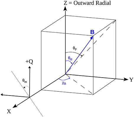
Figure 1. Observing geometry for a magnetic field located in the plane of the sky (corresponding to the ZY plane). The +Z direction indicates the local outward radial direction so moving around the solar limb corresponds to a rotation about the X axis which is taken to coincide with the line of sight. The projected angle of magnetic field on the plane sky θ_P is measured clockwise, while the angle of polarization θ_m is measured counter-clockwise adhering to the common polarimetric convention. The reference direction for the polarization measurement is oriented along the outward radial direction.

The dual-line vector magnetometry technique we propose here relies on simultaneous observations of both permitted and forbidden coronal lines. Near-IR observable coronal lines such as SiX1430, FeXIII 1.0747 μm (hereafter FeXIII1075) and HeI1083 have good polarized atomic modeling available (e.g., House, 1974; Sahal-Brechot, 1977; Casini and Judge, 1999; Asensio Ramos et al., 2008). The critical field strength B_H for the HeI1083 transition is 0.77G (Bommier et al., 1981) while the forbidden lines have critical field strengths in the 10⁻⁵G range (House, 1974). The two forbidden lines are firmly in the saturated Hanle regime, while the permitted HeI line maintains Hanle sensitivity up to ~8G. In their analysis, Bommier et al. (1981) found the unsaturated Hanle magnetic sensitivity of the HeI1083 line to be significant between 0.1B_H < B < 10B_H.

The only known visible or IR coronal permitted line is HeI1083. Using current observatories like SOLARC, it is possible to combine near-IR observations of HeI1083 with the FeXIII1075 or SiX1430 lines. When DKIST comes on-line, potentially longer wavelength IR spectropolarimetry in the near-thermal IR will be possible. To date, emphasis has been placed on FeXIII1075 observations for coronal spectro-polarimetry (Tomczyk et al., 2008), although observations during the total solar eclipse on March 29, 2006 (Dima et al., 2016, in preparation) show that SiX1430 emission can be significantly brighter than FeXIII1075. The experiment for that eclipse used a wide-field fiber fed spectropolarimeter. Figure 2 gives a comparative view of the line signal/noise in each of the fibers. During the same eclipse HeI1083 emission was also observed, although that spectropolarimeter did not have the sensitivity to demonstrate Hanle magnetometry. Nevertheless, these IR measurements clearly point to the importance of the SiX1430 line. Since the FeXIII and SiX ion abundances peak at different temperatures this result highlights the need to have multiple coronal lines accessible for polarimetry that sample different temperature regimes of the corona. While the analysis and examples presented below discuss the SiX1430 line, they can apply equally well to FeXIII1075 observations since the two lines have very similar polarization properties (Judge et al., 2006).

FIGURE 2

Figure 2. Spatial sampling of the corona during the March 29, 2006 total eclipse. A hexagonal array of 127 fibers sparsely sampled the coronal image plane. Each plot shows the signal/noise measured in each fiber for the lines indicated. One key result from these measurements is the large spatial extent of bright SiX1430 emission compared to FeXIII1075 emission.

3. Algorithm Description

Forbidden lines like FeXIII1075 and SiX1430 have radiative decay rates that are not so different from the electron collision rate at coronal densities. Thus, isotropic collisions can depolarize the Zeeman substate populations in the upper levels of the lines. Mixing occurs through both electron collisions and indirectly through cascades from excited higher levels that can have substantially higher downward transition rates (Sahal-Brechot, 1977; Judge et al., 2006). This collisional depolarization has a density dependence which is difficult to accurately model, but only affects the amplitude of the forbidden line polarization (Judge and Casini, 2001). Consequently, our method in its current form only employs the polarization angle in the forbidden lines which is independent of isotropic collisional effects.

Lines in the saturated Hanle regime maintain a fixed angular relationship between the linear polarization plane (characterized by the polarization angle θ_m and the projected magnetic field orientation on the plane of the sky (characterized by the projected angle θ_P) as shown in Figure 1. The magnetic field orientation angles (θ_B, χ_B) are related to the projected angle θ_P by

$\begin{array}{cc}\text{tan}{\theta }_{\text{P}}=\text{tan}{\theta }_{\text{B}}\text{sin}{\chi }_{\text{B}}& \left(2\right)\end{array}$

For magnetic dipole transitions like SiX1430 the polarization plane is parallel to the magnetic field when θ_B < θ_VV or θ_B > 180° − θ_VV and perpendicular when θ_VV < θ_B < 180°−θ_VV, where θ_VV = 54.7° is the Van Vleck angle. This effect leads to the Van Vleck ambiguity (e.g., House, 1974): one measured pair of Stokes Q, U corresponds to at least two pairs of possible magnetic field orientation angles. This ambiguity only applies to a subset of possible field inclinations: all linearly polarized emission from fields with θ_VV < θ_B < 180°−θ_VV is ambiguous with respect to a set of field inclinations outside this inclination domain.

In contrast, the HeI1083 permitted line has an upper level lifetime six orders of magnitude shorter. Collisions have a negligible effect on polarization amplitudes permitted lines at coronal densities. Thus, both the polarization angle and amplitude can be modeled without detailed knowledge of the coronal electron density. In our analysis synthetic Stokes I, Q, U profiles for the HeI1083 line are created using the Hanle and Zeeman Light (HAZEL)¹ code (Asensio Ramos et al., 2008). The HeI1083 line is a multiplet between the 2p³S and 2s3S terms of the triplet system of HeI. The upper term has three levels with J = 0, 1, 2 while the lower term has one level with J = 1 with corresponding transition wavelengths: 10829.09Å, 10830.25Å and 10830.34Å. The blue component is not polarizable in emission because the upper level with J = 0 has only one magnetic sublevel and is intrinsically unpolarizable. The final Stokes parameters are obtained from integrating the synthetic line profiles over the two red components which typically appear blended due to the small wavelength separation. For the analysis we choose to work in terms of the concepts of linear polarization angle and amplitude (degree) which are related to the line-profile integrated Stokes I, Q, U by the simple relations:

$\begin{array}{cc}\text{Polarizationamplitude}=\frac{\sqrt{{\text{Q}}^2+{\text{U}}^2}}{I}& \left(3\right)\end{array}$

$\begin{array}{cc}\text{Polarizationangle}=0.5{\tan }^{-1}\left(\frac{\text{U}}{\text{Q}}\right)& \left(4\right)\end{array}$

To ensure the polarization angle is correctly calculated an “arctan2”-type function should be applied. This function accounts for the signs of the U an Q values and correctly maps the polarization angle over the domain [−90°, 90°].

The algorithm steps for co-spatial sources in the plane of the sky proceed as follows:

1. From the measured forbidden line linear polarization angle θ_m we generate two sets of angle pairs (θ_B, χ_B) satisfying (Equation 2) with θ_P = −θ_m or θ_P = −(θ_m+90°). The two sets correspond to the situations where the plane of polarization is respectively parallel or perpendicular to the projected magnetic field direction.

2. HAZEL is used to generate two model Stokes profile grids for each set of angle pairs together with a suitably chosen value range for the magnetic field strength (0 < B < 8G). Thus, each point on the grid corresponds to one or more (B, θ_B, χ_B) magnetic fields. The two dimensional grids are expressed in terms of polarization angles and amplitudes calculated using Equations (3) and (4).

3. The measured HeI1083 polarization angle and amplitude are now compared to each of the model grids to find the magnetic field solution grid points consistent with the measurements and errors. If the measured linear polarization parameters only intersects the parallel model grid and lie outside the perpendicular model grid then the deduced magnetic field solution is not affected by the Van Vleck uncertainty. Alternatively if the measured value intersects both grids the deduced magnetic field has at least two degenerate solutions due to the Van Vleck uncertainty.

3.1. Example Application

To demonstrate the method we use as examples two magnetic fields with different (B, θ_B, χ_B) parameters that are typical of coronal fields (Table 1). The fields, named Fields I and II are influencing scattering points located in the plane of the sky at different heights, 0.26R⊙ and 0.08R⊙ respectively. We synthesize “measurements” using the assumed magnetic field parameters and height. HeI1083 measurements are calculated using the HAZEL code, while SiX1430 measurements are calculated using the FORWARD² code (Gibson et al., 2010) which generates polarized emission from a multi-level SiX atomic model (Judge and Casini, 2001). To synthesize the SiX1430 polarized emission we also assumed coronal electron densities typical of the heights at which the two fields are located: 0.2 × 10⁸cm⁻³ for Field I and 2 × 10⁸cm⁻³ for Field II. The larger exciting radiation anisotropy and lower densities found at larger heights leads to an increase in the amplitude of the SiX1430 polarization. For observations that are not photon limited this leads to improved accuracy for measurements higher above the solar limb.

TABLE 1

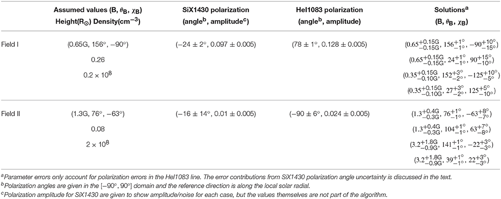
Table 1. Summary of parameters and algorithm solutions for two example magnetic field cases.

Following our algorithm two angle/amplitude grids are generated separately for Field I and II from the SiX1430 polarization angle measurement. Figures 3, 4 show the model grids generated for Field I and II respectively. By convention the polarization angle is defined over [−90°, 90°], but we redefine it for display purposes over the interval [0°, 180°] without any loss of information. This is done because the model grids shown below are easier to interpret over the modified domain. While the algorithm grid are arbitrarily dense, only some of the grid points are shown to avoid overcrowding the plot space. To visualize the variation with magnetic field strength B-isocontours are highlighted. The errors in the HeI1083 measurement are typical measurement errors of ~0.5% in the line intensity, although more accurate measurements are possible. The solution grids are not uniform so the same measurement error translates differently into inverted magnetic field errors depending on the strength of the field. Visually this is evident in the way the B-isocontours become closer together as the field strength increases. The top panel in each figure shows the full model domain while the lower panels show an enhanced view of each grid near the measured values.

FIGURE 3

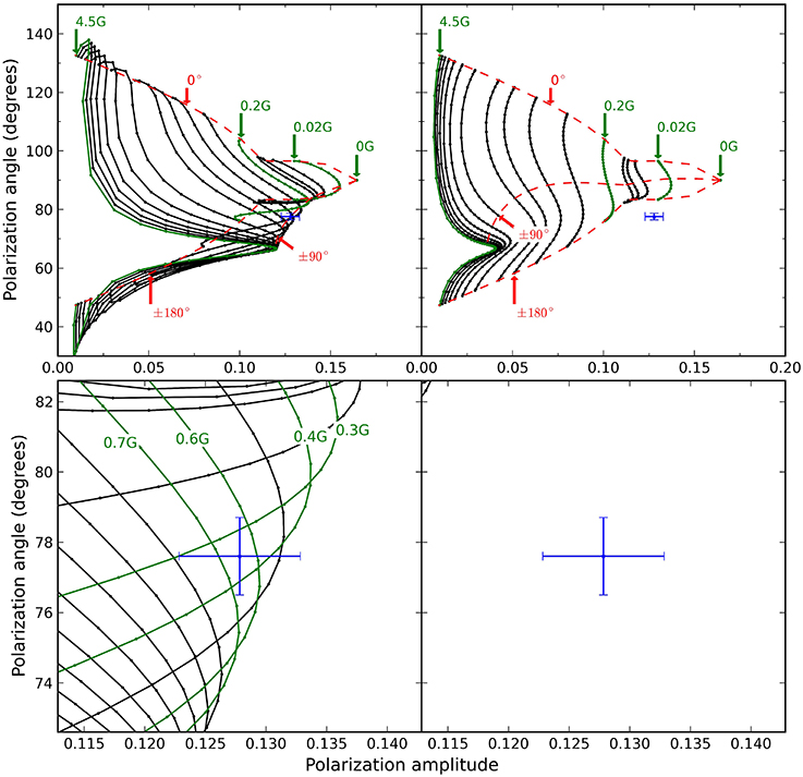
Figure 3. Field I model grids for HeI1083 linear polarization with polarization angle drawn against polarization amplitude. B-isocontours are drawn as solid black lines. The top panel shows the entire solution space with some B-isocontours highlighted and labeled in green three χ_B-isocontours drawn with red dashed.The bottom panel shows an enhanced region around the measured value for Field I with some B-isocontours highlighted in green. The B-isoncotours in the bottom panel are all separated by 0.1G. For both the top and bottom panels the left plot shows the model grids for plane of polarization parallel to the field projection, while the right plot shows the grid for the plane of polarization perpendicular to the field projection. The measured HeI1083 polarization value for Field I is drawn in blue with errors bars corresponding in size to intensity errors ~0.5%. For Field I the measurement intersects only the parallel grid. This is consistent with an inclination measurement outside the Van Vleck uncertainty region.

FIGURE 4

Figure 4. The same as Figure 3 for the Field II model grids. For the bottom panel only the B-isocontours spaced by 0.5G are drawn. For Field II the HeI1083 polarization measurement intersects both model grids which is consistent with inclination solutions inside the Van Vleck uncertainty region.

For Field I four independent solutions are obtained as shown in Table 1. The four solutions can be divided into two solution pairs with unique values of the magnetic field strength B. For each pair with a unique B there are two degenerate solutions for the angle variables θ_B and χ_B. This “classical degeneracy” is independent of the Van Vleck degeneracy and is inherent in the matter-radiation interaction problem and plane of sky scattering geometry (Bommier, 1980). The two ambiguous solutions can be obtained from each other by reflection of the B vector through the line of sight. For Field I it is evident that the measured polarization value does not intersect the solution grid for the case where the polarization plane is perpendicular to the magnetic field vector. This shows that the magnetic field is not in the Van Vleck degeneracy region.

The recovered solution space for Field II also consists of four independent solutions which can be broken down into two pairs of solutions with unique B values. Same as for Field I each pair with a unique B has two degenerate solutions for the angle variables due to the classical degeneracy. However, for Field II the origin of the different solutions for the magnetic field strength B lies in the Van Vleck degeneracy. This is seen from the fact that the measured polarization value intersects both model grids.

An important source of error in the analysis is the uncertainty in measuring the SiX1430 polarization angle. This uncertainty can be quite large as is the case for Field II due to the low radiation anisotropy and higher electron density. This uncertainty changes the parallel and perpendicular sets of (θ_B, χ_B) angles that satisfy Equation (2). The effect this uncertainty has on the model grids is shown in Figures 5, 6 for Field I and II respectively. To produce the variation shown the maximum uncertainty is added and subtracted to the measured SiX1430 polarization angle and new model grids are created using HAZEL. For Field I solutions the errors given in Table 1 are roughly one and a half time larger for all the parameters. Field II has a much larger uncertainty in measured SiX1430 polarization angle so the effect is larger but mostly concentrated in the angle determination with the variation in the angles increasing to ±25° while the magnetic field strength B uncertainty increases by one and a half times the values given in Table 1.

FIGURE 5

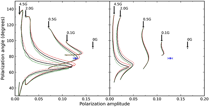
Figure 5. Shown in black are the parallel(left) and perpendicular(right) model grids for Field I as they also appear in Figure 3. The dotted lines represent added (red) and subtracted (green) uncertainties in the SiX1430 polarization angle. Only a few B-isocontours are shown and labeled to avoid overcrowding due to intersecting contour lines. The measured HeI1083 polarization parameters are shown with corresponding measurement uncertainties. Propagating the SiX1430 uncertainty requires new grids to be computed since the shapes of the grid changes as seen by the bending and crossing of model contours.

FIGURE 6

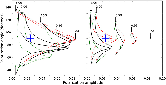
Figure 6. The same as Figure 5 but for the Field II model grids and corresponding errors. The SiX1430 linear polarization signal for Field II is weak and thus relatively uncertain for the selected realistic measurement accuracy. This uncertainty leads to the large distortions in the model grids. High accuracy forbidden line polarization directions will be required in this regime.

For these test cases we assume the line intensity measurement to be ~0.5% for both situation. Since the polarized signal for Field II is ten times weaker than the signal for Field I this translates into a significant increase in the error of the calculated magnetic field strength. However, there is nothing fundamentally limiting about the uncertainty we adopted since the source of the uncertainty is random rather than systematic. For weak polarimetric signals we can increase the integration time to improve the the uncertainty to acceptable levels for errors in the calculated parameters. To achieve the quoted 0.5% accuracy using the current spectrograph on the 0.45 m SOLARC telescope around 12 min of integration time is needed assuming a SiX1430 line brightness of $5\times 10^{-6}{\text{B}}_{\odot }$ and a spatial resolution element 7″ in diameter. The larger 4 m telescope DKIST will have improved light collecting power as well as improved signal throughput. It will make this type of accuracy possible for an observation region 1″ in diameter in less than 1 s of integration time.

4. Discussion and Conclusions

The method proposed provides important constraints on the coronal magnetic field and shows promise as a detailed magnetic field diagnostic, since it drastically constrains the coronal source region local magnetic field to four independent solutions using potentially high signal-to-noise IR linear polarization measurements. This is achieved without knowledge of polarization amplitudes for the forbidden lines that depends on the coronal electron density. It is interesting to note that the method obtains four degenerate solutions for magnetic fields located inside or outside the Van Vleck degeneracy region. Merenda et al. (2006) proposed a chromospheric algorithm that uses measured HeI1083 linear and circular polarization to determine the vector magnetic field for prominences located in the POS. Their method recovered two degenerate solutions for a magnetic field outside the Van Vleck region and four degenerate solutions for a field inside the Van Vleck region. However, all the examples analyzed by them were for field strengths in excess of 10G, which means the HeI1083 emission is in the saturated Hanle regime. From our solutions for Field I we conclude that the extra degeneracy (not related to the classical degeneracy) that appears even for fields outside the Van Vleck regions is due to the unsaturated Hanle effect. Independent knowledge of the electron density (or the forbidden line polarization amplitude) can reduce the degeneracy outside the Van Vleck region from four to two and uniquely recover the magnetic field strength B. For future work we are testing how accurate the density estimate needs to be in order to reliably distinguish between the degenerate solutions. It may be possible to exclude one pair of solutions even with an average electron model consistent with coronal white light observations.

In principle, the information on the electron density is contained in the polarization amplitude of the forbidden line which we excluded from the present algorithm. If it is possible to distinguish between the two solution pairs, we can then recover information about the electron density from the measured polarization amplitude.

Resolving the final ambiguity from the radiation field geometry requires more information. One solution to this problem is through forward modeling, using 3D coronal MHD models, perhaps constrained by photospheric magnetic field measurements. It is noticeable that these degenerate solutions have complementary values for the inclination angle, so constraints just from the photospheric magnetic polarity changes may provide the key to breaking this degeneracy. Note that similar degeneracies are encountered when measuring vector magnetic fields near the photosphere. Leka et al. (2009) summarizes the types of algorithms used to break the ambiguities in photospheric vector magnetograms. Another possibility involves using tomographic inferences from observing the same region over a few days of solar rotation. Bommier et al. (1981) successfully distinguished between ambigous solutions by observing a prominence as it rotates through the plane of the sky.

While detections of coronal HeI1083 emission shows strong correlation with streamers (Moise et al., 2010) more polarimetric observations of this line are needed to determine the exact geometry and line formation mechanisms of the emitting region. One of our principal assumptions is that the HeI1083 and forbidden line emission is co-spatial but a relaxed version of this assumption is that the emitters experience the same magnetic field. Since the magnetic field expands to fill the coronal volume it is not unreasonable to assume that some large volumes of the corona will experience the same magnetic field. However, obtaining a better understanding and characterization of the HeI1083 coronal signal in the context of simultaneous forbidden line emission measurements will provide more information toward understanding the validity of this assumption. Currently we are pursuing a dedicated campaign to obtain co-spatial and quasi-simultaneous spectropolarimetric observations of the FeXIII1075, SiX1430 and HeI1083 lines in the solar corona using the SOLARC telescope on Haleakala. These observations will form the data set needed to test the proposed method.

Author Contributions

The bulk of the effort in testing and implementing this algorithm has been done by GD in the course of developing his PhD thesis. JK conceived and advised the primary concept. SB provided support in the Hanle effect theory. SB and JK developed the funding and work plan and contributed ideas and material to the manuscript.

Funding

We gratefully acknowledge support from the NSF through grant number ATM-1358270.

Conflict of Interest Statement

The authors declare that the research was conducted in the absence of any commercial or financial relationships that could be construed as a potential conflict of interest.

The reviewer RC declared a past co-authorship with one of the authors JK to the handling Editor, who ensured that the process met the standards of a fair and objective review.

Acknowledgments

We are grateful to Tom Schad for useful clarifying discussion on the HeI spectropolarimetry. SB thanks Predictive Science Inc. and IfA, University of Hawaii for the opportunity to carry out this project as a visiting scientist. The algorithm has benefited from discussion at NSF SHINE program meetings and at the International Space Science Institute (ISSI) International Team Coronal Magnetism meetings in 2013 and 2014.

Footnotes

1. ^http://www.iac.es/proyecto/magnetism/pages/codes/hazel.php

2. ^http://www.hao.ucar.edu/FORWARD/

References

Arnaud, J., and Newkirk, G. Jr. (1987). Mean properties of the polarization of the Fe XIII 10747 A coronal emission line. Astron. Astrophys. 178, 263–268.

Google Scholar

Asensio Ramos, A., Trujillo Bueno, J., and Landi Degl'Innocenti, E. (2008). Advanced forward modeling and inversion of stokes profiles resulting from the joint action of the Hanle and Zeeman effects. Astrophys. J. 683, 542–565. doi: 10.1086/589433

CrossRef Full Text | Google Scholar

Bommier, V. (1980). Quantum theory of the Hanle effect. II - Effect of level-crossings and anti-level-crossings on the polarization of the D3 helium line of solar prominences. Astron. Astrophys. 87, 109–120.

Google Scholar

Bommier, V., Sahal-Brechot, S., and Leroy, J. L. (1981). Determination of the complete vector magnetic field in solar prominences, using the Hanle effect. Astron. Astrophys. 100, 231–240.

Google Scholar

Casini, R., and Judge, P. G. (1999). Spectral lines for polarization measurements of the coronal magnetic field. II. Consistent treatment of the stokes vector for magnetic-dipole transitions. Astrophys. J. 522, 524–539. doi: 10.1086/307629

CrossRef Full Text | Google Scholar

Gibson, S. E., Kucera, T. A., Rastawicki, D., Dove, J., de Toma, G., Hao, J., et al. (2010). Three-dimensional morphology of a coronal prominence cavity. Astrophys. J. 724, 1133–1146. doi: 10.1088/0004-637X/724/2/1133

CrossRef Full Text | Google Scholar

House, L. L. (1974). The theory of the polarization of coronal forbidden lines. Pub. Astron. Soc. Pacific 86, 490. doi: 10.1086/129637

CrossRef Full Text | Google Scholar

Ishikawa, R., Bando, T., Fujimura, D., Hara, H., Kano, R., Kobiki, T., et al. (2011). “A sounding rocket experiment for spectropolarimetric observations with the Ly line at 121.6 nm (CLASP),” in Solar Polarization 6, Vol. 437 of Astronomical Society of the Pacific Conference Series, eds J. R. Kuhn, D. M. Harrington, H. Lin, S. V. Berdyugina, J. Trujillo-Bueno, and S. L. Keil (San Francisco, CA: Astronomical Society of the Pacific), 287.

Judge, P. G. (1998). Spectral lines for polarization measurements of the coronal magnetic field. I. Theoretical intensities. Astrophys. J. 500, 1009–1022. doi: 10.1086/305775

CrossRef Full Text | Google Scholar

Judge, P. G., and Casini, R. (2001). “A synthesis code for forbidden coronal lines,” in Advanced Solar Polarimetry – Theory, Observation, and Instrumentation, Vol. 236 of Astronomical Society of the Pacific Conference Series, ed M. Sigwarth (San Francisco, CA: Astronomical Society of the Pacific), 503.

Judge, P. G., Low, B. C., and Casini, R. (2006). Spectral lines for polarization measurements of the coronal magnetic field. IV. Stokes signals in current-carrying fields. Astrophys. J. 651, 1229–1237. doi: 10.1086/507982

CrossRef Full Text | Google Scholar

Kuhn, J. R. (1995). “Infrared coronal magnetic field measurements,” in Infrared Tools for Solar Astrophysics: What's Next?, eds J. R. Kuhn and M. J. Penn (Singapore: World Scientific), 89–94.

Google Scholar

Kuhn, J. R., Arnaud, J., Jaeggli, S., Lin, H., and Moise, E. (2007). Detection of an extended near-sun neutral helium cloud from ground-based infrared coronagraph spectropolarimetry. Astrophys. J. 667, L203–L205. doi: 10.1086/522370

CrossRef Full Text | Google Scholar

Kuhn, J. R., Coulter, R., Lin, H., and Mickey, D. L. (2003). “The SOLARC off-axis coronagraph,” in Innovative Telescopes and Instrumentation for Solar Astrophysics, Vol. 4853 of Society of Photo-Optical Instrumentation Engineers (SPIE) Conference Series, eds S. L. Keil and S. V. Avakyan (Bellingham, WA), 318–326.

PubMed Abstract

Kuhn, J. R., Penn, M. J., and Mann, I. (1996). The near-infrared coronal spectrum. Astrophys. J. 456:L67. doi: 10.1086/309864

CrossRef Full Text | Google Scholar

Leka, K. D., Barnes, G., Crouch, A. D., Metcalf, T. R., Gary, G. A., Jing, J., et al. (2009). Resolving the 180° ambiguity in solar vector magnetic field data: evaluating the effects of noise, spatial resolution, and method assumptions. Sol. Phys. 260, 83–108. doi: 10.1007/s11207-009-9440-8

CrossRef Full Text | Google Scholar

Lin, H., Kuhn, J. R., and Coulter, R. (2004). Coronal magnetic field measurements. Astrophys. J. 613, L177–L180. doi: 10.1086/425217

CrossRef Full Text | Google Scholar

Lin, H., Penn, M. J., and Tomczyk, S. (2000). A new precise measurement of the coronal magnetic field strength. Astrophys. J. 541, L83–L86. doi: 10.1086/312900

CrossRef Full Text | Google Scholar

López Ariste, A., and Casini, R. (2003). Improved estimate of the magnetic field in a prominence. Astrophys. J. 582, L51–L54. doi: 10.1086/367600

CrossRef Full Text | Google Scholar

Merenda, L., Trujillo Bueno, J., Landi Degl'Innocenti, E., and Collados, M. (2006). Determination of the magnetic field vector via the Hanle and Zeeman effects in the He I λ10830 multiplet: evidence for nearly vertical magnetic fields in a polar crown prominence. Astrophys. J. 642, 554–561. doi: 10.1086/501038

CrossRef Full Text | Google Scholar

Moise, E., Raymond, J., and Kuhn, J. R. (2010). Properties of the diffuse neutral helium in the inner heliosphere. Astrophys. J. 722, 1411–1415. doi: 10.1088/0004-637X/722/2/1411

CrossRef Full Text | Google Scholar

Penn, M. J. (2014). Infrared Solar Physics. Living Rev. Solar Phys. 11:2. doi: 10.12942/lrsp-2014-2

CrossRef Full Text | Google Scholar

Sahal-Brechot, S. (1977). Calculation of the polarization degree of the infrared lines of Fe XIII of the solar corona. Astrophys. J. 213, 887–899. doi: 10.1086/155221

CrossRef Full Text | Google Scholar

Tomczyk, S., Card, G. L., Darnell, T., Elmore, D. F., Lull, R., Nelson, P. G., et al. (2008). An instrument to measure coronal emission line polarization. Sol. Phys. 247, 411–428. doi: 10.1007/s11207-007-9103-6

CrossRef Full Text | Google Scholar