Lifecycle of a Large-Scale Polar Coronal Pseudostreamer/Cavity System

1. Introduction

Streamers are large, quiescent structures in the corona which lie at and under the interface of open magnetic field domains. Streamers generally fall into two categories: “helmet” streamers and pseudostreamers, which are topologically distinct (Wang et al., 2007). Helmet, or bipolar, streamers separate regions of open opposite magnetic polarity, while pseudostreamers, also called unipolar streamers, separate open magnetic domains of the same polarity. The fundamental difference between the two types of streamers is their magnetic topology (Wang et al., 2007; Rachmeler et al., 2014). While this topological difference is well understood, it is not clear if they share similar plasma properties.

The magnetic field configurations of unipolar and bipolar streamers have been shown to have a significant role in the dynamics of the solar wind, especially in the slow component. Moreover, it has been shown that streamers and pseudostreamers are closely related to Coronal Mass Ejections (CMEs), huge releases of coronal material and energies into the interplanetary space (Howard et al., 1985; Eselevich and Tong, 1997; Zhao and Webb, 2003; Wang, 2015). They are also important tracers of the magnetic field in the heliosphere; the heliospheric current sheet extends from the top of a helmet streamer (see e.g., Borrini et al., 1981).

Streamers were first described in details in solar data much earlier than pseudostreamers (Sturrock and Smith, 1968). To date, pseudostreamer research mainly focused on their magnetic configurations and their role in both solar wind and space weather, while their thermal and density properties are poorly known. Borovsky and Denton (2013) showed that magnetic storms driven by pseudostreamers have systematically different phenomenologies than those driven from streamers. Zhao et al. (2013) proposed that pseudostreamers are associated with extreme-proton-flux slow solar wind measured by the Ulysses mission. Lynch and Edmondson (2013) showed that the pseudostreamer magnetic configuration is favorable for the breakout CME initiation mechanism. However, there are only a few studies about their thermodynamic properties (Abbo et al., 2015).

Both streamers and pseudostreamers can also contain coronal cavities, tunnel-like areas of rarefied density, which possess an elliptical cross-section (Gibson and Fan, 2006). A number of multi-wavelength studies demonstrated that cavities are depleted in density, with a typical depletion of about 30% relative to the surrounding streamers (see e.g., Marqué, 2004; Schmit and Gibson, 2011). Studies have shown that both the cavity and the streamer have temperatures in the range of 1.4–1.7 MK, though there is evidence of internal temperature variation and a hot core near the center of the cavity (Gibson et al., 2010; Schmit and Gibson, 2011; Kucera et al., 2012; Reeves et al., 2012). However, there is still no clear evidence of whether or not the cavities are typically hotter than the surrounding pseudostreamer/streamer.

Coronal cavities, often characterized by their croissant-like morphology in three dimensions (3D), provide important information about the magnetic structures that support prominences. The magnetic energy is stored through the non-potentiality of the twisted or sheared magnetic field associated with the prominences. This energy is ultimately released through CMEs. To be able to forecast these energetic releases of material and prevent potential terrestrial consequences, the understanding of its three dimensional morphology and its magnetic field is essential. The prominences embedded in the cavity only trace a small part of the magnetic field, whereas the much larger cavity provides more information about the magnetic field morphology. As a result, a clear understanding of the coronal volume of the cavity significantly advances our understanding of both the pre-eruption equilibrium and the triggers of such eruptions.

Determining both morphological and thermodynamical coronal structures is difficult due to the optically thin nature of the plasma. UV and visible observations are subject to integration along the line-of-sight (LOS). This effect can strongly complicate both the derivation and the interpretation of important physical quantities. The background and foreground emission can easily overwhelm the signal of interest, leading to a loss of information about the 3D geometry.

One way to deduce the 3D structure is with solar rotational tomography (SRT). In general terms, tomography is a technique used to determine the 3D structure of an object. Many different areas of science—such as medicine, geophysics, and astrophysics—use this class of technique. For the particular case of SRT, the plasma emissivity is estimated from EUV/white light images taken from different viewpoints, mathematically corresponding to the inversion of the LOS-integration. Physical properties can be then derived from these multi-wavelength emissivities. Tomography is a highly under-determined problem (Aschwanden, 2011), and the intrinsic difficulties of non-robustness and non-uniqueness of the solution have to be overcome. SRT in particular is further complicated by the lack of simultaneous viewpoints, which is limited by the number and location of available spacecraft. Multi-spacecraft observations in the optimal position when possible, coupling with the natural solar rotation provides the necessary multiple points of view. Tomographic inversion generally assumes that the structure to be inverted is not time-varying, complicating the inversion process. The reconstruction is further complicated by the fact that the Sun rotates differentially and coronal features can change during a rotation. As a result, the inverse-problem is further ill-posed. In practice, the inversion codes assume rigid rotation and non-evolving structures, although some authors developed techniques to overcome the time variability (e.g., Barbey et al., 2008; Butala et al., 2010; Barbey et al., 2013). In this work, we propose a simple alternative to these challenges using a technique of sliding time-windows.

Due to rapid progress in inversion algorithms, faster computation facilities, and the availability of new data, SRT has been recently used for the study of a variety of coronal structures observed in EUV. Nuevo et al. (2015) used a technique similar to the one used in this work in order to determine the 3D thermal structure of the corona. Their measurements revealed the omnipresence of bi-modal DEM within the quiet corona, with clearly distinct cool and hot components. Huang et al. (2012) and Nuevo et al. (2013) used a combination of tomography and magnetic field extrapolation (the Michigan Loop Diagnostic Technique - MLDT) to determine the temperature along quiet-Sun coronal loops. Morphological properties of polar plumes have also been investigated by de Patoul et al. (2013), and using Hough-wavelet transform and filtered-back projection tomography, the authors determined the plumes temporal variation and cross-sectional shape. Vásquez et al. (2009) presented tomographic measurements of polar-crown cavities using the DEMT method of (Frazin et al., 2005b). They found density-depleted cavities (about one-third) and broader thermal distribution shifted toward higher temperatures, relative to the surroundings streamers. For an exhaustive review about general solar tomography, the reader is referred to Aschwanden (2011).

In this paper, we report the observation of an exceptional large-scale coronal pseudostreamer/cavity system in the southern polar region of the solar corona, which was visible for approximately a year starting in February 2014. It is unusual to see such a large closed-field structure embedded within the usually open polar region. We tracked the formation, evolution and disappearance of the pseudostreamer/cavity system using SRT. To our knowledge this is the first time that SRT has been applied specifically to a pseudostreamer system. We tracked the 3D plasma parameters and their evolution over the whole life-cycle of the pseudostreamer, using a combination of both tomography and DEM inversions. The technique of SRT is complementary to coronal magnetometry, as different domains of plasma parameters correlate with the magnetic structure. Used together, they can provide a powerful diagnostic of not only the magnetic structure of the corona, but also the feedback between the plasma and the field.

2. Methods : Measuring the 3D Thermal Structure

To derive the plasma properties of the structure and evolution thereof, we couple SRT and differential emission (DEM) analysis. We first use SRT to determine the three-dimensional emission of the plasma in multiple EUV wavelength bands. For each location in space, we then use the emissivity in a differential emission analysis (Pottasch, 1963) which calculates the plasma density and temperature at that location.

2.1. Solar Rotational Tomography

The first step in our analysis is to estimate the three-dimensional distribution of the coronal plasma emissivity. We used the SRT software TomograPy, described in Barbey et al. (2013), an open-source program freely available in the Python Package Index¹. The software performs fast tomographic inversions using one of several parallelized-projection algorithms. Various types of solar image data can be used as input including multiple UV wavelengths and white-light observations.

In the case of optically thin plasma, the intensity I_b, produced by collisional emission lines and continua in a given UV or EUV waveband b, integrated along the LOS l, can be expressed as

$\begin{array}{cc}{I}_b={\displaystyle {\int }_{-\infty }^{\infty }{R}_b(n_e,T_e)n_e^{2}dl}& \left(1\right)\end{array}$

where R_b is the response function to a unit volume of plasma of electron temperature T_e and density n_e of the instrument. This temperature response function takes into account the intensity produced by each emission line, the contribution of the continuum, and the spectral sensitivity of the instrument band b. The function R_b accounts for all of the physics of the radiation emission process (see e.g., Mason and Fossi, 1994). Given a simple case where the input is EUV images from a single spacecraft, and assuming that the Sun does not change during the observation window, SRT inverts the integration along the LOS and solves for

$\begin{array}{ll}{e}_{b,i}=R_b(n_e,T_e)n_e^2,& (2)\end{array}$

the local emissivity of the coronal plasma. In this case, we can easily discretize Equation (2), assuming that the reconstructed object-map is a cubic regular grid centered on the Sun

$\begin{array}{ll}{I}_j={\displaystyle \sum _i}{P}_{i,j}{e}_i+n_j& (3)\end{array}$

where I_j is the intensity in the image pixel j, e_i is the local emissivity in the voxel number i along the LOS, P_{i, j} is the length of the portion of the LOS j passing through the voxel i, i.e., the volume element of the 3D reconstruction grid, and n_j is the noise associated with the image pixel j. Equation (3) can then be rewritten in matrix notation

$\begin{array}{ll}I=\mathrm{Pe}+n& (4)\end{array}$

where I contains all the pixels of every image of size N and e the reconstruction cube of size M. The projection matrix P, called the projector in TomograPy, takes into account the position and the orientation of the spacecraft for each pixel of each image used in the reconstruction. To compute the exact path of each LOS through the various voxels, the software uses a parallelized implementation of the Siddon algorithm (Siddon, 1985) in C. Designed for Cartesian grid, this algorithm computes the projection or back-projection operations very quickly, and the huge projection matrix of size M × N does not need to be stored in memory.

The tomographic inversion process is likely to be under-determined and highly ill-conditioned, and thus the direct inversion of Equation (4) is not feasible. The TomograPy software uses Baye's formalism to solve this tomographic linear inverse problem, fully equivalent to classical regularization methods (see e.g., Frazin et al., 2005b; Barbey et al., 2008, 2013). In this approach, we define a prior model which encompasses all the a priori available information on the unknown true solution, e. Usually, the prior is chosen to be the finite-difference operator, which favors a smoother solution, and thus suppresses noise. Using the following minimization process, we calculate the our estimated local emissivity cube, $\widehat{e}$:

$\begin{array}{ll}\widehat{e}={\displaystyle \underset{e}{\text{arg}\text{min }}}\left\{\left|\right|y-Pe|{|}^2+\lambda |\left|\mathrm{DR}e\right|{|}^2\right\}& (5)\end{array}$

where the first term relies on a simple least-square inversion. The a priori information is given by the second term, where D is the finite-difference operator, λ ≥ 0 is a free parameter controlling the smoothness, and R² is a diagonal smoothing prior, increasing with height. Solar image data becomes noisier with height, as the true signal strength drops off. The R² serves to suppress the influence of this noise in the tomographic solution. Additionally, as other SRT methods use spherical grids, R² improves the similarity of solutions between the cartesian and spherical grid implementations. This is because the voxel size grows with height in spherical grids, increasing the signal-to-noise ratio there.

Our tomographic reconstruction technique is closely related to the method of Frazin et al. (2005b), except for some technical aspects. The main differences are their use of a spherical grid and their imposition of positive-only solutions; we use a Cartesian grid and allow negative values of the emissivity. Negative values in tomographic reconstructions are obviously not physical, but their presence reveals temporal evolution in the solution. Static tomography assumes that the emissivity in each voxel is constant over time. But when temporal evolution is present, as it is in the Sun on rotational timescales, this assumption is not strictly valid, and our algorithm compensates for this behavior by introducing negative values, which allow us to identify areas that are subject to evolution.

2.2. Coupling DEM Analysis and Tomography

While tomography is used to alleviate the ambiguity imposed by LOS integration through an optically thin plasma, the DEM analysis quantifies the temperature distribution of the plasma along the LOS, without regard for its morphological properties. Introduced by Pottasch (1963) for elemental abundance measurements, the DEM is now widely used in the solar community, for all types of coronal structures. The DEM provides a measure of the amount of emitting material along the LOS as a function of the electron temperature T_e. Recasting Equation (1) as a function of the temperature, the intensity observed in an UV band is given by

$\begin{array}{cc}{I}_b={\displaystyle {\int }_0^{\infty }{R}_b(n_e,T_e)\xi (T_e)d\log T_e.}& \left(6\right)\end{array}$

The DEM ξ is defined as

$\begin{array}{ll}\xi (T_e)=\overline{n_e^2}(T_e)dp∕dlog{T}_e\left[{\text{m}}^{-5}.{\text{K}}^{-1}\right]& (7)\end{array}$

where $\overline{n_e^2}$ is the square electron density averaged over the portions dp of the LOS at temperature T_e (see Craig and Brown, 1976, for details). Nevertheless, reliably inferring the DEM from observations is a genuine challenge, due to the inverse nature of the problem. The fundamental limitations of DEM inversion have been discussed in e.g., Jefferies et al. (1972); Craig and Brown (1976); Brown et al. (1991); Judge et al. (1997) and more recently by Testa et al. (2012); Guennou et al. (2012a,b), including issues due to noise in the input measurements, systematic uncertainties, the width and the shape of the temperature response functions, and the associated consequences of multiple solutions.

These two techniques are linear inverse problems and the coupling of the both leads to the estimation of the three-dimensional distribution in temperature and density of the coronal plasma. Frazin et al. (2005b, 2009) were the first to propose such a combination of these two techniques, in a procedure called Differential Emission Measure Tomography (DEMT), demonstrating the ability of such a diagnostic to distinguish plasma of different temperatures from multi-waveband EUV observations. Tomography mitigates the integration along the LOS, but the temperature is still unlikely to be constant within a given voxel volume, as the typical voxel volume is ~8000 km³. We can thus define a local DEM by recasting Equation (2) as

$\begin{array}{cc}{e}_{b,i}={\displaystyle {\int }_0^{\infty }{R}_b(T_e,n_e){\xi }_{loc,i}(T_e)d\log T_e,}& \left(8\right)\end{array}$

with ξ_loc the local DEM of the ith voxel, defined over the volume voxel V_i rather than a portion of the LOS as

$\begin{array}{ll}{\xi }_{loc,i}=n_e^2(T_e)d{V}_i∕dlog{T}_e\left[{\text{m}}^{-3}.{\text{K}}^{-1}\right]& (9)\end{array}$

assuming that the density n_e is constant over the voxel volume (see Brown et al., 1991, for a rigorous definition of the volumetric DEM). Analogous to the classical DEM, the local DEM describes the temperature distribution of the plasma within the voxel, therefore at a smaller scale than the grid itself. Because the integration volume is significantly smaller for the local DEM than for the classical DEM formalism, the temperature variation within the voxel should be substantially reduced.

Once we have estimated the local plasma emissivity cubes, ${\widehat{e}}_b$, estimated independently for each waveband by solving Equation (4), we are then able to determine the local DEM for each voxel. A variety of classical DEM algorithms have been proposed (e.g., Kashyap and Drake, 1998; Hannah and Kontar, 2012; Cheung et al., 2015, and references therein), easily adjustable to plasma emissivity rather than intensity. However, we only have at maximum the six coronal channels available in this work, and therefore the complexity of the reconstructed local DEMs is limited. We chose to limit the possible local DEM solutions to Gaussian distributions defined by three parameters, central temperature T_c, amplitude n_e and width σ, as

$\begin{array}{l}\begin{array}{c}\hfill {\xi }_{loc,i}=n_e^2(T_e){N}(log{T}_e-log{T}_c)\end{array}\\ \text{with}{N}(\text{x})=\frac{1}{\sigma \sqrt{2\pi }}exp\left(-\frac{x^2}{2{\sigma }^2}\right).& (10)\end{array}$

There is no physical reason the temperature distributions within a voxel should follow a Gaussian. Nonetheless, this formalism is able to describe a great variety of plasma conditions, and is simple enough to allow easy computation of the local DEMs for a large number of voxels. Additionally, Gaussian local DEM inversions have been fully analyzed and calibrated by Guennou et al. (2012a,b), allowing us to identify possible secondary solutions.

We determine the local DEM ξ_{loc, i} for each voxel, using a simple least-square criterion

$\begin{array}{cc}{\chi }^2=\min \left[{\displaystyle \sum _{b=1}^{N_b}{\left(\frac{e_{b,i}^{\text{tomo}}-e_b^{\text{synth}}(T_c,n_e,\sigma )}{{\sigma }_{b,u}^2}\right)}^2}\right],& \left(11\right)\end{array}$

where N_b denotes the number of wavebands (6 for AIA), and ${\sigma }_{b,u}^2$ are the uncertainties related to calibration, atomic physics, and instrumental noise, estimated to be 35%, according to Guennou et al. (2012a). For each waveband the synthetic emissivities $e_b^{\text{synth}}$ are calculated through

$\begin{array}{cc}\begin{array}{l}{e}_b^{\text{synth}}(T_c,n_e,\sigma )=n_e^2{\displaystyle {\int }_0^{\infty }{R}_b(T_e,n_e){N}(\log T_e-\log T_c)d\log T_e}\\ =n_e^2(R_b\ast {N})(T_c,\sigma ).\end{array}& \left(12\right)\end{array}$

We note that the synthetic emissivities are equal to the convolution product of the temperature response function by the Gaussian local DEM. They correspond to the expected emissivity values for all possible combinations of the three local DEM parameters n_e, T_c, and σ. The response temperature R_b(T_e) of the six AIA coronal bands have been computed using version 7.1 of the CHIANTI atomic database (Dere et al., 1997; Landi et al., 2013). The temperature varies from log T_e = 5 to log T_e = 7 in steps of 0.0025 log T_e, whereas the density covers the range from 10⁷ to 10¹⁰ cm⁻³ in steps of 0.01log n_e. The local DEM width varies linearly in 80 steps from σ = 0 to σ = 0.8 log T_e. This choice of sampling leads to pre-computed emissivity cubes with ~2 × 10⁷ elements for each AIA band, which are easily manageable data cubes.

The final result of the our analysis gives us the emissivity in each bandpass for each voxel location, as well as the local DEM obtained from these emissivities. From the local DEM analysis, we extract the temperature (i.e., the central temperature of the Gaussian local DEM), the density, and the Gaussian local DEM width, which corresponds the thermal width of the plasma, for each voxel. Thus, in conjunction with the time analysis described in the next section, we can track the evolution of both morphological and thermal properties of our observed large-scale polar pseudostreamer.

2.3. Tracking the Time Evolution

A common source of error in SRT is the dynamic nature of the corona during rotational timescales. Even using multiple simultaneous points of view when possible, we still need a few days of data acquisition to generate a tomographic map. Auchère et al. (2012) reduced this to 5 days of data using three separate spacecrafts: STEREO/EUVIA, STEREO/EUVIB (Wuelser et al., 2004), and PROBA2/SWAP (PRoject for Onboard Autonomy 2/Sun Watcher using Active Pixel system detector and image processing Seaton et al., 2013). Some authors have developed methods attempting to overcome this issue, which take into account the temporal variation of coronal structures. Barbey et al. (2008) developed a 3D model for plumes, in which plumes are considered to be static objects—but objects whose intensity is allowed to vary. This method is especially tailored for plumes as they can sporadically appear and disappear at the same place. Barbey et al. (2008)'s results show a great improvement of the quality of plume reconstructions. Smooth temporal SRT, providing global 4D reconstructed cubes, have been developed by Frazin et al. (2005a) and Butala et al. (2010) using Kalman filtering, and later by Barbey et al. (2013), showing that allowing temporal variation leads to qualitatively better reconstructions.

In this work, we chose to adopt a different approach to combat this issue. Instead of seeking to model the temporal evolution of the whole corona, and thus increasing the degree of under-determination of the inverse problem, we instead search for the stable structures within our reconstructions. To achieve this, we use sliding-windows in time to reconstruct the corona. We compute a reconstruction of the corona using a 17 day window, which is then shifted by 1 day at a time for a total time coverage of approximately a year. If a structure is completely stable over a long period of time, it will be detected at the same location in successive reconstructions. On the other hand, the artifacts created by temporal evolution or other projection effects (see Sections 5 and 4 for more details) will change significantly between successive reconstructions. In this way, we can differentiate between static structures and artifacts and ensure that certain observed structures are real.

The differential rotation of the Sun is another issue of concern for coronal tomography. On the photosphere, the rotation rate varies with latitude, with faster velocities close to the equator. However, the rotation rate of the corona is still uncertain, many studies have shown that the differential rotation in the corona is weaker than on the photosphere. Altrock (2003) suggest that structures with lower temperatures rotate at a slower rate. Polar coronal holes for example, show rotation rates close to rigid body, according to the study of Wang et al. (1988). Given the difficulties and uncertainties mentioned above, we do not currently take differential rotation into account in SRT. The photospheric rotation rate close to the pole is about 10.53° per day. This is the reason why we used 17 days of data for each reconstruction, to ensure over 180° of coverage in longitude (only half a rotation is needed at the poles since the plasma is optically thin), in the extreme case that some structures could be subject to different rotation rates.

3. Observations

The large scale pseudostreamer that is the subject of this paper lasted around 1 year, beginning in February 2014. We used the SWAP 174 Å and AIA 94, 131, 171, 193, 211, 335 Å UV coronal images to follow its evolution and produce the tomographic and local DEM inversions. To observe the formation process of this long-lived pseudostreamer, the SWAP data time series begins on 2013 December 19, about 2 months before its formation. We tracked its evolution until 2015 March 31. For AIA, we used observations from 2014 January 1 until 2015 February 28. In March 2015 two gaps in the AIA data prevent us from computing accurate tomographic reconstructions: from March 1 to March 5 and from March 8 to March 14.

The SWAP data were fully calibrated using the SolarSoft IDL p2sc_prep routine which removes dark current, corrects for the flat field, deconvolves the point spread function, and corrects the image so that the Sun is round, centered, and solar north is up. To create high signal-to-noise images, 100 min of data were median-stacked to create a single frame for input into TomograPy. The processing steps and the median-stacking of the images was described in more detail by Halain et al. (2013) and Seaton et al. (2013). The median-stacking suppresses short-time-scale dynamics of the Sun, which improves the tomographic inversion accuracy. For each tomographic inversion, 17 days of data at a cadence of 100 min (totalling ~240 median-stacked frames) were used.

To examine the thermal distribution of the corona, we used AIA images from the six coronal waveband channels. For each waveband, the data were first rotated, translated, scaled and normalized, using a Python function equivalent to the SSW routine aia_prep.pro. Then, 10 images (1 frame per minute) were averaged together to create a single frame with high signal-to-noise ratio. For each tomographic inversion, 17 days of data at a cadence of 2 h (totalling ~204 averaged frames) were used.

Figure 1 depicts the evolution of the streamer over time, as shown by SWAP in the 174 Å waveband using a linear and inverted intensity scaling. The full lifecycle is shown from pre-formation to post-disappearance; the images in Figure 1 depict data from 2014, January 15, February 23, July 11, October 05, December 19, and 2015, March 17. An animation showing the entire 15 months of SWAP data is available in the online material. Additionally, Figure 2 shows the schematic view of the evolution of the streamer/pseudostreamer magnetic field configuration. The magnetic field configuration and evolution, jointly with the corresponding magnetograms, will be discussed in more details in a follow-up paper (Rachmeler et al., in preparation).

FIGURE 1

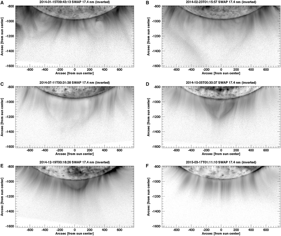
Figure 1. Evolution of the pseudostreamer observed with SWAP 174 Å waveband. Color scale is inverted, so black corresponds to the higher intensity values.

FIGURE 2

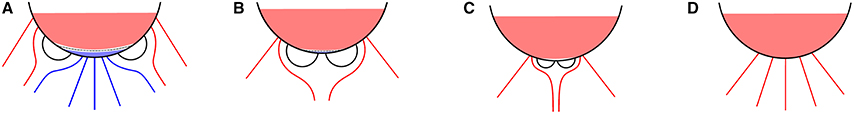
Figure 2. Schematic view of streamer to pseudostreamer transition (A,B), followed by the shrinking of the pseudostreamer (C) until its complete disappearance (D). The polarity inversion line is indicated by the dashed black line; domains of opposite polarity are denoted by the open red and blue field lines; closed lines are in black.

Before the pseudostreamer forms, a streamer encircles the entire pole, as seen in Figure 1A. The neutral line, corresponding to the filament channel, and base of the cavity (Vial and Engvold, 2015), surrounds the pole (highlighted by a dashed line in Figure 2A), and the corresponding polar-crown cavity is apparent as two cavity lobes in the plane of the sky, with suppressed EUV emission (lighter gray in the inverted SWAP images). Open field at the pole has a positive polarity, which was the dominant polarity of the previous coronal hole (blue in Figure 2), separated by the streamer from regions with negative polarity (red in Figure 2).

The polarity inversion line then drifts toward the pole, reducing the area of open field lines at the pole. By dint of this gradual displacement, the remains of the old polar coronal hole shrink until the open field disappears completely at which time the structure transitions from a 360° steamer to a topologically different pseudostreamer, as shown in Figure 2B. This transition first occurs on 2014 February 22. Subsequently a pseudostreamer can be seen at intervals during a period of about 2 month, suggesting irregular oscillations between streamer/pseudostreamer configurations. Afterwards, the pseudostreamer is definitively established, and observable until 2015 March 11. This new pseudostreamer magnetic field configuration is illustrated schematically in Figure 2B. All open field lines now have the the new (that is, negative/red) polarity, except photospheric regions south of the polarity inversion line which still have the old (positive/blue) polarity. At this point, the corona and the heliosphere have reversed their polarity, but the photospheric polar field has not. Figure 1B shows the newly formed pseudostreamer, as bright strands (i.e., darker area) above the pole, surrounding the closed loops. A cusp-shape void can be observed at the top of the pseudostreamer, likely corresponding to plasma at hotter temperature than the SWAP 174 Å waveband.

Afterwards, the polarity inversion line continues to move toward the pole, and the pseudostreamer shrinks(see Figure 2C). The gradual shrinking can be observed in Figures 1B–E, where the pseudostreamer apex decreases from about 1.6 R_⊙ (b) to about 1.1 R_⊙. The bright ray emanating from the top of the pseudostreamer corresponds to the separatrix between distinct magnetic domains (Rachmeler et al., 2014). Once the pseudostreamer and the associated polarity inversion line completely disappears, the south pole magnetic field has fully reversed.

4. Tomography : Morphological Properties

In order to further increase the signal-to-noise ratio for SWAP data, we performed the daily tomographic reconstructions using images spatially binned by a factor of 4, resulting in 256 × 256 pixel images. The reconstruction cubes are centered on the Sun with a size of 256 × 256 × 256 voxels and with a width, height, and depth of 3.5 R_⊙ each. To compute the solution, we minimize Equation (5) using a hyper-parameter, corresponding to the parameter of the prior distribution, λ = 0.45, estimated empirically by the authors using simulations, although some methods exist to evaluate it automatically (see e.g., Higdon et al., 1997; Frazin, 2000; Frazin and Janzen, 2002). For AIA data, the same parameters were used, except for the spatial binning of the images by a factor of 16 due to AIAs higher initial spatial resolution.

Figures 3, 4 show the SWAP local emissivity, in units of Digital Numbers (DN) as a function of solar radii, in selected reconstruction cubes at a constant altitude of 1.05 and 1.10 R_⊙, respectively. A gnomonic projection is used, and longitude and latitude (assuming that the origin 0° is at the equator) are reported accordingly. Negative values are highlighted in gray. Movies showing the all of the reconstruction cubes with polar views at 1.05, 1.10, and 1.15 R_⊙, and the corresponding time standard deviation maps (described in Section 5) covering the whole 15 month period are available in the electronic version of this journal.

FIGURE 3

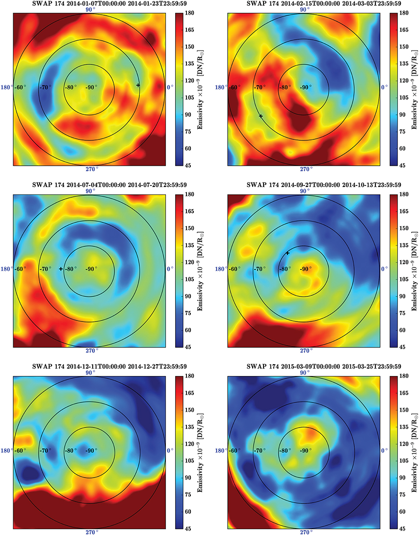
Figure 3. SWAP polar view of the south pole at 1.05 R_⊙ for select tomographic reconstructions corresponding to the images in Figure 1. The black plus represents the position of the cavity center (see text for details).

FIGURE 4

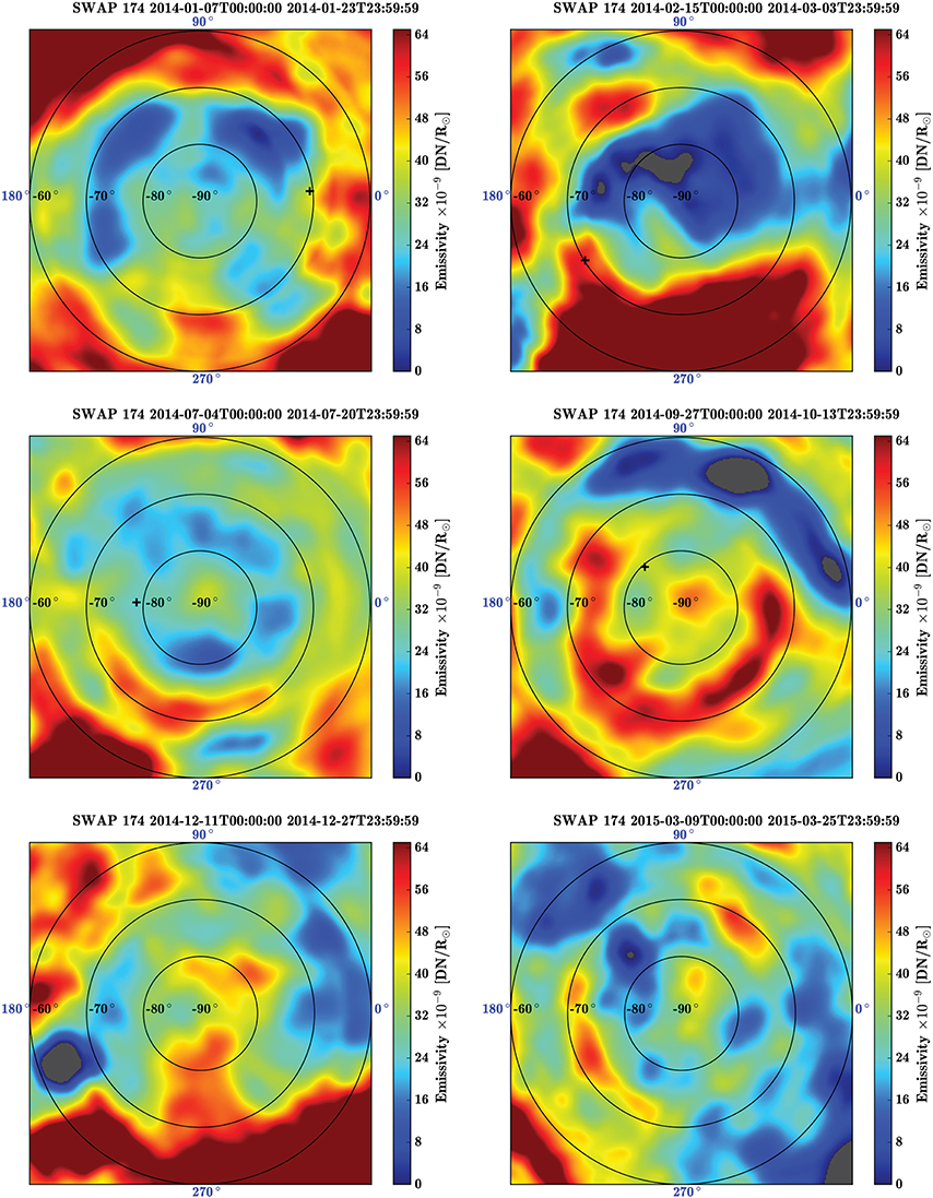
Figure 4. Same as in this Figure, but for an altitude of 1.10 R_⊙. Note that the positions of the cavity center (black plus) were measured at 1.05 R_⊙.

The reconstruction cubes in Figures 3, 4 correspond to a time window centered on the SWAP images in Figure 1. For each polar view, the black plus sign represents the position of the cavity center, measured at a constant height of 1.05 R_⊙. This was done by tracing the latitudinal emissivity profile in our data cubes for the longitude corresponding to the central meridian of the time centered image of the SWAP data used. The central position of the cavity was chosen to be the local minimum of the profile, closest to the emissivity peak associated with the pseudostreamer.

In both Figures 3, 4 (see also the movie online), a part of the projections, in the longitude area opposite to the marked cavity position, is smoother and presents lower emissivity. This artifact, which is more pronounced at higher altitudes, is due to the fact that we used 17 days of data (approximately half a solar rotation), as opposed to a full rotation. In the Siddon algorithm, the LOS are stopped once they hit the photosphere, and therefore some parts of the pole are poorly constrained in the reconstruction process. Because we used a 1 day time sliding window for our reconstructions, a low emissivity structure can be seen in the online movies, always located on the other side of the sun from the marked cavity positions. The choice of using only 17 days of data instead of a full rotation is valid as we are mainly interested in the volume above the pole that is never blocked by the solar limb, but it still results in reduced emissivity in the back side of the Sun. In order to obtain a better estimation of these locations, ~7 more days of data can be added to each reconstruction, but this would in turn exacerbate the artifacts due to temporal variations, inducing negatives values in the reconstructions. Because the reconstructions maintain a fixed central meridian, the viewing angle of the solar images rotates around the pole. Thus, the region of lower emissivity appears to rotate or swirl with time in the movies. This rotation is purely due to the low-emissivity artifact, and is not associated with solar differential rotation.

The polar views of Figures 3, 4 clearly show the three dimensional morphology of the pseudostreamer. A distinct decrease of the mean emissivity over time is clearly visible in sucessive frames of the figure, indicating that the activity at the pole slightly decreases as the pseudostreamer shrinks. At first, in January 2014 (top left), when the pseudostreamer is not formed yet, the cavity, corresponding to regions of lower emissivity (i.e., in green and blue), encircles the entire pole and is mostly circular, titled by about 7° relative to the Carrington frame, and located between −60 and −70° in latitude. The bright streamer material (in red) equatorward of the cavity also encircles the pole, and is located around −60° in latitude, although it does dip closer to −70° latitude near 90° longitude. In February (top right), once the pseudostreamer is formed, structures are more complex, as can been seen in Figure 1B and there is no longer clear circular symmetry. The pseudostreamer is visible in the half of the pole centered around the marked cavity position. The cavity—and thus the neutral line as well—is not obviously continuous, and only located between 210 and 40° longitude. Nonetheless it is still located around −60° in latitude, as it was in January. The following frame shows the well-established and stable pseudostreamer (see the online movie of SWAP data), and its shrinking can be observed in the subsequent polar projections. The pseudostreamer exhibits a clear circular symmetry, with an embedded circular cavity. In July (middle left) and October (middle right), the pseudostreamer, and thus polar crown cavity, slowly move toward the pole, with cavity positions at about −78 and −81° latitude, respectively, fully in agreement with the cavity position measured in the SWAP images (Figure 5). In December (bottom left), the suppressed emissivity region is very small and centered on the pole. Finally, in March (bottom right), the pseudostreamer has disappeared completely, and the coronal hole covers the whole pole. Some remnant structures are observable within the coronal hole, identified as bright nodules that are associated with the plumes observed in Figure 1F.

FIGURE 5

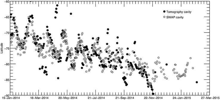
Figure 5. Cavity positions in both tomographic reconstructions (black dots) and images (gray circles), as a function of time. The periodic variations are due to the tilt of the polar crown cavity with respect to the solar rotation axis. On average, there is a very good agreement between the two measurements, demonstrating the consistency of the tomographic reconstructions.

In order to compare our long-term tomographic reconstructions with the series of 15 months of SWAP data, we compare the cavity position measured both in the cubes and in the initial data, reported in Figure 5. The position of the cavity in the tomographic reconstructions was made as described above in this section. In the images, this was done by eye, by selecting at 1.05 R_⊙ the center of the cavity (i.e., with lower intensity) in the plane of the sky on both western and eastern edge (Rachmeler et al., in preparation). Latitudinal cavity positions were then de-rotated by a quarter-rotation to be able to compare both measurements. Figure 5 shows that there is an excellent agreement between tomographic measurements (black dots) and the SWAP cavity positions (gray circles), indicating clear consistency between images and tomographic reconstructions. The periodic shape of the curves is due to an offset between the Suns rotation axis and the cavity's symmetry axes. Some tomographic measurement points in late March and early May are far away the curves. The first period occurred when the structure oscillated between a streamer and a pseudostreamer, while the second period contained many dynamic events.

The pseudostreamer is particularly steady and thus very well reconstructed from early June to mid-October, 2014. In the rest of this section, we discuss a single reconstruction using data from July 14 to 30, which we will call the July 14th reconstruction. Figure 6 shows the reconstructed polar view at 1.05 R_⊙ using the six coronal channels of AIA at 94, 131, 171, 193, 211, 335 Å (from left to right, top to bottom). Images are saturated in order to enhance the contrast between dark and bright structures, and the SWAP cavity position is also superposed as a black plus-sign on each image. The cavity is strongest in the 131 (top right), 171 (middle left), and 335 Å (bottom right) wavebands, but still visible in the other channels. In the 171 Å waveband (middle left), the cavity exhibits a quasi-circular shape, between −70 and −80° in latitude. The polar crown cavity is less visible in the 193 and 211 Å channels, corresponding to temperatures of around 1.2 × 10⁶ − 2 × 10⁷ and 2 × 10⁶ K, respectively. However, the cavity is clearly discernible in the 131 Å waveband, which is sensitive to very hot plasma temperatures around 10 − 15 MK. Note that the low signal region in the bottom left corner of each images is the artifact due to the lack of data covering that longitudinal area, as described above. The cavity is embedded in the polar crown pseudostreamer, the outer edge of which is clearly visible in each image as a bright ring just equatorward of the cavity. Using these six reconstruction cubes, we present in the next Section, 5, the corresponding DEM inversion and time analysis.

FIGURE 6

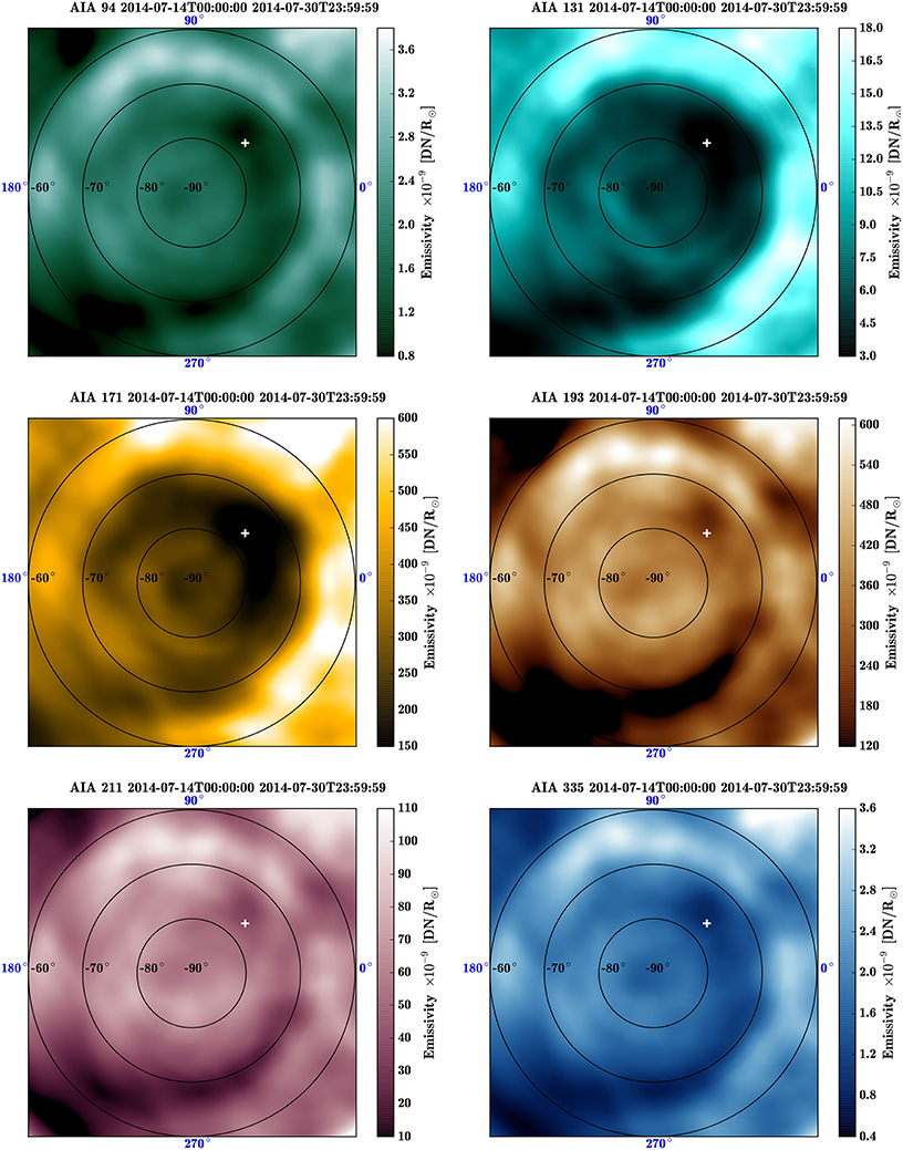
Figure 6. AIA polar view for each coronal channel (94, 131, 171, 193, 211, 335 Å, from top to bottom, left to right), at a constant altitude of 1.05 R_⊙ for an AIA data window covering July 14–30, 2014. The position of the cavity center (white plus) measured in the SWAP reconstruction (174 Å) is indicated on each figure.

5. Coupling the DEM : Thermal Properties

Following the method described in Section 2.2, we obtained the local DEM associated with each spatial location of our reconstruction cubes, for the whole period considered. Full results for the entire time interval studied here are available on the online version of this journal and are discussed in Section 5.2.

5.1. Example: The July 14th Tomographic/DEM Reconstruction

The Gaussian DEM inversion results corresponding to the AIA reconstructions presented in Figure 6 are displayed in Figures 7, 8, showing a collection of polar views at 1.05 and 1.10 R_⊙, respectively. The corresponding SWAP reconstruction is shown on the top left panel, with the cavity position marked by a black plus sign, which is also indicated on each subsequent image in the figure. The 3 Gaussian DEM parameters, i.e., the central temperature T_c, the density n_e and the thermal width σ (see Equation 10) are displayed on the top right, middle left and middle right panels, while the corresponding χ² residual (see Equation 11) is shown on the bottom left panel. Note that the low signal region in the bottom left corner of each images is the artifact due to the lack of data covering that longitudinal area, as described in Section 4.

FIGURE 7

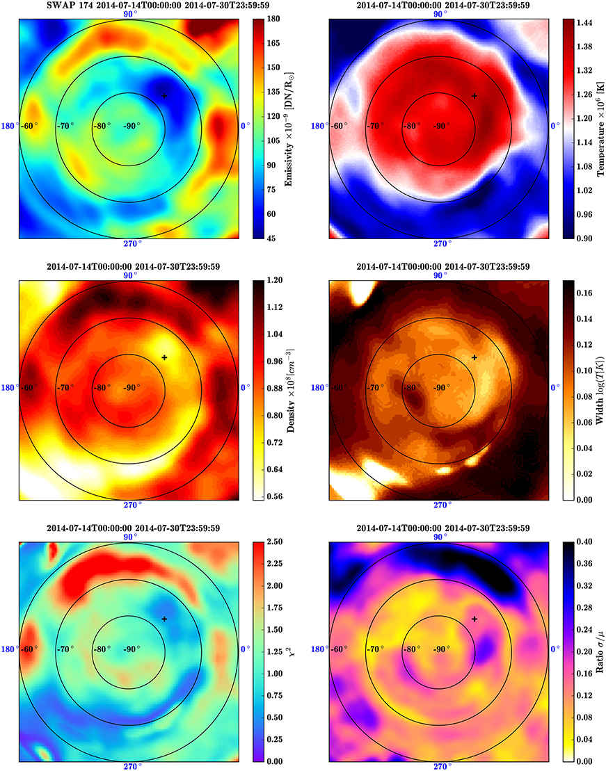
Figure 7. Example of full tomography/Gaussian DEM coupling analysis at 1.05 R_⊙ corresponding to the AIA polar view presented in Figure 6. The black plus sign is the cavity position measured in the SWAP cubes at 1.05 R_⊙. Top left: Corresponding SWAP polar view. Top right: Temperature [K], i.e., the central temperature T_c of the assumed Gaussian local DEMs. Middle left: Density, in units of cm⁻³. Middle right: Thermal width, i.e., the Gaussian width of the assumed Gaussian DEM. Bottom left: Residual χ² of the Gaussian DEM inversion. Bottom right: Standard deviation of the 17 consecutive emissivity cubes computed using a 1-day time-sliding window, giving an indication of the temporal evolution of the system.

FIGURE 8

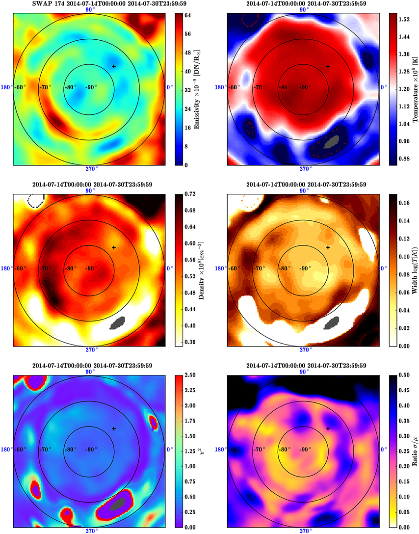
Figure 8. Same as Figure 7 but for an altitude of 1.10 R_⊙. Note that the position of the cavity center reported here (black plus sign) was measured at 1.05 R_⊙.

The bottom right panel of Figures 7, 8 represents the SWAP standard deviation-to-mean ratio σ∕μ of the emissivity computed over the 17 consecutive tomographic reconstructions (see Section 2.3). Because a 17 days windows is used for reconstructing the corona, if the cavity is completely stable in time, the standard deviation computed for each voxel at the same location, over the 17 consecutive reconstruction cubes should be small, while the artifacts and dynamic structures should present a large one. Thus, for the 14th of July reconstruction, the standard deviation and the mean have been computed through the 17 consecutive SWAP cubes spanning the observation time range from July 14 to August 16, 2014. The emissivity standard deviation-to-mean maps give us indications of the time evolution of the structures, and therefore which structures are stable in the reconstruction series. They can also be used as a way of providing uncertainties on emissivity tomographic reconstruction. This will be discussed in more details in Section 5.3.

At the height of 1.05 R_⊙, the emissivity map on top left panel of Figure 7 shows that the cavity is embedded in the quasi circular pseudostreamer observable between −70 and −60° in latitude (corresponding to orange-red structures). This is confirmed by the corresponding map of measured density (middle left panel) which is evaluated ~6.6 × 10⁷ cm⁻³ at the longitude corresponding to the central meridian of the time-centered SWAP image. In the whole cavity, the density fluctuates between ~6.4 × 10⁷ and ~8.8 × 10⁷ cm⁻³, while the density computed for the pseudostreamer is in the 1–1.1 × 10⁸ cm⁻³ range. This corresponds to a density depletion of about 20–40 %.

The corresponding temperature map is shown on top right panel of Figure 7. The area embedded within the pseudostreamer clearly exhibits higher temperatures, in the range between 1.20–1.40 MK. In particular, besides the low emissivity artifact mentioned above, the regions with lower density (see the middle left panel), are correlated with the higher temperatures, corresponding to the observable part of the cavity. Outside the closed field regions the temperature delineated by the external edge of the pseudostreamer are systematically below 1 Mk, with a mean value about 0.95 MK. The internal portion of the pseudostreamer exhibits temperatures slightly lower that the center of the cavity, with respective temperature about 1.2 and 1.35 MK, consistent with the previous AIA observations of Figure 6, discussed in Section 4. The thermal width, equivalent to the degree of multi-thermality of the voxel plasma, is lower in the cavity than in the pseudostreamer (clear areas in the middle right map of Figure 7) The pseudostreamer presents a thermal width in the range σ = 0.12 − 0.14 log T_e, while the cavity has much smaller values, around 0.04 − 0.06 log T_e. This result suggests a different heating process in both structures, with a continuous injection of energy in the cavity supplying the radiative losses, and a more sporadic heating in the pseudostreamer.

The associated normalized χ², evaluating the pertinence of the Gaussian DEM model (see Equation 11), is presented in the bottom left panel of Figure 7. The χ² values for the whole polar map are mainly concentrated around 0 and 2.50, indicating a satisfactory DEM inversion for most of the voxels. Assuming that the inferred DEMs are only affected by normally distributed random errors, the χ² DEM inversion should be equivalent to a statistical chi-squared with 3° of freedom, since we solve for the three parameters T_e, n_e, and σ. For a theoretical chi-squared 3° of freedom, the most probable value is ~1.4, which is close to the mean value of the observed map, while 95% of them are comprised between 0 and 12. This indicates that the Gaussian DEM is consistent with the observations, but this does not imply, however, that this model is the only or the best possible interpretation of the data (see Guennou et al., 2012b). It is worth noting that since the six residual χ² corresponding to the minimization process in each waveband are not completely independent, the actual chi-squared distribution will be slightly different from the expected chi-squared 3° of freedom Guennou et al. (2012a).

The corresponding emissivity standard deviation-to-mean ratio is shown in the bottom left panel of Figure 7. As can be observed, in the center of the cavity (i.e., in the neighborhood of the black plus sign) the σ∕μ ratio is between 12–16%, whereas some portions of the cavity, between 80 and 180° in longitude for example, are notably steadier, with a σ∕μ ratio close to 4%. For the pseudostreamer, the standard deviation-to-mean ratio is really high, about 40% or more, in the area comprised between 40 and 95° in longitude and −60 and −70° in latitude. This means that this part of the pseudostreamer is not stable in time, and that the signal is quite different from a reconstruction to another. Thus, these part of the map can be considered as highly uncertain.

At higher altitude, as presented in Figure 8, the pseudostreamer can still be well-observed in the SWAP emissivity map, with a quasi-circular shape, mostly located in the −70° latitude area. The cavity is identifiable as before, correlated with area of lower density embedded in the pseudostreamer. As height increases, the density decreases accordingly, both in the pseudostreamer and the cavity, with respective typical values about 6.5 × 10⁷ and 4.5 × 10⁷, corresponding to a cavity depletion of about 30%. On the other hand, the temperature increases with height in the whole map; the cavity here has a temperature about 1.45 MK whereas the external edge of the pseudostreamer is colder, with temperature around 1.2 MK. The residuals are still mostly distributed in the 0–2.5 range, with a smaller mean value than at 1.05 R_⊙, indicating, as above, a good consistency between the Gaussian DEM model and the data. The Gaussian width is also in average smaller than at lower heights, and even smaller in average in the cavity areas. However, the standard deviation is in average higher than at low heights, meaning that some temporal variations or artifacts are present. Indeed, as the height increases, strong geometrical artifacts, preventing from analyzing the structures for altitude higher than 1.15 R_⊙. They are also visible using simulations, and are geometrical effects caused by the B-angle, corresponding to the tilt of the ecliptic with respect to the solar equatorial plane (see also Barbey, 2008). Using simulations, we determined that at 1.10 R_⊙, they produce an additional error around 10–15 % in the reconstructions. This is consistent with the increase of the σ∕μ ratio of about 15% in average observed on the bottom right panel of Figure 8.

Radial properties of both the cavity and streamer are presented in Figure 9. The top and bottom panels show the temperature and density variations with respect to the altitude for both the cavity (red solid line) and the the pseudostreamer (blue solid line). The measurements are made from the constant longitude corresponding to the central meridian of the central SWAP image of the data series used for the July 14th reconstruction. The cavity center is defined as the local minimum of the latitudinal emissivity profile in the SWAP 174 Å channel (indicated by the black plus sign), while the the pseudostreamer edge is defined as the emissivity peak just equatorward of the cavity. The temperature in the cavity is slightly hotter than at the pseudostreamer edge, as the maps in Figures 7, 8 show. The density is clearly smaller in the cavity at low heights, and becomes more similar to that of the pseudostreamer at altitudes higher than 1.10 R_⊙, suggesting that the cavity extends to 1.15 R_⊙.

FIGURE 9

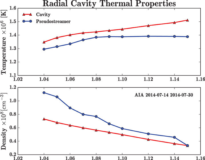
Figure 9. Radial evolution of the temperature and density with respect to the altitude in both the cavity and the pseudostreamer for the July 14th reconstruction. The temperatures are slightly higher in the cavity, while the density is clearly lower, especially at low heights.

5.2. Evolution of the Thermal Properties

Figure 10 summarizes the evolution of the local DEM parameters over the year-long lifetime of the cavity. Central temperature T_c (top panel), density n_e (second panel), thermal width σ and the χ² residuals are shown as a function of time for three different heights, at 1.05, 1.10, and 1.15 R_⊙ (using red, blue, and green solid lines, respectively). The electronic version of this journal, also contains movies corresponding to Figures 7, 8 showing the evolution of each parameter over the entire period. The reported cavity measurements in Figure 10 were made at the cavity position indicated by the black plus sign in the movie (see Section 4 for more details).

FIGURE 10

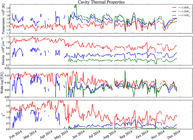
Figure 10. Evolution of the cavity Gaussian DEM parameters over the ~1-year lifetime of the cavity.

Clearly, the cavity is not well-defined at large heights until early May 2014. In Figure 10, many points for this time period are undefined, except at 1.05 R_⊙ altitude. For larger heights, strong artifacts with negative values appear in the tomographic reconstructions. This is the result of the strong dynamics of the polar structures at this period, discussed in Section 3, when irregular oscillations between streamer/pseudostreamer configurations were observed. The high values of the B-angle at this period also contribute to the uncertainty. The standard deviation-to-mean ratio is particularly high at altitudes higher than 1.10 R_⊙ during this period, confirming the presence of these artifacts (see bottom third panel in the online movies). However, it is still clear that that the mean temperature and density for this period are higher than during the shrinking phase of the pseudostreamers life. Most of the south pole has a temperature above 1.1 MK, and the highest temperatures are correlated with lowest density area (see top second and third panels of the on-line movie). The thermal width measured for this period of time is generally greater than that measured in the pseudostreamer.

Following this period, the pseudostreamer is well established and starts to shrink. As can be observed on the online movies, the pseudostreamer volume systematically presents temperatures higher than 1.15, 1.20, and 1.35 MK for the respective altitudes of 1.05, 1.10, and 1.15 R_⊙. Outside the pseudostreamer, the temperature is always below 1 MK, corresponding to typical temperatures measured in the open field coronal holes. Inside the pseudostreamer volume, higher temperatures are observed. The cavity itself has the highest temperature, and the lowest local density measurements. The shrinking of the pseudostreamer is well observable in each of the local DEM parameters. The high-temperature quasi-circular region corresponding to the pseudostreamer system is clearly reduced with time, corresponding to the pseudostreamer morphology observed in the SWAP emissivity map. The mean density of the whole south pole slowly decreases with time, and the cavity is easily identifiable as the lowest density central area, slowly drifting toward the pole. While the pseudostreamer shrinks, the mean thermal width of the whole south pole slowly decreases. The χ² residuals exhibit smaller values than the early 2014 reconstructions, indicating a better agreement between the Gaussian DEM model and the data. This is consistent with the increased stability of the pseudostreamer for this period, leading to better reconstruction quality. Accordingly, the σ∕μ ratio is, on average, smaller for this time interval.

According to Figure 10, two regimes can be observed within the cavity, at least at low height. During the first 5 months before the pseudostreamer starts to shrink, the cavity temperature, density and thermal width measured at 1.05 R_⊙ (red solid line) are quite stable, with respective values of about 1.25 MK, 1 × 10⁸ cm⁻³ and 0.14 log T_e. However, once the pseudostreamer shrinks, the density, thermal width and the χ² slowly decrease until July, 2014, while the temperature stays stable. At 1.05 R_⊙, the mean density settles at about 0.8 × 10⁸ cm⁻³, the thermal width about 0.08 log T_e and the χ² decreases from the 1.5–2.5 to the 0.4–1.4 range. At greater heights, the first regime is not observable due to the lack of data during the January-May interval. Nevertheless, the second regime, during the shrinking process of the pseudostreamer, i.e., after May 2014, is well-observable and the density, thermal width and χ² remains mostly stable. This stability is likely a result of the fact that, except when the pseudostreamer is very large early in its lifetime, the location at 1.15 R_⊙ is in the open field polar coronal hole. The temperature, especially at 1.15 R_⊙ fluctuates somewhat, most probably due to the artifacts generated at large heights.

5.3. Uncertainties

There are a number of uncertainties affecting the results. SWAP and AIA observations are mostly subject to random errors, caused by both Poisson photon noise and detection noises, such as dark current-induced electron shot noise and read noise. This noise can be reduced by the median- and average-stacking done on the individual frames used in each reconstruction. The reconstructed emissivities are then affected by the errors involved in the reconstruction process, such as the temporal variation of the corona, or the geometrical artifacts discussed in the Section 5 like differential rotation. TomograPy uses the Baye's formalism, assuming a statistical Gaussian noise affecting the data. In this framework, the uncertainties associated with the observational noises are provided by the covariance matrix. Unfortunately, in most practical case, the covariance is too big to be kept in memory (see Barbey et al., 2013, for more details). Comparatively, the random errors involved in the SWAP and AIA data are more likely to be smaller than in comparison to the uncertainties associated with the tomographic reconstruction process, and can be neglected.

Quantifying how much the time variation of the corona affects the reconstruction is not trivial and is beyond the scope of this paper. However, the standard deviation-to-mean ratio, σ∕μ described in Section 5 can give us an estimate of the degree of temporal variation. Inspecting the online movie showing the SWAP polar caps and the associated σ∕μ ratio, we can derive an upper limit on the emissivity uncertainty, at least for the steady lifetime of the pseudostreamer system (i.e., from May to December 2015). For the altitudes of 1.05, 1.10, 1.15 R_⊙, the standard deviation-to-mean ratio generally does not exceed—except in some rare cases—values of about 15, 20, and 25%, respectively. These values will be considered as the upper limit of the emissivity uncertainties in the following discussion.

The local DEM is estimated from the AIA multi-wavelength emissivities computed using a second inversion process. Aside from the classical difficulties inherent to inverse problems, the systematic errors involved in the AIA instrument calibration and in the atomic physics systematically skew the interpretation of the measured emissivity in the same direction. The calibration involves a complex chain of measurements, from which the uncertainties are difficult to deduce. Initially estimated to 25%, the AIA calibration error was reduced to 10% by Boerner et al. (2014) after applying the cross-calibration. Errors associated with atomic physics are a major source of uncertainty the DEM inversion problem. Missing atomic transitions, especially for the 94 and 131 Å observations, underestimate the signal observed. The assumption of ionization equilibrium can also be invalid in some cases, affecting the calculated transition rates. Abundances uncertainties, and variations along the LOS also impact the interpretation of the observations, particularly in the corona where the first ionization effect (FIP) takes place in some structures.

Effects of both calibration and atomic physics uncertainties on the robustness of the AIA Gaussian DEM inversion have been studied in detail by Guennou et al. (2012a) and Guennou et al. (2012b). Based on a Bayesian interpretation of Monte-Carlo simulations, the authors determined how much the AIA Gaussian DEM inversion is affected by the uncertainties. In these previous studies, both types of errors are estimated at 25%, and detection noise is considered, although the latter are mostly negligible in comparison with the systematics. From the probability distributions computed by the authors, the uncertainties associated to the measured DEM parameters can be derived (see Guennou et al., 2013, for a practical example). Authors showed that it is possible to reconstruct simple DEMs with AIA data, but that the accuracy of the results decreases with respect to the thermal width of the plasma.

In this present work, we assume the following: 10% error for the calibration, 25% error for atomic physics, and a reconstruction noise that varies between 15 and 25% depending on altitude. This leads to a total uncertainty between 30 and 36% in the present DEM inversions, which is quite similar to the total 35% uncertainty reported by Guennou et al. (2012b). The thermal width at the south pole never exceeds 0.2 log T_e, in the results presented here. Moreover, during the stable lifetime of the pseudostreamer, the thermal width is typically in the range of 0.06–0.09 log T_e. For these characteristic intervals of the thermal width, Guennou et al. (2012b) showed that the AIA Gaussian inversion is robust, although some secondary solutions, can appear with low probability. For isothermal plasma in the temperature range of about 1 MK, authors found that the temperature resolution is proportional to the total uncertainty level σ_unc as $\Delta T_c^P~0.15{\sigma }_{unc}$. Using the probability maps, given a maximum thermal width of σ = 0.02 log T_e and taking σ_unc = 35%, we find an upper limit on the temperature resolution of ΔT_c = 0.075 log T_e. The density is better constrained, with an upper limit estimated at Δn_e = 0.055 log n_e. These estimations have been made by adopting a rigorous approach to uncertainties in the DEM inversion problem. However, the emissivity uncertainties, given by the standard deviation-to-mean ratio can be higher locally, especially when artifacts are present.

6. Discussion

6.1. Pseudostreamer and Cavity Density

In our results, the cavity is clearly less dense than the surrounding pseudostreamer. The cavity depletion, relative to the surrounding pseudostreamer varies in the range of 20–40% at 1.05 R_⊙, depending on the period studied. These results are consistent with previous EUV and white-light studies, which have unambiguously established the presence of density depletion within cavity (see e.g., Gibson and Fan, 2006; Fuller and Gibson, 2009; Kucera et al., 2012, and references therein). Our observations reveal that the density depletion decreases with height, as shown by the density profile in Figure 9. These results are also in agreement with the density profiles measured by Fuller et al. (2008), where the density depletion in a white-light cavity is maximum at low altitude and decreases to practically nothing at the cavity top.

Lower density in cavities can be expected in the case that the magnetic field dramatically changes at the cavity boundaries due to a current sheet or layer. The conservation of the total pressure leads to a reduction in thermal pressure to counter the magnetic pressure increase within the cavity. If the temperature is not significantly different between the cavity and its surroundings, as this is the case in our results (see Section 6.2), the pressure change leads to a density depletion. According to Gibson and Fan (2006), even if the axial field change at the cavity boundaries is very small, it still results in a strong jump in thermal pressure and a current sheet does form, a scenario consistent with the generally distinct elliptical boundaries of cavities. The density depletion observed in the center of the cavity is still not fully understood, though some compelling hypotheses exist (Gibson et al., 2010; Schmit et al., 2013).

The magnetic structure, and in particular the magnetic field length, induces some thermodynamic variations, which in turn lead to density depletion within the cavity. For a flux rope cavity model, the integration along the LOS of longer field line, carrying more particles than the shorter one, results in higher observed density (Krall and Chen, 2005). By resolving the hydrostatic equilibrium along the flux rope magnetic field lines, Schmit and Gibson (2011) show that short axial field lines would be depleted by a factor about 35%. Significant thermal non-equilibrium effects can also take place for the longer field line (Klimchuk et al., 2010). Additionally, the degree of twist of the flux rope is an important parameter controlling the amount of density depletion within the cavity (Gibson et al., 2010). Therefore, our measurements of the cavities 3D morphology, together with the density and temperature profiles can help to constrain the flux rope twist and arch.

6.2. Pseudostreamer and Cavity Temperature

Our results clearly show that the volume enclosed within the pseudostreamer is systematically hotter than the plasma outside of it, a feature which is observed during the entire pseudostreamer lifetime. This volume systematically presents temperatures higher than 1.15, 1.20, and 1.35 MK for the respective altitudes of 1.05, 1.10, and 1.15 R_⊙. The outermost temperature is always below 1 MK, corresponding to typical temperatures measured in the open field coronal holes. Examining the fine temperature distribution of the internal portion of the pseudostreamer, we found that the area corresponding to the lowest local density are correlated with the hottest temperature. The difference is small though, with 1.2 MK in most of the pseudostreamer vs. 1.35 MK within the cavity at 1.05 R_⊙ for the July 14th reconstruction presented in Section 5.

However, taking the upper limit temperature uncertainties to be about 0.075 log T_e as discussed in Section 5.3, the pseudostreamer/cavity temperatures become ${1.2}_{-0.19}^{+0.22}$ and ${1.35}_{-0.21}^{+0.25}$ MK, and the difference is within the error bars. In spite of that, given the predominantly systematic nature of the source of the uncertainties, the results are likely to be pushed all together in the same direction. Therefore, the difference is most probably to be significant, even though a formal conclusion is not possible. Efforts are needed to reduce the uncertainty sources, which will be a significant task in and of itself.

The temperature profile of coronal cavities is still an open question. Previous analyses resulted in conflicting results, some authors arguing that cavities are hotter (Fuller et al., 2008; Vásquez et al., 2009; Habbal et al., 2010), whereas Guhathakurta et al. (1992) found them cooler. Using a combination of Hinode/EIS and M4K coronameter data, Kucera et al. (2012) concluded that streamer and cavity have essentially the same temperature. They found a temperature profile of about 1.4 MK at 1.04 R_⊙ to about 1.6 MK at 1.14–1.16 R_⊙ in both the surrounding streamer and the cavity. This is, given the uncertainties, consistent with our temperature profiles presented in Figure 9.

The hot central core of the cavities, referred as the “chewy nougat” can sometimes be observed in soft X-rays (Hudson et al., 1999) and persist for the lifetime of the cavity. The hot core has a roughly tube-like shape, suspended above the base of the cavity (Reeves et al., 2012). They are suspected to be the result of current sheet formation and associated reconnection at the flux rope base. We do not observe any similar temperature increase in our reconstructions, even in the AIA channels sensible to high temperatures (94, 131, and 193 Å). It could be due to the transitory nature of these “chewy nougat” events, for which the tomography timescale is too extensive to resolve. However, this is consistent with Vial and Engvold (2015), mentioning in their cavity review that there is not, generally, a corresponding signature to the hot core in EUV wavelengths.

Temperature variations in the cavity are most likely correlated with the magnetic structure. Temperature measurements are thus improved by knowledge of the 3D morphology, to separate potential projection effects. Therefore, our results, in combination with cavity models and simulations, can be very useful in providing strong constraints on the processes that maintain cavity stability for long periods of time.

6.3. Evolution of the Pseudostreamer/Cavity System

Two regimes in the pseudostreamer/cavity system are clearly discernible—at least at low heights. During the January—May 2014 interval, the pseudostreamer seems to oscillate between streamer/pseudostreamer configuration, making the tomographic reconstructions more difficult to achieve, highlighted by the higher values of both the χ² and standard deviation to mean ratio higher values. However, we can clearly note that, the density and the thermal width are higher for this time period, and that the entire south pole is at temperature higher than 1.1 MK, indicating that no open field lines configuration are present. The thermal width is, on average, higher in the low density areas, corresponding to the cavity, than it is in the pseudostreamer features.

Once the pseudostreamer is clearly established and therefore in a more steady state, it starts to slowly shrink. The temperature of the pseudostreamer/cavity system, remains, on average, stable meanwhile the shrinking is occurring. By contrast, the density slowly decreases with time within the pseudostreamer/cavity system. At 1.05 R_⊙, the cavity density is around 1.1 × 10⁸ cm⁻³ in January 2014 and 0.8 × 10⁸ cm⁻³ in December 2015. At higher altitudes, a similar trend can be noted, even though both the intense pseudostreamer dynamics and geometric artifacts highly limits the tomographic reconstructions interpretation in the first 5 months of 2014. The thermal width is distinctly smaller than in the first semester 2014, with values decreasing from about 0.15 to about 0.07 × log T_e. On the other hand, the cavity thermal width exhibits lower values in average than that of the pseudostreamer, an opposite behavior to that observed in the first part of 2014.

If previous studies did not converge toward a non-ambiguous answer to the cavity temperature question, most authors found more thermal variability in the cavity plasma than in the surrounding corona. In our results, this occurs only during the first half lifetime of the cavity. As we mentioned previously, the thermodynamic properties of the plasma can vary significantly, depending on the magnetic field line length and curvature. Therefore, this change could be related to a reorganization in the magnetic configuration in the south pole. This investigation is beyond the scope of the present paper, but comparison between magnetic field extrapolation and our tomographic reconstructions are planned in a future work.

7. Summary

In this work, we present a full analysis of an exceptional long-lived pseudostreamer/cavity system, observable for almost a year, starting in February 2014. We used SWAP data and 6 AIA coronal wavebands to study its evolution, examining both its 3D morphology and thermodynamical properties. At first, a streamer encircles the entire pole, associated with a polar-crown cavity. By dint of a gradual displacement toward the south pole, a pseudostreamer is formed above the south pole in February 2014, which remains visible for approximately a year. Following that, the pseudostreamer gradually shrink until its disappearance in March 2015, at which point the southern polar coronal hole once again dominates the pole.

We used a combination of tomography and DEM analysis to track the evolution of the 3D thermodynamical properties of this unusually long-lived pseudostreamer/cavity system. Tomography is used to recover the three-dimensional emission of the plasma using multiple EUV wavelengths, allowing us to determine the south pole morphology. From these multi-wavelength 3D observations, we then derive the plasma density, temperature and thermal distribution for each location in space, using the DEM formalism.

The dynamic nature of the corona, as cavity swirling motions (Wang and Stenborg, 2010) or rising bubbles, plumes and flows in prominences (Schmit et al., 2013) may complicate our tomographic analyses, which assume no time variations during the 17 days of acquisition. In this work, we chose to only focus on the stable coronal structures in our reconstructions, instead dynamic and eruptive events which in turn increase the degree of under-determination of the inverse problem. For our time-analysis we used a 1 day sliding-window in time, and then constructed standard deviation-to-mean ratio over successive reconstructions. This allow us to discriminate static structures from the temporal and geometrical artifacts, and ensure that the observed features in our reconstructions are real. To our knowledge, this is the first time that this kind of approach has been used to analyze tomographic reconstructions.

Our results are summarized as follows:

• The cavity depletion, relative to the surrounding pseudostreamer varies in the range of 20–40% depending on height,

• The cavity density depletion decreases with height, from a maximum of about 40% at the cavity lower boundary to ~0% at the cavity top,

• The cavity density slowly decreases with time as the pseudostreamer shrinks,

• The volume enclosed within the pseudostreamer is systematically hotter than the surrounding open-field plasma,

• The cavity temperature is essentially at similar or slightly higher temperatures than the pseudostreamer,

• No cavity hot cores were observed in our dataset,

• Two regimes in cavity density and thermal distribution are observable during the pseudostreamer lifetime. The January-June 2014 interval corresponds to the highest cavity density values, while the thermal distribution is higher in cavity than in the pseudostreamer. Afterwards, the cavity density and the thermal width both decrease.

These results, used in combination with pseudostreamer/cavity models, can give us important information about magnetic configuration, a meaningful parameter to understand both the origin of CMEs and the processes that maintain cavity stability for such long periods of time. Thermodynamic properties being strongly correlated to the magnetic structure, our measurements of the cavities 3D morphology, together with the density and temperature profiles can help to constrain the flux rope twist and arch.

Author Contributions

The works was mainly done by CG. CG performed all the tomographic reconstructions, the local DEM inversions, prepared the AIA data, and anylyzed and interpreted the results. LR analyzed the SWAP, compared with magnetograms, and interpret the data from the magnetic point of view. DS prepared the SWAP data and helped during the writing process. FA participated to the tomographic reconstructions, and helped in their interpretation, in particular for the understanding of the geometric artifacts.

Conflict of Interest Statement

The authors declare that the research was conducted in the absence of any commercial or financial relationships that could be construed as a potential conflict of interest.

Acknowledgments

CG acknowledges financial support from the Spanish Ministry of Economy and Competitiveness (MINECO) under the 2011 Severo Ochoa Program MINECO SEV-2011-0187. The authors would like to thank the technical staff at the Computer Science Department of the Institut d'Astrophysique Spatiale, Orsay, France, for allowing us to use their computational facilities. CG would like to thank in particular Claude Mercier and Elie soubrié for helpful suggestions in the DEM inversion code parallelization. The Atmospheric Imaging Assembly on the Solar Dynamics Observatory is part of NASA's Living with a Star program. CHIANTI is a collaborative project involving the NRL (USA), the Universities of Florence (Italy) and Cambridge (UK), and George Mason University (USA). LR and DS acknowledge support from the Belgian Federal Science Policy Office (BELSPO) through the ESA-PRODEX program, grant No. 4000103240. SWAP is a project of the Centre Spatial de Liege and the Royal Observatory of Belgium funded by BELSPO.

Footnotes

1. ^https://pypi.python.org

References

Abbo, L., Lionello, R., Riley, P., and Wang, Y.-M. (2015). Coronal pseudo-streamer and bipolar streamer observed by SOHO/UVCS in March 2008. Sol. Phys. 290, 2043–2054. doi: 10.1007/s11207-015-0723-y

CrossRef Full Text | Google Scholar

Altrock, R. C. (2003). A study of the rotation of the solar corona. Sol. Phys. 213, 23–37. doi: 10.1023/A:1023204814099

CrossRef Full Text | Google Scholar

Aschwanden, M. J. (2011). Solar stereoscopy and tomography. Living Rev. Sol. Phys. 8:5. doi: 10.12942/lrsp-2011-5

CrossRef Full Text | Google Scholar

Auchère, F., Guennou, C., and Barbey, N. (2012). “Tomographic reconstruction of polar plumes,” in EAS Publications Series, Volume 55 of EAS Publications Series, eds M. Faurobert, C. Fang, and T. Corbard, 207–211. Available online at: http://cdsads.u-strasbg.fr/abs/2012EAS….55.207A

Barbey, N. (2008). Determination of the Tridimensional Structures of the Solar Corona Using Data from the SoHO and STEREO missions. Theses, Université Paris Sud - Paris XI.

Barbey, N., Auchère, F., Rodet, T., and Vial, J.-C. (2008). A time-evolving 3D method dedicated to the reconstruction of solar plumes and results using extreme ultraviolet data. Sol. Phys. 248, 409–423. doi: 10.1007/s11207-008-9151-6

CrossRef Full Text | Google Scholar

Barbey, N., Guennou, C., and Auchère, F. (2013). TomograPy: a fast, instrument-independent, solar tomography software. Sol. Phys. 283, 227–245. doi: 10.1007/s11207-011-9792-8

CrossRef Full Text | Google Scholar

Boerner, P. F., Testa, P., Warren, H., Weber, M. A., and Schrijver, C. J. (2014). Photometric and thermal cross-calibration of solar EUV instruments. Sol. Phys. 289, 2377–2397. doi: 10.1007/s11207-013-0452-z

CrossRef Full Text | Google Scholar

Borovsky, J. E., and Denton, M. H. (2013). The differences between storms driven by helmet streamer CIRs and storms driven by pseudostreamer CIRs. J. Geophys. Res. Space Phys., 118, 5506–5521. doi: 10.1002/jgra.50524

CrossRef Full Text | Google Scholar

Borrini, G., Wilcox, J. M., Gosling, J. T., Bame, S. J., and Feldman, W. C. (1981). Solar wind helium and hydrogen structure near the heliospheric current sheet - A signal of coronal streamers at 1 AU. J. Geophys. Res. 86, 4565–4573. doi: 10.1029/JA086iA06p04565

CrossRef Full Text | Google Scholar

Brown, J. C., Dwivedi, B. N., Sweet, P. A., and Almleaky, Y. M. (1991). The interpretation of density sensitive line diagnostics from inhomogeneous plasmas. II - Non-isothermal plasmas. Astron. Astrophys. 249, 277–283.

Google Scholar

Butala, M. D., Hewett, R. J., Frazin, R. A., and Kamalabadi, F. (2010). Dynamic three-dimensional tomography of the solar corona. Sol. Phys. 262, 495–509. doi: 10.1007/s11207-010-9536-1

CrossRef Full Text | Google Scholar

Cheung, M. C. M., Boerner, P., Schrijver, C. J., Testa, P., Chen, F., Peter, H., et al. (2015). Thermal diagnostics with the atmospheric imaging assembly on board the solar dynamics observatory: a validated method for differential emission measure inversions. Astrophys. J. 807, 143. doi: 10.1088/0004-637X/807/2/143

CrossRef Full Text | Google Scholar

Craig, I. J. D., and Brown, J. C. (1976). Fundamental limitations of X-ray spectra as diagnostics of plasma temperature structure. Astron. Astrophys. 49, 239–250.

Google Scholar

de Patoul, J., Inhester, B., Feng, L., and Wiegelmann, T. (2013). 2D and 3D polar plume analysis from the three vantage positions of STEREO/EUVI A, B, and SOHO/EIT. Sol. Phys. 283, 207–225. doi: 10.1007/s11207-011-9902-7

CrossRef Full Text | Google Scholar

Dere, K. P., Landi, E., Mason, H. E., Monsignori Fossi, B. C., and Young, P. R. (1997). CHIANTI - an atomic database for emission lines. Astron. Astrophys. Suppl. Ser. 125, 149–173. doi: 10.1051/aas:1997368

CrossRef Full Text | Google Scholar

Eselevich, V. G., and Tong, Y. (1997). New results on the site of initiation of coronal mass ejections and an interpretation of observation of their interaction with streamers. J. Geophys. Res. 102, 4681–4690. doi: 10.1029/96JA02875

CrossRef Full Text | Google Scholar

Frazin, R. A. (2000). Tomography of the solar corona. I. A robust, regularized, positive estimation method. Astrophys. J. 530, 1026–1035. doi: 10.1086/308412

CrossRef Full Text | Google Scholar

Frazin, R. A., Butala, M. D., Kemball, A., and Kamalabadi, F. (2005a). Time-dependent reconstruction of nonstationary objects with tomographic or interferometric measurements. Astrophys. J. Lett. 635, L197–L200. doi: 10.1086/499431

PubMed Abstract | CrossRef Full Text | Google Scholar

Frazin, R. A., and Janzen, P. (2002). Tomography of the solar corona. II. Robust, regularized, positive estimation of the three-dimensional electron density distribution from LASCO-C2 polarized white-light images. Astrophys. J. 570, 408–422. doi: 10.1086/339572

CrossRef Full Text | Google Scholar

Frazin, R. A., Kamalabadi, F., and Weber, M. A. (2005b). On the combination of differential emission measure analysis and rotational tomography for three-dimensional solar EUV imaging. Astrophys. J. 628, 1070–1080. doi: 10.1086/431295

CrossRef Full Text | Google Scholar

Frazin, R. A., Vásquez, A. M., and Kamalabadi, F. (2009). Quantitative, three-dimensional analysis of the global corona with multi-spacecraft differential emission measure tomography. Astrophys. J. 701, 547–560. doi: 10.1088/0004-637X/701/1/547

CrossRef Full Text | Google Scholar

Fuller, J., and Gibson, S. E. (2009). A survey of coronal cavity density profiles. Astrophys. J. 700, 1205–1215. doi: 10.1088/0004-637X/700/2/1205

CrossRef Full Text | Google Scholar

Fuller, J., Gibson, S. E., de Toma, G., and Fan, Y. (2008). Observing the unobservable? Modeling coronal cavity densities. Astrophys. J. 678, 515–530. doi: 10.1086/533527

CrossRef Full Text | Google Scholar

Gibson, S. E., and Fan, Y. (2006). Coronal prominence structure and dynamics: a magnetic flux rope interpretation. J. Geophys. Res. Space Phys.) 111, 12103. doi: 10.1029/2006ja011871

CrossRef Full Text | Google Scholar

Gibson, S. E., Kucera, T. A., Rastawicki, D., Dove, J., de Toma, G., Hao, J., et al. (2010). Three-dimensional morphology of a coronal prominence cavity. Astrophys. J. 724, 1133–1146. doi: 10.1088/0004-637X/724/2/1133

CrossRef Full Text | Google Scholar

Guennou, C., Auchère, F., Klimchuk, J. A., Bocchialini, K., and Parenti, S. (2013). Can the differential emission measure constrain the timescale of energy deposition in the corona? Astrophys. J. 774, 31. doi: 10.1088/0004-637X/774/1/31

CrossRef Full Text | Google Scholar

Guennou, C., Auchère, F., Soubrié, E., Bocchialini, K., Parenti, S., and Barbey, N. (2012a). On the accuracy of the differential emission measure diagnostics of solar plasmas. Application to SDO/AIA. I. Isothermal plasmas. Astrophys. J. Suppl. Ser. 203, 25. doi: 10.1088/0067-0049/203/2/25

CrossRef Full Text | Google Scholar

Guennou, C., Auchère, F., Soubrié, E., Bocchialini, K., Parenti, S., and Barbey, N. (2012b). On the accuracy of the differential emission measure diagnostics of solar plasmas. Application to SDO/AIA. II. Multithermal plasmas. Astrophys. J. Suppl. Ser. 203, 26. doi: 10.1088/0067-0049/203/2/26

CrossRef Full Text | Google Scholar

Guhathakurta, M., Rottman, G. J., Fisher, R. R., Orrall, F. Q., and Altrock, R. C. (1992). Coronal density and temperature structure from coordinated observations associated with the total solar eclipse of 1988 March 18. Astrophys. J. 388, 633–643. doi: 10.1086/171180

CrossRef Full Text | Google Scholar

Habbal, S. R., Druckmüller, M., Morgan, H., Scholl, I., Rušin, V., Daw, A., et al. (2010). Total solar eclipse observations of hot prominence shrouds. Astrophys. J. 719, 1362–1369. doi: 10.1088/0004-637X/719/2/1362

CrossRef Full Text | Google Scholar

Halain, J.-P., Berghmans, D., Seaton, D. B., Nicula, B., De Groof, A., Mierla, M., et al. (2013). The SWAP EUV imaging telescope. Part II: in-flight performance and calibration. Sol. Phys. 286, 67–91. doi: 10.1007/s11207-012-0183-6

CrossRef Full Text | Google Scholar

Hannah, I. G., and Kontar, E. P. (2012). Differential emission measures from the regularized inversion of Hinode and SDO data. Astron. Astrophys. 539:A146. doi: 10.1051/0004-6361/201117576

CrossRef Full Text | Google Scholar

Higdon, D. M., Bowsher, J. E., Johnson, V. E., Turkington, T. G., Gilland, D. R., and Jaszczak, R. J. (1997). Fully bayesian estimation of Gibbs hyperparameters for emission computed tomography data. IEEE Trans. Med. Imaging 16, 516–526. doi: 10.1109/42.640741

PubMed Abstract | CrossRef Full Text | Google Scholar

Howard, R. A., Sheeley, Jr. N. R., Michels, D. J., and Koomen, M. J. (1985). Coronal mass ejections - 1979-1981. J. Geophys. Res. 90, 8173–8191. doi: 10.1029/JA090iA09p08173

CrossRef Full Text | Google Scholar

Huang, Z., Frazin, R. A., Landi, E., Manchester, W. B., Vásquez, A. M., and Gombosi, T. I. (2012). Newly discovered global temperature structures in the quiet sun at solar minimum. Astrophys. J. 755, 86. doi: 10.1088/0004-637X/755/2/86

CrossRef Full Text | Google Scholar

Hudson, H. S., Acton, L. W., Harvey, K. L., and McKenzie, D. E. (1999). A stable filament cavity with a hot core. Astrophys. J. Lett. 513, L83–L86. doi: 10.1086/311892

CrossRef Full Text | Google Scholar

Jefferies, J. T., Orrall, F. Q., and Zirker, J. B. (1972). The interpretation of total line intensities from optically thin gases. I: a general method. Sol. Phys. 22, 307–316. doi: 10.1007/BF00148698

CrossRef Full Text | Google Scholar

Judge, P. G., Hubeny, V., and Brown, J. C. (1997). Fundamental limitations of emission-line spectra as diagnostics of plasma temperature and density structure. Astrophys. J. 475, 275–290. doi: 10.1086/303511

CrossRef Full Text | Google Scholar

Kashyap, V., and Drake, J. J. (1998). Markov-Chain Monte Carlo reconstruction of emission measure distributions: application to solar extreme-ultraviolet spectra. Astrophys. J. 503, 450–466. doi: 10.1086/305964

CrossRef Full Text | Google Scholar

Klimchuk, J. A., Karpen, J. T., and Antiochos, S. K. (2010). Can thermal nonequilibrium explain coronal loops? Astrophys. J. 714, 1239–1248. doi: 10.1088/0004-637X/714/2/1239

CrossRef Full Text | Google Scholar

Krall, J., and Chen, J. (2005). Density structure of a preeruption coronal flux rope. Astrophys. J. 628, 1046–1055. doi: 10.1086/430810

CrossRef Full Text | Google Scholar

Kucera, T. A., Gibson, S. E., Schmit, D. J., Landi, E., and Tripathi, D. (2012). Temperature and extreme-ultraviolet intensity in a coronal prominence cavity and streamer. Astrophys. J. 757:73. doi: 10.1088/0004-637X/757/1/73

CrossRef Full Text | Google Scholar

Landi, E., Young, P. R., Dere, K. P., Del Zanna, G., and Mason, H. E. (2013). CHIANTI - an atomic database for emission lines. XIII. soft X-Ray improvements and other changes. Astrophys. J. 763:86. doi: 10.1088/0004-637X/763/2/86

CrossRef Full Text | Google Scholar

Lynch, B. J., and Edmondson, J. K. (2013). Sympathetic magnetic breakout coronal mass ejections from pseudostreamers. Astrophys. J. 764:87. doi: 10.1088/0004-637X/764/1/87

CrossRef Full Text | Google Scholar

Marqué, C. (2004). Radio metric observations of quiescent filament cavities. Astrophys. J. 602, 1037–1050. doi: 10.1086/381085

CrossRef Full Text | Google Scholar

Mason, H. E., and Fossi, B. C. M. (1994). Spectroscopic diagnostics in the VUV for solar and stellar plasmas. Astron. Astrophys. Rev. 6, 123–179. doi: 10.1007/BF01208253

CrossRef Full Text | Google Scholar

Nuevo, F. A., Huang, Z., Frazin, R., Manchester, IV, W. B., Jin, M., and Vásquez, A. M. (2013). Evolution of the global temperature structure of the solar corona during the minimum between solar cycles 23 and 24. Astrophys. J. 773:9. doi: 10.1088/0004-637X/773/1/9

CrossRef Full Text | Google Scholar

Nuevo, F. A., Vásquez, A. M., Landi, E., and Frazin, R. (2015). Multimodal differential emission measure in the solar corona. Astrophys. J. 811:128. doi: 10.1088/0004-637X/811/2/128

CrossRef Full Text | Google Scholar

Pottasch, S. R. (1963). The lower solar corona: interpretation of the ultraviolet spectrum. Astrophys. J. 137:945. doi: 10.1086/147569

CrossRef Full Text | Google Scholar

Rachmeler, L. A., Platten, S. J., Bethge, C., Seaton, D. B., and Yeates, A. R. (2014). Observations of a hybrid double-streamer/pseudostreamer in the solar corona. Astrophys. J. Lett. 787:L3. doi: 10.1088/2041-8205/787/1/L3

CrossRef Full Text | Google Scholar

Reeves, K. K., Gibson, S. E., Kucera, T. A., Hudson, H. S., and Kano, R. (2012). Thermal properties of a solar coronal cavity observed with the X-Ray telescope on hinode. Astrophys. J. 746:146. doi: 10.1088/0004-637X/746/2/146

CrossRef Full Text | Google Scholar

Schmit, D. J., Gibson, S., Luna, M., Karpen, J., and Innes, D. (2013). Prominence mass supply and the cavity. Astrophys. J. 779:156. doi: 10.1088/0004-637X/779/2/156

CrossRef Full Text | Google Scholar

Schmit, D. J., and Gibson, S. E. (2011). Forward modeling cavity density: a multi-instrument diagnostic. Astrophys. J. 733:1. doi: 10.1088/0004-637X/733/1/1

CrossRef Full Text | Google Scholar

Seaton, D. B., Berghmans, D., Nicula, B., Halain, J.-P., De Groof, A., Thibert, T., et al. (2013). The SWAP EUV imaging telescope part I: instrument overview and pre-flight testing. Sol. Phys. 286, 43–65. doi: 10.1007/s11207-012-0114-6

CrossRef Full Text

Siddon, R. L. (1985). Prism representation: a 3D ray-tracing algorithm for radiotherapy applications. Phys. Med. Biol. 30, 817–824. doi: 10.1088/0031-9155/30/8/005

PubMed Abstract | CrossRef Full Text | Google Scholar

Sturrock, P. A., and Smith, S. M. (1968). Magnetic-field structure associated with coronal streamers. Sol. Phys. 5, 87–101. doi: 10.1007/BF00147122

CrossRef Full Text | Google Scholar

Testa, P., De Pontieu, B., Martínez-Sykora, J., Hansteen, V., and Carlsson, M. (2012). Investigating the reliability of coronal emission measure distribution diagnostics using three-dimensional radiative magnetohydrodynamic simulations. Astrophys. J. 758:54. doi: 10.1088/0004-637X/758/1/54

CrossRef Full Text | Google Scholar

Vásquez, A. M., Frazin, R. A., and Kamalabadi, F. (2009). 3D temperatures and densities of the solar corona via multi-spacecraft EUV tomography: analysis of prominence cavities. Sol. Phys. 256, 73–85. doi: 10.1007/s11207-009-9321-1

CrossRef Full Text | Google Scholar

Vial, J.-C., and Engvold, O. (eds.). (2015). Solar Prominences, Vol. 415 of Astrophysics and Space Science Library. Springer International Publishing. Available online at: http://www.springer.com/us/book/9783319104157

Wang, Y.-M. (2015). Pseudostreamers as the source of a separate class of solar coronal mass ejections. Astrophys. J. Lett. 803:L12. doi: 10.1088/2041-8205/803/1/L12

CrossRef Full Text | Google Scholar

Wang, Y.-M., Sheeley, Jr. N. R., Nash, A. G., and Shampine, L. R. (1988). The quasi-rigid rotation of coronal magnetic fields. Astrophys. J. 327, 427–450. doi: 10.1086/166205

CrossRef Full Text | Google Scholar

Wang, Y.-M., Sheeley, Jr. N. R., and Rich, N. B. (2007). Coronal Pseudostreamers. Astrophys. J. 658, 1340–1348. doi: 10.1086/511416

CrossRef Full Text | Google Scholar

Wang, Y.-M., and Stenborg, G. (2010). Spinning motions in coronal cavities. Astrophys. J. 719, L181–L184. doi: 10.1088/2041-8205/719/2/l181

CrossRef Full Text | Google Scholar

Wuelser, J.-P., Lemen, J. R., Tarbell, T. D., Wolfson, C. J., Cannon, J. C., Carpenter, B. A., et al. (2004). “EUVI: the STEREO-SECCHI extreme ultraviolet imager,” in Telescopes and Instrumentation for Solar Astrophysics, Volume 5171 of Proceedings of the SPIE, eds S. Fineschi and M. A. Gummin, 111–122. Available online at: http://cdsads.u-strasbg.fr/abs/2004SPIE.5171..111W

Zhao, L., Gibson, S. E., and Fisk, L. A. (2013). Association of solar wind proton flux extremes with pseudostreamers. J. Geophys. Res. Space Phys. 118, 2834–2841. doi: 10.1002/jgra.50335

CrossRef Full Text | Google Scholar

Zhao, X. P., and Webb, D. F. (2003). Source regions and storm effectiveness of frontside full halo coronal mass ejections. J. Geophys. Res. Space Phys. 108:1234. doi: 10.1029/2002JA009606

CrossRef Full Text | Google Scholar