ROAM: A Radial-Basis-Function Optimization Approximation Method for Diagnosing the Three-Dimensional Coronal Magnetic Field

1. Introduction

Modification to the polarization of light is one of the many signatures of a non-zero magnetic field in the solar corona, and more generally, in the solar atmosphere (e.g., Stenflo, 2015, and references therein). Several mechanisms producing or modifying the polarization of light have been observed and studied in the solar corona at different wavelengths including, but not limited to, the Zeeman and Hanle effects (see e.g., Hale, 1908; Hanle, 1924; Bird et al., 1985; White and Kundu, 1997; Casini and Judge, 1999; Lin et al., 2004; Gibson et al., 2016, and references therein). The former induces a frequency-modulated polarization while the latter induces a depolarization of scattered light (e.g., Sahal-Brechot et al., 1977; Bommier and Sahal-Brechot, 1982; Rachmeler et al., 2013; López Ariste, 2015). Both mechanisms allow us to probe the strength and direction of the coronal magnetic field. Coronal polarization associated with these two mechanisms is currently measured above the solar limb by the Coronal Multichannel Polarimeter from forbidden coronal lines such as the Fe XIII lines (10747 Å and 10798 Å; Tomczyk et al., 2008). For these two lines, the circular polarization signal is dominated by the Zeeman effect while the linear polarization signal is dominated by the Hanle effect (e.g., Judge et al., 2006).

Translating the polarization maps of CoMP into magnetic field maps is a challenging task. The main difficulty is that the solar corona is optically thin at these wavelengths (e.g., Rachmeler et al., 2012; Plowman, 2014). The observed signal is therefore the integrated emission of all the plasma along the line of sight (LOS). Hence, the polarization maps cannot, in general, be directly inverted into 2D maps of the plane-of-sky (POS) magnetic field. On the other hand, extracting individual magnetic information at specific positions along the LOS is extremely difficult without stereoscopic observations (e.g., Kramar et al., 2014). Another limitation is that the Hanle effect associated with the aforementioned forbidden infrared lines operates in the saturated regime (e.g., Casini and Judge, 1999; Tomczyk et al., 2008). Accordingly the linear polarization signal measured by CoMP is sensitive to the direction of the magnetic field but not its strength. Deriving the magnetic field associated with the polarization maps of CoMP therefore requires a different approach than the single point inversion that can be done with, e.g., photospheric polarimetric measurements.

The alternate approach we propose to follow is to combine a parameterized 3D magnetic field model with forward modeling of the polarization signal observed by CoMP. For that purpose, we take advantage of the Coronal Line Emission (CLE) polarimetry code developed by Casini and Judge (1999) and integrated into the FORWARD package. FORWARD¹ is a Solar Soft² IDL package designed to perform forward modeling of various observables including, e.g., visible/IR/UV polarimetry, EUV/X-ray/radio imaging, and white-light coronagraphic observations (Gibson et al., 2016). The goal is then to optimize a user-specified likelihood function comparing the polarization signal predicted by FORWARD to the real one and find the parameters of the magnetic field model such that the predicted signal fits the real data.

In the present paper, we develop and test a new method for performing fast and efficient optimization in a d-dimensional parameter space that may be used for converting the polarization observations of CoMP into magnetic field data. The optimization method, called ROAM (Radial-basis-functions Optimization Approximation Method) is designed to be general enough so that it can be applied independently of the dimension and size of the parameter space, the 3D magnetic field model, the type of observables (provided that one can forward model them), and the form of the likelihood function used for comparing the predicted signal to the real one. ROAM is introduced in Section 2. Section 3 describes the results of multiple applications of ROAM to a synthetic test bed as validation of the optimization method. Our conclusions are then summarized in Section 4.

2. Methods

The goal of this paper is to propose a model-data fitting method to be used for near-real-time 3D reconstruction of the solar coronal magnetic field. This requires developing a fast and efficient method for searching for the set of values of the model parameters that optimize a pre-defined function quantifying the differences between the predicted (or forward-modeled) and real data. Although similar approaches are standard in engineering (e.g., Jones et al., 1998), we propose a simplified version and tailored to the context of solar physics. The proposed method, ROAM, combines the computation of a log-likelihood function on a sparse sample of the parameter space with function approximation and is based on the five following steps:

1. Sparse sampling of the parameter space is performed using Latin Hypercube Sampling (LHS; McKay et al., 1979; Iman et al., 1981). LHS is a statistical method for generating a random sample of the parameter values in a d-dimensional space. For a d-dimensional space of n^d points (n is the number of points for each dimension), LHS creates a set, {x_i}, of n independent points or d-vectors of the parameter space (an example is given Figure 1) that will be referred to as the design in the following.

2. The model is computed for each point, x_i, of the design and used to generate the corresponding predicted observation, y(x_i), to be compared with the ground truth, y_gt (which is either an actual observation or a synthetic one for test beds using analytical models or numerical simulations).

3. The set of predicted observations, {y(x_i)}, is then compared to the ground truth by means of a user-specified log-likelihood function

$\begin{array}{cc}\ell (x_i)=\log {L}=f\left(y(x_i)-y_{gt}\right),& \left(1\right)\end{array}$

where ${L}$ is the likelihood function, x_i is a d-vector of the design and f is a general, user-specified, well-behaved, scalar function. Typically, the likelihood function simplifies to depend on the difference between the observations and the predicted values and function f reflects that. An explicit expression of f is given in the section of each test considered in this paper (see Section 3).

4. This log-likelihood function is then approximated using radial-basis-function (RBF) decomposition (see e.g., Powell, 1977; Broomhead and Lowe, 1988; Buhmann, 2003; Nychka et al., 2015)

$\begin{array}{cc}\ell (x)\approx \widehat{\ell }\left(x\right)={\displaystyle \sum _{j=1}^n{a}_j{\phi }_j}\left(\left|\right|x-x_j\left|\right|\right)+{\displaystyle \sum _{j=1}^{\left(\begin{array}{c}p+d\\ p\end{array}\right)}{b}_j}{\psi }_j\left(x\right),& \left(2\right)\end{array}$

$\begin{array}{cc}\begin{array}{l}{\phi }_j(||x-x_j||)=\left|\right|x-x_j|{|}^{2m-d}\log \left(\left|\right|x-x_j\left|\right|\right),\\ \text{if }d\text{is}\text{even},\end{array}& \left(3\right)\end{array}$

$\begin{array}{cc}=\left|\right|x-x_j|{|}^{2m-d},\text{if }d\text{ is odd},& \left(4\right)\end{array}$

where φ_j is the j-th RBF centered at point x_j of the design, || · || is the usual Euclidean norm, m ∈ ℕ is such that 2m − d > 1, and {ψ_j} is a set of polynomials up to degree p in the dimension d of the problem with the constraint p ≤ m − 1. In the following, we always use p = m − 1. When periodic components of the d-space exist, the value of d must be modified for the RBF decomposition to take the periodicities into account (an example and further details on handling periodic components are provided in Appendix 2 of Supplementary Material). Note that the particular choice of RBFs, φ_j, in Equations (3) and (4) is called a Polyharmonic Spline (see e.g., Duchon, 1977; Madych and Nelson, 1990) and that the polynomial term in Equation (2) is not a regularization term but an additional term that directly comes from the definition of Polyharmonic Splines as minimizers of the energy functional ${\displaystyle {\int }_{{V}\subset {ℝ}^d}|}{\nabla }^{m}g{|}^2\text{d}x$ (which is not modified by adding polynomials of order p ≤ m − 1 to g). Although required from the definition of Polyharmonic Splines, this polynomial term is particularly beneficial for improving the fitting accuracy and extrapolation away from the RBF centers x_j, while also ensuring polynomial reproductibility. Note also that the a_j and b_j are coefficients determined from the set of n equations provided by the constraint (the detailed derivation of the coefficients is given in Appendix 1 of Supplementary Material)

$\begin{array}{cc}\widehat{\ell }\left(x_i\right)=\ell \left(x_i\right).& \left(5\right)\end{array}$

5. Finally, we compute the set of values of the model parameters optimizing the approximated log-likelihood function using the DFPMIN IDL routine and take it as the maximum-likelihood estimator of the set of values optimizing the exact log-likelihood function. To ensure the reliability of the maximum likelihood estimator (MLE; see Section 3.2) obtained with DFPMIN, we apply the latter from (i) the point of the design that possesses the largest likelihood function value prior to step (4), (ii) N^d points spanning the entire parameter space and where N (≠ n) is a relatively low number of points (typically N ≲ 10), and (iii) the likelihood-weighted average position of these N^d points (i.e., their center of mass). Starting from these N^d + 2 points ensures that at least one of them will lead DFPMIN to converge toward the global maximum when the approximated log-likelihood function contains multiple global and local maxima.

FIGURE 1

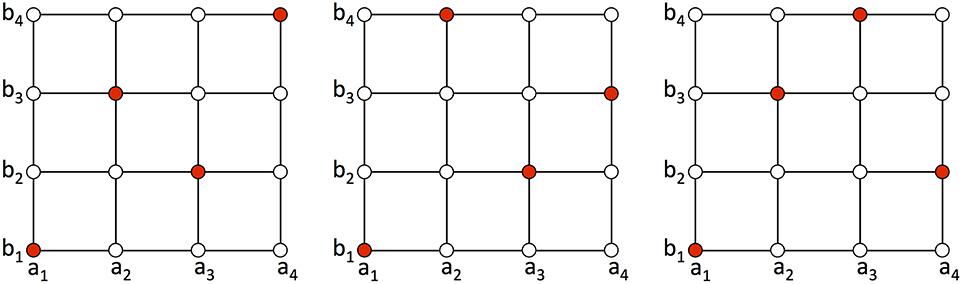
Figure 1. Example of three designs generated via latin hypercube sampling (LHS) in 2D (red points). Note that each of these designs only possesses one point per column and per row, which is a special feature of LHS.

An RBF is a real-valued function that only depends on the Euclidean distance to a center whose location can be set arbitrarily. RBFs provide a class of functions that possess particularly interesting properties such as continuity, smoothness, and infinite differentiability. Their use is widely spread in various branches of applied mathematics and computer science including, e.g., function approximation (Powell, 1993; Buhmann, 2003), data mining and interpolation (Harder and Desmarais, 1972; Lam, 1983; Nychka et al., 2015), numerical analysis with meshfree methods for, e.g., solving partial differential equations in numerical simulations (Fasshauer, 2007; Flyer and Fornberg, 2011; Fornberg and Flyer, 2015; Flyer et al., 2016), computer graphics and machine learning (Broomhead and Lowe, 1988; Boser et al., 1992). Polyharmonic Splines (PHS) are a type of infinitely smooth RBFs that does not possess any free parameter requiring a manual tuning. PHS can therefore be easily implemented for automated calculations.

As previously stated, the goal behind combining sparse calculations of a log-likehood with an RBF decomposition is to limit the number of model evaluations / forward calculations (n) to reduce the computational cost while maintaining a good accuracy on retrieving the exact maximum likelihood. Through low number of model evaluations, we mean to keep n ≲ 100 − 300 regardless of the dimension of the parameter space, such that all model evaluations can easily be performed at once in parallel on a high-performance computing cluster. This provides us with a significant advantage as compared with more traditional sequential optimization methods since the effective computational time of our optimization method would only correspond to the computational time of one model evaluation (because steps 4 and 5 of the method only take up to ≲ 30 s as long as n ≲ 500). The optimization method we propose would, in general, also be more advantageous than a full grid search. Indeed, an accurate full grid search would typically require to sample each parameter of the d-space with about 50−100 points at the least. This rapidly leads to a number of model evaluations that is not practical even when using parallel computing. Finally, ROAM should be competitive with genetic algorithms. Genetic algorithms applied to small population samples, e.g., ≲ a few 100 points, typically require on the order of hundred generations to converge (e.g., Louis and Rawlins, 1993; Gibson and Charbonneau, 1998, and references therein), while faster convergence would require larger population sets. For ROAM, the equivalent of a population sample is a design of the parameter space and the equivalent of a generation would be an iteration of ROAM on a smaller parameter space region. For a population/design of n-points, ROAM should, in principle, be able to converge toward the solution without the need for iterations and, hence, we estimate would be at least 50–100 times faster than a genetic algorithm with the same population/design. In practice, preliminary tests of an iterative implementation of ROAM, which will be published in a subsequent paper, show robust and accurate convergence of ROAM within a few iterations(typically < 10).

3. Results

In this section, we present a set of test cases performed on a synthetic test bed to validate ROAM (Section 2) prior to any observational application. The set of test cases aims at assessing the performance of our method in different circumstances and defining a framework of application that will make use of its strengths.

3.1. Numerical Setup for the Forward Calculations

Our goal is to use the proposed optimization method for data-constrained modeling of the solar coronal magnetic field using, in particular, coronal polarimetric observations (i.e., the four Stokes parameters, (I, Q, U, V), where Stokes I is the total line intensity, Stokes V is the circular polarization, and Stokes Q and U are the two components of the linear polarization). All our test cases are therefore applied to a 3D model of magnetic fields chosen to represent scenarios typically observed in the solar atmosphere. The considered magnetic model is that of a 3D coronal magnetic flux rope generated from a 3D MHD numerical simulation of the emergence of twisted magnetic fields in the solar corona (Figure 2A; Fan, 2012).

FIGURE 2

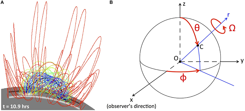
Figure 2. (A) 3D view of the magnetic field of our synthetic test bed. The gray color scale display the photospheric magnetic flux (black/white for negative/positive magnetic flux). The green and blue lines show the magnetic field lines of the twisted flux rope. The red lines correspond to the magnetic field lines of the embedding magnetic field. (B) Schematic of the three parameters considered for our first study. The black thin solid lines highlight the solar photosphere. (θ, ϕ) correspond to the angular coordinates of C, the photospheric center of the 3D box containing the magnetic field of our test bed, while Ω is the rotation angle of that 3D box around the solar radial direction passing by C.

For the test cases, this magnetic field is assumed to depend on four parameters, i.e., height in the corona (h; monotonically depends on the time of the MHD simulation, though not linearly), co-latitude (θ), longitude (ϕ), and rotation angle³ (Ω; of Figure 2B). A series of synthetic polarimetric data, referred to as the ground truth (GT) in the following, is generated for the flux rope associated with $(h;\theta ;\varphi ;\Omega )=(0.16R_{\odot };45^{°};90^{°};30^{°})$ (see Figure 3; note that both Stokes Q and U are presented in a frame of reference relative to the local vertical, or radial coordinate). All synthetic data are computed using the FORWARD Solar Soft IDL package with a field-of-view (FOV) set to $y\times z={\left[0R_{\odot };1.5R_{\odot }\right]}^2$ (where y and z are the POS coordinates) and x = [−0.79; 0.79] R_⊙ for the LOS. We use 192 points along both directions for the POS and 80 points for each LOS, leading to spatial resolutions of 7.6″ and 19.3″ respectively. We limit the forward calculations of the polarization signals to a radial range of [1.03; 1.5] R_⊙, i.e., the FOV of CoMP. Although the spatial resolution of CoMP is 4.5″, we restrict ourselves to a spatial resolution of 7.6″ to allow for relatively fast (about 4–5 min on a MacBook Pro with a 2.7 GHz Intel Core i7 processor) calculations of the polarization signals while maintaining a quasi-CoMP resolution. We impose this FOV and POS spatial resolution to show that CoMP data currently carry meaningful information that can be used to constrain 3D reconstructions of the solar coronal magnetic field.

FIGURE 3

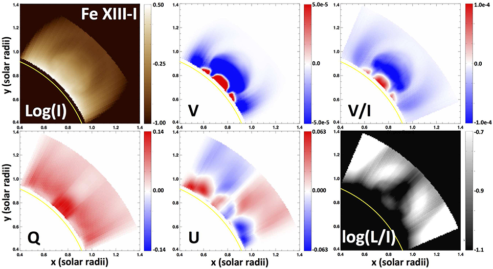
Figure 3. Coronal synthetic images of the polarization signal for the ground truth. All four Stokes parameters (I, Q, U, V) are displayed together with the percentage of circular (V∕I) and linear ($L∕I=\sqrt{(Q^2+U^2)}∕I$) polarization. The yellow solid line shows the solar limb.

Finally, it should be emphasized that the considered flux rope possesses a strong degree of symmetry, such that B (θ; ϕ = 90; Ω ± 180°) = −B (θ; ϕ = 90; Ω). We will exploit these symmetry properties to test ROAM when faced with a log-likelihood function containing multiple maxima.

3.2. Likelihood Function with a Single Maximum

We first apply ROAM in the context of a 3D likelihood function possessing a single maximum. The parameters considered for this study are the co-latitude, longitude, and rotation angle, i.e., (θ; ϕ; Ω). We then build a likelihood function that takes into account all four Stokes parameters, i.e., I, Q, U, and V. For the set {x_i} of a design, we first define the log-likelihood function for a given Stokes parameter, S = {I, Q, U, V}, up to a constant, as

$\begin{array}{cc}{\ell }_S(x_i)=f\left(S(x_i)-S_{gt}\right)=-{\displaystyle \sum _k{\left(S_k(x_i)-S_k^{gt}\right)}^2,}& \left(6\right)\end{array}$

where k is the k-th pixel of the Stokes, S, image. The final log-likelihood function is then constructed as

$\begin{array}{cc}\ell (x_i)=w_I{\ell }_I(x_i)+w_Q{\ell }_Q(x_i)+w_U{\ell }_U(x_i)+w_V{\ell }_V(x_i),& \left(7\right)\end{array}$

where the weighting coefficients w_S were chosen to ensure that I, Q, U, and V similarly contribute to the log-likelihood function, which behavior would otherwise be dominated by the quantity possessing the largest values (here, Stokes I). We use $\left(w_I;w_Q;w_U;w_V\right)=\left(1.3\times 10^{-4};1.9\times 10^{-2};9.2\times 10^{-2};1.2\times 10^4\right)$.

With the log-likelihood function defined in Equation (7), we consider three test cases referred to as 3DN31, 3DN301, and 3DN31ZOOM (see Table 1). These three test cases each contain 100 different designs and differ by the number of points in the designs (31 or 301) as well as by the size of the parameter space to allow us to investigate their role on the performances of ROAM. These test cases are designed to allow us to determine the criteria required for the method to ensure robustness and reliability of the results, i.e., such that the method provides a maximum likelihood estimator (MLE) that gives a good approximation of the parameters of the maximum of the exact likelihood function independently of the design and number of points used.

TABLE 1

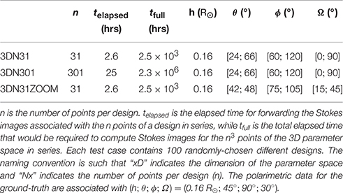
Table 1. Characteristics of the test with a likelihood function possessing a single maximum.

For each test case, the parameters of the RBF decomposition are d = 3, m = 3 and p = m − 1 = 2. We choose the minimum m satisfying the condition 2m − d > 1 (see Section 2). Although θ, ϕ, and Ω all are periodic parameters, their corresponding range is smaller than half the associated period and, hence, no periodic effect is expected. As explained Appendix 2 in Supplementary Material, disregarding the periodicity and curvature of the d-space should not significantly affect the results in such circumstances. We therefore ignore the periodicity of θ, ϕ, and Ω in all 3D cases considered in this section, but return to the issue of periodicity in Section 3.3.

Figure 4 presents 2D dispersion plots of the MLEs obtained for each one of the 100 randomly-chosen designs of the 3DN31 (red), 3DN301 (blue), and 3DN31ZOOM (yellow) cases. For the 3DN31, the MLEs are fairly weakly dispersed for the θ parameter, spanning a range of roughly 10°. As summarized in Table 2, the root mean square (hereafter, rms) of the MLEs, θ_rms, is ≈ 47.1°, which is only ≈ 2.1° different from θ_GT = 45°. This suggests that θ_MLEs is not overly sensitive to the design used for the RBF decomposition. These conclusions contrast with both the ϕ and Ω parameters. Although ϕ_rms ≈ 92.8° is very close to the ground-truth, ϕ_GT = 90°, the ensemble of solutions, ϕ_MLEs, spans the entire ϕ-range considered for the 3DN31. Similarly poor results are obtained for the set of Ω_MLEs, whose rms is ≈ 21° off from the ground-truth, Ω_GT = 30° (see Table 2). Figure 4 further shows that there is a strong coupling between ϕ and Ω. In particular, we find that Ω_MLEs provide a poor estimation of Ω_GT whenever ϕ_MLEs are themselves a poor estimation of ϕ_GT (and vice-versa). Such results trace very poor performances of our optimization method for the chosen setup of the 3DN31 case. The MLE strongly depends on the design used to perform the RBF decomposition. Hence, the MLE obtained from applying our method to a single design is not reliable for the setup of the 3DN31 case.

FIGURE 4

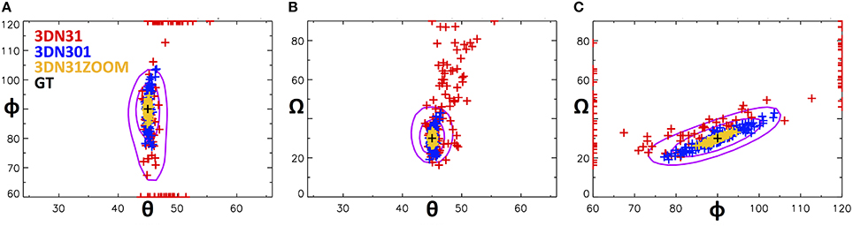
Figure 4. 2D scatter plots of the maximum likelihood estimators (MLEs) found for each design of the 3DN31 (red crosses), 3DN301 (blue crosses), and 3DN31ZOOM (yellow crosses) cases. The black cross highlights the position of the exact maximum (i.e., ground-truth). The two purple solid lines show [0.9; 0.95] × max(ℓ) isocontours. Note that, in panel (B), the red crosses (MLEs of 3DN31) outside the two log-likelihood function isocontours are the solutions associated with ϕ_MLEs = 60° and ϕ_MLEs = 120° from panels (A,C).

TABLE 2

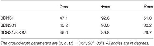
Table 2. Optimization results for a likelihood function with a single maximum.

When comparing 3DN31 to 3DN301 in Figure 4, we can see that increasing the number of points significantly improves the performances of ROAM (see dark blue crosses). For all three parameters, the rms is only ≈ 0.2° off the ground-truth for 3DN301. The range spanned by the ensemble of solutions is relatively smaller than for 3DN31, ≈ 5 times smaller for θ_MLEs and ≈ 3 times smaller for both ϕ_MLEs and Ω_MLEs. Again, the strong coupling between ϕ and Ω is still present but its effect on their uncertainties is strongly reduced as compared with the case 3DN31. Such results are not yet perfect since the set of solutions for both ϕ and Ω is spread over 20°, which is relatively significant considering the range of their values. However, they do show that increasing the number of points per design strongly helps in reducing (a) the dependence of the MLE on the design used for the RBF decomposition, and (b) the effect of (even strong) coupling of parameters on their uncertainty. Increasing the number of points per design therefore strongly helps in improving the reliability and robustness of the proposed optimization method.

Compared with 3DN31, the 3DN31ZOOM case is used to investigate the effect of focusing the parameter space around a region closer to the exact maximum while keeping the number of points per design constant. Figure 4 shows that reducing the size of the parameter space is also beneficial for reducing the MLEs dispersion (see yellow crosses). The rms values for all three parameters are as close to the ground-truth as for 3DN301 (see Table 2) and the solutions are spanning a range that is ≈ 4 times smaller than for 3DN301 and ≈ 12 times smaller than for 3DN31. The MLEs are now independent of the design used for the RBF decomposition for θ and very weakly dependent on that design for both ϕ and Ω. The effect of the strong ϕ − Ω coupling on their uncertainty is again strongly reduced and even smaller than for the 3DN301 case. These very good results prove that ROAM can perform very well and provide an accurate estimation of the ground-truth parameters when the setup is suitably defined.

Figure 5 displays 2D cuts of the exact log-likelihood function and the approximated ones associated with the designs of 3DN31 and 3DN301 giving the best MLEs (referred to as best cases in the following), as well as the approximated log-likelihood function associated with the design of 3DN301 giving the worst MLEs (referred to as worst case). Here, the best (worst) MLE is defined as the MLE minimizing (maximizing) the distance to the ground truth in the parameter space. The best MLE from 3DN31 is (θ; ϕ; Ω)_{best −MLE} = (44.6°; 92.9°; 30.1°) while the best MLE from 3DN301 is (θ; ϕ; Ω)_best−MLE = (45.0°; 89.9°; 30.3°). The worst MLE from 3DN301 is (θ; ϕ; Ω)_best−MLE = (46.5°; 103.7°; 43.0°). The figure shows that the approximated log-likelihood function of the best case from 3DN31 gives an overall rough approximation of the exact one both in terms of values and shape. Note, though, that the rms error on the log-likelihood is 0.24, which is rather small given that max(|ℓ(x)|) ≈ 3.5 for the considered parameter space. For the log-likelihood function of the best case from 3DN301, the results are very much better. The approximated log-likelihood function is able to accurately capture both the values and shape of the exact log-likelihood function; the rms error is 0.05, i.e., ≈ 5 times smaller than for the best case of 3DN31. For the worst case of 3DN301, the rms error on the log-likelihood is 0.25, which is very similar to that of the best case of 3DN31, and the MLE is far from the ground truth for both ϕ and Ω. However, we find that the worst case from 3DN301 provides a more accurate RBF decomposition of the exact log-likelihood function than the best case of 3DN31; the log-likelihood function surfaces display a similar pattern as for the best case of 3DN301 but shifted in the Ω direction. The difference with the 3DN31 lies in the density of points in the entire design, and in the vicinity of the exact maximum, with regard to the structuring, or gradients, of the exact log-likelihood function. This is because the goodness of the approximation is determined by that of the RBF decomposition, which depends on the number of constraints—and hence, points—brought by the design. In other words, the more structured the exact log-likelihood function, the stronger the effect of point density on the goodness of the RBF decomposition / log-likelihood function approximation, similar to what one would expect when discretizing a continuous functions that contains strong gradients. While not shown here, the combined effect of point density and log-likelihood function structuring on the quality of the RBF decomposition is further supported and illustrated by the best case of 3DN31ZOOM that provides the best approximation of the exact log-likelihood function in the vicinity of the exact maximum even though the corresponding design only includes 31 points.

FIGURE 5

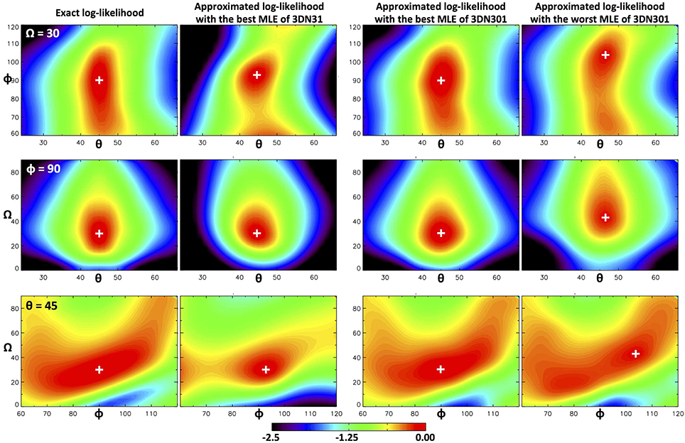
Figure 5. Comparison between approximated and exact log-likelihood functions. The white “+” symbol indicates the position of the maximum log-likelihood.

The aforementioned results show that the RBF decomposition performed well from a sparse sampling of the parameter space, and hence ROAM, is able to capture both the values and variations of the exact log-likelihood function when suitable conditions are met, namely, when the design contains a high enough density of points in the surroundings of the exact maximum and in areas where the exact log-likelihood function is strongly structured. They further demonstrate that ROAM can perform well even with a very low number of points per design although not as robustly. The combined results from 3DN31 and 3DN31ZOOM indicate that an iterative application of ROAM with a smaller and smaller parameter space would be an interesting way to improve its robustness when used with a very sparse design. Such a robust approach has been successfully tested but is beyond the scope of this work and will be presented in a subsequent paper. In particular, the iterative implementation of ROAM strongly improves ϕ_MLEs and Ω_MLEs, leading to a better than 0.5° accuracy on both of these parameters in typically 4–5 iterations with designs of 31 points. The solution is quasi-independent of the design used for the RBF decomposition and the strong ϕ − Ω coupling (previously mentioned and visible in Figure 4C and in the ϕ − Ω cut of the exact log-likelihood function shown in Figure 5) is comfortably reduced and overcome [note that such coupling could also be overcome by separately optimizing one of the coupled parameters, e.g., Ω, and apply ROAM to the 2D parameter space (θ; ϕ)].

Note that, with the goal of increasing speed, and considering our previous comments on the acceptable degree of roughness in the log-likelihood function approximation and an iterative implementation of ROAM, a less sophisticated approach might be conceived. For instance, one could first go through steps 1 to 3 of the method (see Section 2). Then, step 4 (i.e., the RBF decomposition) would be replaced by taking the point of the design associated with the highest log-likelihood function value as a temporary MLE and one would iterate the procedure by defining a smaller design centered around the temporary MLE until a convergence criterion is reached. There are several reasons for not making such a choice. The main reason is that such an initial guess can be far from the exact maximum likelihood, which would likely slow down the convergence by requiring unnecessary iterations and would make the final result more sensitive to local maxima. In addition, applying the RBF decomposition and the search for the maximum from the approximated log-likelihood function is computationally cheap when the number of RBFs is as small as for the cases considered in this study, i.e., typically takes < 10 s for the designs of the 3DN301 case. The benefits of applying steps 4 and 5 of ROAM as proposed in Section 2 (i.e., the RBF decomposition and the search for the MLE from the RBFs approximated log-likelihood function) are illustrated in Figure 6. The figure displays Stokes images for the ground truth, the MLE obtained from fully applying our optimization method to one design of the 3DN301, and for the initial guess from that design. As one can see, the initial MLE guess from the design, (θ; ϕ; Ω)_IG = (46.0°; 101.4°; 45.9°), has a ϕ_IG and Ω_IG that are far off both the ground truth [(θ; ϕ; Ω)_GT = (45.0°; 90.0°; 30.0°)] and the MLE obtained from the RBF decomposition [full application of ROAM; (θ; ϕ; Ω)_MLEs = (44.6°; 90.0°; 28.0°)]. These strong differences in ϕ and Ω result in significantly different Stokes profiles. Iterations would then be needed for the results to be as close to the ground truth as the MLE from the full optimization, which (1) gives a very good estimation of the parameters of the exact maximum likelihood without any real need for iterations, and (2) only takes a few more seconds of calculations.

FIGURE 6

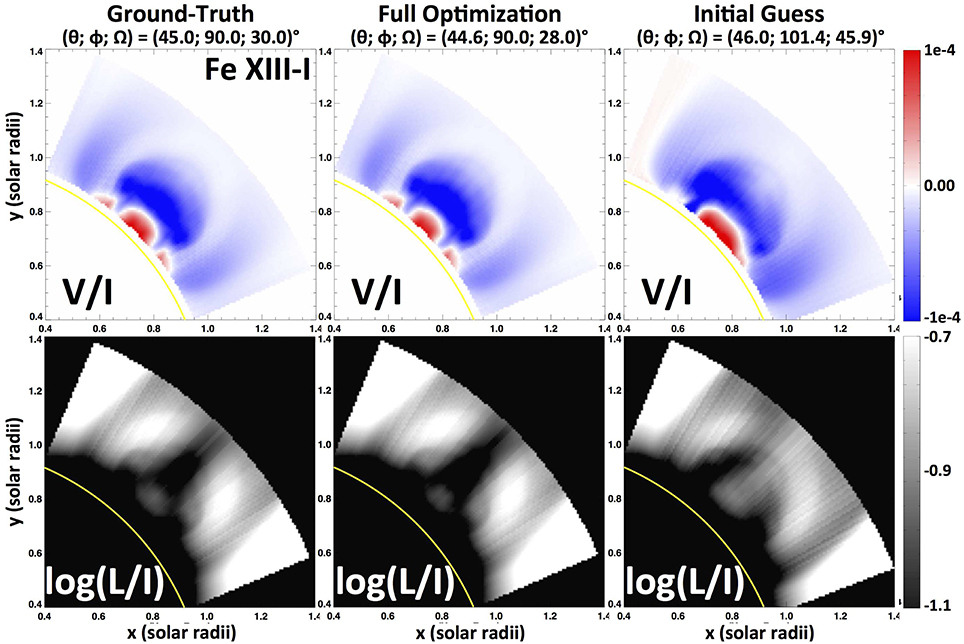
Figure 6. Comparison between polarization signal showing the benefit of steps 4 and 5 of ROAM (see Section 2), for one of the designs of the 3DN301 case. Left column: ground-truth. Middle Column: fully optimized solution (all five steps of the method are applied). Right column: initial guess from the design (i.e., when omitting steps 4 and 5 of ROAM).

In practice, the current capabilities of the CoMP instrument and calibration software do not allow routine measurements of Stokes V since the signal-to-noise ratio is too small. We therefore perform an additional test to show that the current linear polarization signal from CoMP is sufficient to constrain the parameters of a magnetic model using ROAM. The log-likelihood function is defined as in Equation (7) keeping w_I, w_Q, w_U as before, but now setting w_V = 0. The results of that study are displayed in Figure 7 for 3DN301. The figure presents scatter plots of the MLEs of a design obtained when using all four Stokes vs. obtained when using Stokes I, Q, and U only. In such plots, the points should form a line of equation y = x whenever the solutions obtained one way or the other remain the same. As one can see from Figure 7, this is exactly the case for θ_MLEs. Most of the points are also forming a straight line, y = x, for both ϕ_MLEs and Ω_MLEs, with only about 7–8 points (out of 100) being off the line. Such results indicate that a log-likelihood function built from Stokes I, Q, and U contains sufficient information to constrain the three spatial location and orientation parameters considered here. We therefore conclude that the current linear polarization measurements from CoMP contain sufficient observational information to constrain some of the parameters of a given magnetic model.

FIGURE 7

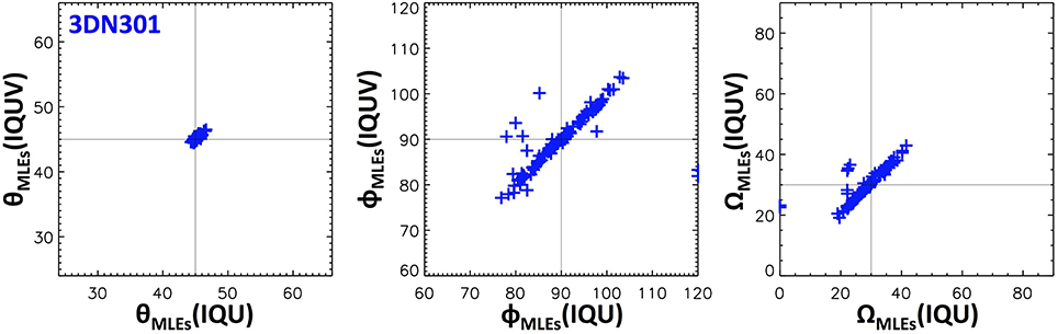
Figure 7. Scatter plots showing the effect of using the circular polarization signal on the MLEs for the 3DN301 case. The thin black solid lines indicate the value of the ground truth.

3.3. Likelihood Function with Multiple Maxima

In this section, we test ROAM in the case of a log-likelihood function with multiple maxima having similar values. For that purpose, we only build the log-likelihood function with Stokes Q and U, setting the weight coefficients of Equation (7) to $(w_I;w_Q,w_U,w_V)=(0.;2.0\times 10^{-2};6.9\times 10^{-2};0.)$. Only the height of the flux rope in the corona, h, and the tilt angle, Ω, are considered for this test (see Table 3 for the range of values considered for each parameter).

TABLE 3

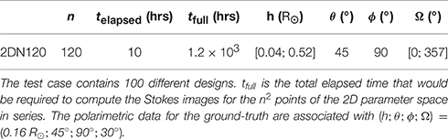
Table 3. Characteristics of the test with a likelihood function possessing multiple maxima.

Stokes Q and U signals are associated with the transverse magnetic field, i.e., the component of a magnetic field perpendicular to the LOS. For a single point in the solar corona, the transverse magnetic field diagnosed from either the Hanle or Zeeman effect is subject to a 180° ambiguity (e.g., Casini and Judge, 1999; Judge, 2007). In terms of the parameters considered in our tests, it means that a single point magnetic field set with a rotation angle, Ω_SP, will give the same Stokes Q and U signals as when set with Ω_SP ± 180°. Considering that ϕ_GT = 90° (that is, the flux rope is centered at the solar limb) and the strong symmetry of our flux rope (see Section 3.1), we expect the LOS integrated Stokes Q and U to be the same for Ω and Ω ± 180°, resulting in a log-likelihood function with two maxima respectively located at Ω_GT and Ω_GT ± 180°; note that the symmetry of Stokes Q and U would be broken if the flux rope were not centered on the solar limb. This is indeed the case as shown Figure 8B where a maximum region can be observed at Ω = 30° and Ω = 210°. Figure 8B further shows the presence of two additional maximum regions located at Ω = 150 and 330°. These two solutions suggest a symmetry with regard to the plane Ω = 0° that is not expected. We find that the corresponding Stokes Q and U images are, as expected, different from those of the ground truth. However, the differences are small as compared with other values of Ω, resulting in a local maximum in those two regions. Note, though, that these four maximum regions are only possible because ϕ = 90°, whereas any other value of ϕ would break the symmetry of the Stokes Q and U images.

FIGURE 8

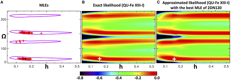
Figure 8. Likelihood function with multiple maxima. (A) Scatter plots of the maximum likelihood estimators (MLEs) found for each design of the 2DN120 (red crosses) case. (B) Surface plot of the exact log-likelihood function possessing 2 global (Ω = {30;210}°) and 2 local (Ω = {150;330}°) maxima. (C) Approximated log-likelihood function with the best MLE of 2DN120. The white and black crosses highlight the position of the exact maximum (i.e., ground-truth). The purple solid lines show 0.95 × max(ℓ) isocontours.

In the present test case, the periodic parameter Ω varies on a range of values larger than half its period. In such circumstances, we must consider its periodicity for the RBF decomposition (see Appendix 2 in Supplementary Material). Accordingly, the parameters of the RBF decomposition are d′ = 3, m = 3 and p = m − 1 = 2. As in Section 3.2, we run our optimization method on 100 different designs whose properties are given in Table 3. The results are summarized in a 2D dispersion plot in Figure 8A. The figure shows that the 100 MLEs are mainly, and almost equally, clustering around the two global Ω maximum regions, corresponding to the ground truth and its counterpart at 180°. We further find that, out of these 100 solutions, only four are associated with one of the two local maximum regions, here Ω ≈ 150°. As for the height of the MLEs, we find an average value of $1.6\times 10^{-1}{R}_{\odot }$ with a 2σ dispersion level of $0.5\times 10^{-1}{R}_{\odot }$, meaning that the height is well constrained even from using Stokes Q and U only. The dispersion plot from Figure 8A therefore indicates that our optimization method is strongly sensitive to multiple global maxima and can be sensitive to local maxima. Note that the sensitivity to local maxima depends upon both the number of points used in the design and the value of these local maxima relatively to that of the global maxima.

Figure 8C displays a surface plot of the log-likelihood function from the best case of 2DN120. As one can see, the RBF decomposition is able to capture both the values and shapes of the exact log-likelihood function. We find an rms error of 0.04 on the log-likelihood. The RBF decomposition can therefore provide a good approximation of the exact log-likelihood function even with a periodic space and the presence of multiple maxima.

Finally, we show in Figure 9 that using the Stokes V signal to build the log-likelihood function removes the Ω ambiguities that were observed in the log-likelihood function constructed from Stokes Q and U only. When using Stokes V, the optimization leads to Ω_rms ≈ 28.8°. This means that some additional observables might be worth considering to remove ambiguities in parameters when they exist. Another alternative to remove ambiguities is to reduce the parameter space to regions having a single maximum. Then, one can either study each region separately or use prior constraints to eliminate regions that are very unlikely. For instance, one can use the photospheric magnetograms, or Hα observations, prior to or after the passage of the flux rope at a limb to estimate the rotation angle (i.e., Ω) and put strong constraints on the values of rotation angle to consider for the parameter space.

FIGURE 9

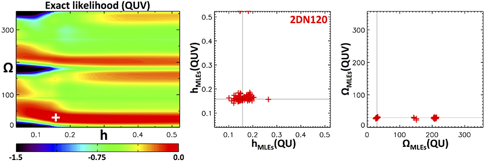
Figure 9. Effect of using circular polarization on the log-likelihood function of Figure 8B.

3.4. Stability with Regard to Noise in the Data

In practice, any real data is subject to measurement errors. Such errors may prevent the retrieval of any meaningful information about the polarization, and hence, the magnetic field in regions of weak signals and/or when the signal-to-noise ratio is weak. The results of ROAM might be sensitive to such noise and we therefore need to investigate that sensitivity. For that reason, we now test our method when the synthetic observations associated with the ground truth contain some noise. In this regard, we build the log-likelihood function with Stokes U images only

$\begin{array}{cc}\ell (x_i)=\frac{{\ell }_U(x_i)}{{\sigma }_U^2},& \left(8\right)\end{array}$

where σ_U is the root mean square of the noise in the synthetic Stokes U signal of the ground truth.

For a given value of photon noise, σ_I, σ_Q, σ_U, σ_V are all different. As a consequence, if one uses more than one Stokes component, then varying the noise further changes the relative contribution of each Stokes parameter to the log-likelihood function due to the weighting by 1∕σ_S. We need to be free of the variation of relative contribution of the different Stokes in order to isolate the sole effect of noise on the robustness of our optimization method, which then implies using only one Stokes parameter to define the log-likelihood function. Considering CoMP capabilities and the current magnetic model and ground truth, we performed several tests with different levels of noise (which can be added using FORWARD) and found that (1) Stokes V cannot be used for realistic exposure times because its values for our test bed are too weak and would require an unrealistic 4 days exposure time to reach a moderate level of noise for the particular choices of ground-truth parameters and pixel sizes (see corresponding values in Section 3.1), (2) Stokes I cannot be used because it is not sensitive enough to noise (even a 1 s exposure time leads to a very weak level of noise), and (3) Stokes Q and U are better suited for the noise test with exposure times of the order of 1–100 s. From this analysis, we chose Stokes U because it was slightly more sensitive to noise than Stokes Q for the setup considered in this paper (note that both Q and U are presented in a frame of reference relative to the local vertical, or radial coordinate).

FORWARD already implements a photon noise calculation for the infra-red lines under consideration (see e.g., Gibson et al., 2016). The noise is calculated according to the specifications of the instrument considered (telescope aperture, detector efficiency), the background photon level, and the exposure time to obtain a forward calculation that includes the noise. For CoMP, the aperture is 20 cm, the efficiency is 0.05 throughput and the background is five parts per million of solar brightness. We perform three tests with different exposure time, t_exp, hence noise level, i.e., t_exp = (1; 10; 300) seconds that respectively correspond to strong, moderate, and weak noise cases for the considered setup. The synthetic Stokes U images of the ground truth for these noise levels are displayed in Figure 10. These synthetic ground truth are used with all designs of the 3DN31, 3DN301, and 3DN31ZOOM cases.

FIGURE 10

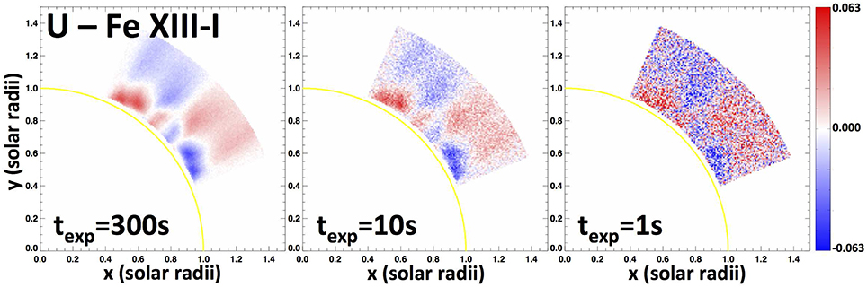
Figure 10. Synthetic Stokes U images of the ground truth for different exposure times, t_exp, and hence, noise levels.

Figure 11 presents scatter plots of the error on the MLEs obtained when noise is included in the ground truth Stokes U images as compared with the case when no noise is considered. The plots are only shown for the Ω parameter because all three parameters θ, ϕ, and Ω display very similar results. In Figure 11, one can see a nearly perfect horizontal line at y = 0 for Ω_MLEs obtained with an exposure time of 300 s (yellow crosses) for all test cases (3DN31, 3DN301, and 3DN31ZOOM). This means that the t_exp = 300 s case is equivalent to the no-noise case. For cases t_exp = 10 and t_exp = 1 s, the plots show some departure from the y = 0 line, which increases with the level of noise. The figure also shows that the noise effect on the robustness of the MLEs depends on the density of points in the designs, i.e., 3DN31 is the most affected by the noise while 3DN31ZOOM is the least affected. That being said, we find that only less than ≈ 10 − 15 points (out of 100) of 3DN31 exhibit a strong sensitivity to noise for the t_exp = 1 second case, i.e., with an error >5°. This number drops to ≈ 5 when t_exp = 10 s. For the t_exp = 1 s, Figure 10 shows that the noise strongly masks the real Stokes U signal, although not entirely. We therefore deduce that our optimization method is very stable against the presence of noise in the data as long as the noise does not entirely mask the real signal. Considering that Stokes Q is similarly sensitive to noise as Stokes U and that Stokes I is much less sensitive to the noise, we conclude that our method can be robustly used with the Stokes I, Q, and U data provided by the CoMP.

FIGURE 11

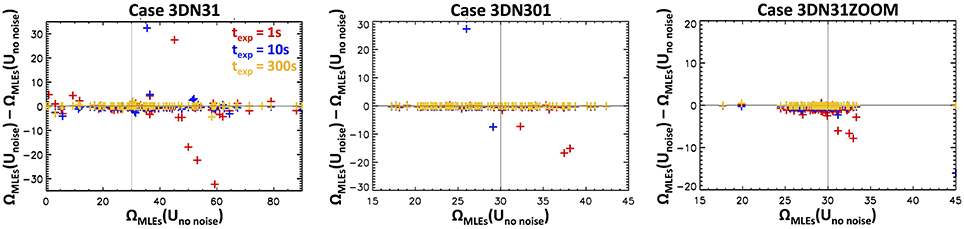
Figure 11. Scatter plots showing the effect of noise on the MLEs obtained with ROAM for all designs of 3DN31, 3DN301, and 3DN31ZOOM. The horizontal, thin black line indicates the zero error level, while the vertical thin black line indicates the ground-truth value.

4. Conclusions

In this paper, we introduced and validated a new optimization method for model-data fitting, ROAM (Radial-basis-functions Optimization Approximation Method). Our primary motivation for this work has been to develop a novel approach for diagnosing the solar coronal magnetic field by combining a parameterized 3D magnetic field model with forward modeling of coronal polarization. From various tests applied to the synthetic test bed of a coronal magnetic flux rope, we showed that ROAM allows for fast, efficient, and accurate model-data fitting in a d-dimensional parameter space. These test cases further enabled us to analyze and specify a framework for an optimal application of ROAM.

Applying our method with forward modeling of IR coronal polarimetry, we demonstrated that ROAM can be exploited for converting coronal polarimetric measurements into magnetic field data. The use of our model-data fitting method therefore opens new perspectives for the development and exploitation of coronal polarimetric measurements such as the ones routinely performed by CoMP (Tomczyk et al., 2008) and future telescopes such as the Daniel K. Inoue Solar Telescope⁴ and the Coronal Solar Magnetism Observatory (Tomczyk et al., 2016), but also for a wider range of coronal observations including, e.g., UV (see e.g., Fineschi, 2001; Raouafi et al., 2009) and radio polarimetry (e.g., White and Kundu, 1997; Gelfreikh, 2004; see also Gibson et al., 2016, for discussion of multiwavelength magnetometry).

Beyond the analysis of coronal polarimetric measurements, ROAM offers interesting perspectives for magnetic field reconstruction models. Most of the current 3D diagnostics of the coronal magnetic field of solar active regions (ARs) are derived from the analysis of magnetic field reconstruction models including, e.g., force-free field extrapolations of the photospheric magnetic field (see e.g., Alissandrakis, 1981; Demoulin et al., 1989; Wheatland et al., 2000; Yan and Sakurai, 2000; Wiegelmann, 2004; Amari et al., 2006; Malanushenko et al., 2012, and references therein), and magneto-frictional methods (see e.g., van Ballegooijen, 2004; Valori et al., 2005, 2007; Jiang et al., 2011; Inoue et al., 2012; Titov et al., 2014, and references therein). ROAM could, in principle, be used to perform model-data fitting with such reconstruction models that either already are (i.e., through the poloidal and axial flux for the magneto-frictional methods with flux rope insertion) or could be (e.g., through the photospheric force-free parameter for both force-free field extrapolations and magneto-frictional methods without flux rope insertion) parameterized. The extensive work performed over the years in terms of forward modeling of various observables (see e.g., Gibson et al., 2016, and references therein) would then allow for using several types of different observations to constrain the parameters of the magnetic field reconstruction models. ROAM therefore opens new perspectives for including coronal polarimetric measurements into magnetic field reconstructions and, more generally, for data-optimized reconstruction of the solar coronal magnetic field. Such perspectives will be tackled in the framework of the Data Optimized Coronal Field Model⁵ (DOCFM), a collaborative project that will make use of ROAM.

Finally, we wish to mention that ROAM is not limited to coronal magnetic field diagnostics and could be used for other optimization problems. The method will be of particular interest for model-data fitting for which a model evaluation (here, the evaluation of the model itself and/or the forward modeling of an observable if applicable) is computationally expensive.

Author Contributions

All authors listed, have made substantial, direct and intellectual contribution to the work, and approved it for publication.

Funding

KD acknowledges funding from the Computational and Information Systems Laboratory and from the High Altitude Observatory, and along with SG and YF acknowledges support from the Air Force Office of Scientific Research under award FA9550-15-1-0030.

Conflict of Interest Statement

The authors declare that the research was conducted in the absence of any commercial or financial relationships that could be construed as a potential conflict of interest.

Acknowledgments

We thank the two anonymous referees and Anna Malanushenko for a careful consideration of the manuscript and constructive comments. The National Center for Atmospheric Research is sponsored by the National Science Foundation.

Supplementary Material

The Supplementary Material for this article can be found online at: https://www.frontiersin.org/article/10.3389/fspas.2016.00024

Footnotes

1. ^http://www.hao.ucar.edu/FORWARD/

2. ^http://www.lmsal.com/solarsoft/

3. ^Note that (θ; ϕ; Ω) are the co-latitude, longitude, and rotation angle of the numerical box—containing the magnetic field of the MHD simulation—around the Sun, while h is the actual height of the flux rope in that numerical box (inside of which the solar photosphere is located at h = 0).

4. ^http://www.ifa.hawaii.edu/~schad/dlnirsp/

5. ^http://www.hao.ucar.edu/DOCFM/

References

Alissandrakis, C. E. (1981). On the computation of constant alpha force-free magnetic field. Astron. Astrophys. 100, 197–200.

Google Scholar

Amari, T., Boulmezaoud, T. Z., and Aly, J. J. (2006). Well posed reconstruction of the solar coronal magnetic field. Astron. Astrophys. 446, 691–705. doi: 10.1051/0004-6361:20054076

CrossRef Full Text | Google Scholar

Bird, M. K., Volland, H., Howard, R. A., Koomen, M. J., Michels, D. J., Sheeley, N. R. Jr., et al. (1985). White-light and radio sounding observations of coronal transients. Solar Phys. 98, 341–368. doi: 10.1007/BF00152465

CrossRef Full Text | Google Scholar

Bommier, V., and Sahal-Brechot, S. (1982). The Hanle effect of the coronal L-alpha line of hydrogen - Theoretical investigation. Solar Phys. 78, 157–178. doi: 10.1007/BF00151151

CrossRef Full Text

Boser, B. E., Guyon, I. M., and Vapnik, V. N. (1992). “A training algorithm for optimal margin classifiers,” in Proceedings of the Fifth Annual Workshop on Computational Learning Theory, COLT '92, (New York, NY: ACM), 144–152. doi: 10.1145/130385.130401

CrossRef Full Text | Google Scholar

Broomhead, D. S. Lowe, D. (1988). Multivariable functional interpolation and adaptive networks. Complex Syst. 2, 321–355.

Google Scholar

Buhmann, M. D. (2003). Radial Basis Functions: Theory and Implementations. Cambridge, UK: Cambridge Monographs on Applied and Computational Mathematics; Cambridge University Press.

Google Scholar

Casini, R., and Judge, P. G. (1999). Spectral lines for polarization measurements of the coronal magnetic field. II. Consistent treatment of the stokes vector for magnetic-dipole transitions. Astrophys. J. 522, 524–539. doi: 10.1086/307629

CrossRef Full Text | Google Scholar

Demoulin, P., Priest, E. R., and Anzer, U. (1989). A three-dimensional model for solar prominences. Astron. Astrophys. 221, 326–337.

Google Scholar

Duchon, J. (1977). Constructive Theory of Functions of Several Variables: Proceedings of a Conference Held at Oberwolfach April 25 – May 1, 1976. Berlin; Heidelberg: Springer Berlin Heidelberg. doi: 10.1007/BFb0086566

CrossRef Full Text | Google Scholar

Fan, Y. (2012). Thermal signatures of tether-cutting reconnections in pre-eruption coronal flux ropes: hot central voids in coronal cavities. Astrophys. J. 758:60. doi: 10.1088/0004-637X/758/1/60

CrossRef Full Text | Google Scholar

Fasshauer, G. E. (2007). Meshfree Approximation Methods with MATLAB, Vol. 6 of Interdisciplinary Mathematical Sciences. Singapore: World Scientific Publishing Company.

Google Scholar

Fineschi, S. (2001). “Space-based instrumentation for magnetic field studies of solar and stellar atmospheres,” in Magnetic Fields Across the Hertzsprung-Russell Diagram, Vol. 248 of Astronomical Society of the Pacific Conference Series, eds G. Mathys, S. K. Solanki, and D. T. Wickramasinghe (San Francisco, CA: Astronomical Society of the Pacific), 597.

Flyer, N., Barnett, G. A., and Wicker, L. J. (2016). Enhancing finite differences with radial basis functions: experiments on the Navier-Stokes equations. J. Comput. Phys. 316, 39–62. doi: 10.1016/j.jcp.2016.02.078

CrossRef Full Text | Google Scholar

Flyer, N., and Fornberg, B. (2011). Radial basis functions: developments and applications to planetary scale flows. Comput. Fluids 46, 32. doi: 10.1016/j.compfluid.2010.08.005

CrossRef Full Text | Google Scholar

Fornberg, B. Flyer, N. (2015). Solving PDEs with radial basis functions. Acta Numerica 24, 215–258. doi: 10.1017/S0962492914000130

CrossRef Full Text | Google Scholar

Gelfreikh, G. B. (2004). “Coronal magnetic field measurements through Bremsstrahlung emission,” in Astrophysics and Space Science Library, Vol. 314 of Astrophysics and Space Science Library, eds D. E. Gary and C. U. Keller (Dordrecht: Springer), 115. doi: 10.1007/1-4020-2814-86

CrossRef Full Text

Gibson, S., Kucera, T., White, S. M., Dove, J., Fan, Y., Forland, B., et al. (2016). FORWARD: a toolsel for multiwavelength coronal magnetometry. Front. Astron. Space Sci. 3:8. doi: 10.3389/fspas.2016.00008

CrossRef Full Text | Google Scholar

Gibson, S. E., and Charbonneau, P. (1998). Empirical modeling of the solar corona using genetic algorithms. J. Geophys. Res. 103, 14511–14522. doi: 10.1029/98JA00676

CrossRef Full Text | Google Scholar

Hale, G. E. (1908). On the probable existence of a magnetic field in sun-spots. Astrophys. J. 28, 315. doi: 10.1086/141602

CrossRef Full Text | Google Scholar

Hanle, W. (1924). Über magnetische Beeinflussung der Polarisation der Resonanzfluoreszenz. Z. Phys. 30, 93–105. doi: 10.1007/BF01331827

CrossRef Full Text | Google Scholar

Harder, R. L., and Desmarais, R. N. (1972). Interpolation using surface splines. J. Aircraft 9, 189–191. doi: 10.2514/3.44330

CrossRef Full Text | Google Scholar

Iman, R. L., Helton, J. C., and Campbell, J. E. (1981). An approach to sensitivity analysis of computer models, part 1. introduction, input variable selection and preliminary variable assessment. J. Qual. Technol. 13, 174–183.

Google Scholar

Inoue, S., Magara, T., Watari, S., and Choe, G. S. (2012). Nonlinear force-free modeling of a three-dimensional sigmoid observed on the sun. Astrophys. J. 747:65. doi: 10.1088/0004-637X/747/1/65

CrossRef Full Text | Google Scholar

Jiang, C., Feng, X., Fan, Y., and Xiang, C. (2011). Reconstruction of the coronal magnetic field using the CESE-MHD Method. Astrophys. J. 727:101. doi: 10.1088/0004-637X/727/2/101

CrossRef Full Text | Google Scholar

Jones, D. R., Schonlau, M., and Welch, W. J. (1998). Efficient global optimization of expensive black-box functions. J. Glob. Optimization 13, 455–492. doi: 10.1023/A:1008306431147

CrossRef Full Text | Google Scholar

Judge, P. G. (2007). Spectral lines for polarization measurements of the coronal magnetic field. V. Information content of magnetic dipole lines. Astrophys. J. 662, 677–690. doi: 10.1086/515433

CrossRef Full Text | Google Scholar

Judge, P. G., Low, B. C., and Casini, R. (2006). Spectral lines for polarization measurements of the coronal magnetic field. IV. Stokes signals in current-carrying fields. Astrophys. J. 651, 1229–1237. doi: 10.1086/507982

CrossRef Full Text | Google Scholar

Kramar, M., Airapetian, V., Mikić, Z., and Davila, J. (2014). 3D coronal density reconstruction and retrieving the magnetic field structure during solar minimum. Solar Phys. 289, 2927–2944. doi: 10.1007/s11207-014-0525-7

CrossRef Full Text | Google Scholar

Lam, N. S. N. (1983). Spatial interpolation methods: a review. Am. Cartogr. 10, 129–149.

Google Scholar

Lin, H., Kuhn, J. R., and Coulter, R. (2004). Coronal magnetic field measurements. Astrophys. J. 613, L177–L180. doi: 10.1086/425217

CrossRef Full Text | Google Scholar

López Ariste, A. (2015). “Magnetometry of prominences,” in Solar Prominences, Vol. 415 of Astrophysics and Space Science Library, eds J.-C. Vial and O. Engvold (Cham: Springer International Publishing), 179.

Louis, S. J., and Rawlins, G. J. E. (1993). “Syntactic analysis of convergence in genetic algorithms,” in Foundations of Genetic Algorithms - 2, ed L. D. Whitley (San Mateo, CA: Morgan Kauffman), 141–152.

Google Scholar

Madych, W. R., and Nelson, S. A. (1990). Polyharmonic cardinal splines. J. Approx. Theory 60, 141–156. doi: 10.1016/0021-9045(90)90079-6

CrossRef Full Text | Google Scholar

Malanushenko, A., Schrijver, C. J., DeRosa, M. L., Wheatland, M. S., and Gilchrist, S. A. (2012). Guiding nonlinear force-free modeling using coronal observations: first results using a Quasi-Grad-Rubin scheme. Astrophys. J. 756:153. doi: 10.1088/0004-637X/756/2/153

CrossRef Full Text | Google Scholar

McKay, M. D., Beckman, R. J., and Conover, W. J. (1979). A comparison of three methods for selecting values of input variables in the analysis of output from a computer code. Technometrics 21, 239–245.

Nychka, D., Bandyopadhyay, S., Hammerling, D., Lindgren, F., and Sain, S. (2015). A multiresolution gaussian process model for the analysis of large spatial datasets. J. Comput. Graphical Stat. 24, 579–599. doi: 10.1080/10618600.2014.914946

CrossRef Full Text | Google Scholar

Plowman, J. (2014). Single-point inversion of the coronal magnetic field. Astrophys. J. 792:23. doi: 10.1088/0004-637X/792/1/23

CrossRef Full Text | Google Scholar

Powell, M. J. D. (1977). Restart procedures for the conjugate gradient method. Math. Programming 12, 241–254. doi: 10.1007/BF01593790

CrossRef Full Text | Google Scholar

Powell, M. J. D. (1993). Some Algorithms for Thin Plate Spline Interpolation to Functions of Two Variables. Cambridge University Dept. of Applied Mathematics and Theoretical Physics technical report.

Rachmeler, L. A., Casini, R., and Gibson, S. E. (2012). “Interpreting Coronal Polarization Observations,” in Second ATST-EAST Meeting: Magnetic Fields from the Photosphere to the Corona., Vol. 463 of Astronomical Society of the Pacific Conference Series, eds T. R. Rimmele, A. Tritschler, F. Wöger, M. Collados Vera, H. Socas-Navarro, R. Schlichenmaier, M. Carlsson, T. Berger, A. Cadavid, P. R. Gilbert, P. R. Goode, and M. Knölker (San Francisco, CA: Astronomical Society of the Pacific), 227.

Rachmeler, L. A., Gibson, S. E., Dove, J. B., DeVore, C. R., and Fan, Y. (2013). Polarimetric properties of flux ropes and sheared arcades in coronal prominence cavities. Solar Phys. 288, 617–636. doi: 10.1007/s11207-013-0325-5

CrossRef Full Text | Google Scholar

Raouafi, N.-E., Solanki, S. K., and Wiegelmann, T. (2009). “Hanle effect diagnostics of the coronal magnetic field: a test using realistic magnetic field configurations,” in Solar Polarization 5: In Honor of Jan Stenflo, Vol. 405 of Astronomical Society of the Pacific Conference Series, eds S. V. Berdyugina, K. N. Nagendra, and R. Ramelli (San Francisco, CA: Astronomical Society of the Pacific), 429.

Sahal-Brechot, S., Bommier, V., and Leroy, J. L. (1977). The Hanle effect and the determination of magnetic fields in solar prominences. Astron. Astrophys. 59, 223–231.

Google Scholar

Stenflo, J. O. (2015). History of solar magnetic fields since George Ellery Hale. Space Sci. Rev. 1–31. doi: 10.1007/s11214-015-0198-z

CrossRef Full Text | Google Scholar

Titov, V. S., Török, T., Mikic, Z., and Linker, J. A. (2014). A method for embedding circular force-free flux ropes in potential magnetic fields. Astrophys. J. 790:163. doi: 10.1088/0004-637X/790/2/163

CrossRef Full Text | Google Scholar

Tomczyk, S., Card, G. L., Darnell, T., Elmore, D. F., Lull, R., Nelson, P. G., et al. (2008). An instrument to measure coronal emission line polarization. Solar Phys. 247, 411–428.

Google Scholar

Tomczyk, S., Landi, E., Burkepile, J. T., Casini, R., DeLuca, E. E., Fan, Y., et al. (2016). Scientific objectives and capabilities of the Coronal Solar Magnetism Observatory. J. Geophys. Res. Space Phys. doi: 10.1002/2016JA022871

CrossRef Full Text | Google Scholar

Valori, G., Kliem, B., and Fuhrmann, M. (2007). Magnetofrictional extrapolations of low and lou's force-free equilibria. Solar Phys. 245, 263–285. doi: 10.1007/s11207-007-9046-y

CrossRef Full Text | Google Scholar

Valori, G., Kliem, B., and Keppens, R. (2005). Extrapolation of a nonlinear force-free field containing a highly twisted magnetic loop. Astron. Astrophys. 433, 335–347. doi: 10.1051/0004-6361:20042008

CrossRef Full Text | Google Scholar

van Ballegooijen, A. A. (2004). Observations and modeling of a filament on the Sun. Astron. Astrophys. 612, 519–529. doi: 10.1086/422512

CrossRef Full Text | Google Scholar

Wheatland, M. S., Sturrock, P. A., and Roumeliotis, G. (2000). An optimization approach to reconstructing force-free fields. Astron. Astrophys. 540, 1150–1155. doi: 10.1086/309355

CrossRef Full Text | Google Scholar

White, S. M., and Kundu, M. R. (1997). Radio observations of gyroresonance emission from coronal magnetic fields. Solar Phys. 174, 31–52. doi: 10.1023/A:1004975528106

CrossRef Full Text | Google Scholar

Wiegelmann, T. (2004). Optimization code with weighting function for the reconstruction of coronal magnetic fields. Solar Phys. 219, 87–108.

Google Scholar

Yan, Y. Sakurai, T. (2000). New boundary integral equation representation for finite energy force-free magnetic fields in open space above the Sun. Solar Phys. 195, 89–109. doi: 10.1023/A:1005248128673

CrossRef Full Text | Google Scholar