Self-Gravitating Stellar Collapse: Explicit Geodesics and Path Integration

1. Introduction

Black holes play a pivotal role in the evolution of the universe providing an important test laboratory for general relativity. Within classical general relativity, Oppenheimer and Synder modeled the gravitational collapse of star to a black hole by approximating the star with a uniform sphere of dust (hereafter O-S model) (Oppenheimer and Snyder, 1939). This model provides an analytic solution for stellar collapse that connects the Schwarzschild exterior of a star to a contracting Friedmann-Robertson-Walker (FRW) interior. Once the surface has passed within r = 2M, no internal pressures can halt the collapse and all configurations collapse to a point-like singularity at r = 0. The general features of this toy collapse model have been examined by many authors (Vaidya, 1951; Misner et al., 1973; Singh and Witten, 1997; Goswami and Joshi, 2004; Joshi, 2007).

In the standard formalism from Misner et al. (1973), the stellar surface is considered to be initially at rest. Here we consider configurations with all possible initial velocities. We derive closed-form solutions for the equations of motion in Schwarzschild and Kruskal coordinates for space-like, time-like, and light-like geodesics.

As an example application of our closed-form solutions for the classical O-S model with non-zero initial velocities, we consider the macroscopic collapse of a spherically symmetric sphere of dust composed of ultra-light particles. To approximate quantum effects, the radius of the star is approximated by a Gaussian wavepacket that is initially centered far from r = 2M. Its evolution is then followed via a simple path integral approach that extends the results of Redmount and Suen (1993) from a relativistic free particle to a particle constrained by non-trivial gravity. Gravitational collapse incorporating approximate treatments of quantum mechanics has been considered by a variety of authors (Hájíček et al., 1992; Hawkins, 1994; Casadio and Venturi, 1996; Ansoldi et al., 1997; Berezin, 1997; Zloshchastiev, 1998; Alberghi et al., 1999; Vaz and Witten, 2001; Corichi et al., 2002; Ortíz and Ryan, 2007). They involve non-equivalent ways of quantization that often produce physically different results (Dolgov and Khriplovich, 1997). Our path-integral approach approach is simpler, and can be easily compared to the assumption that the particle obeys the relativistic Schrödinger equation.

In the classical model a star is idealized as a collapsing self-gravitating dust sphere of uniform density and zero pressure where the constituent particles have the attributes of classical dust: each particle is assumed to be infinitesimal in size and to interact only gravitationally with other matter. The inclusion of quantum mechanical effects lifts some of these assumptions allowing for the possibility that some configurations will not collapse to black holes but will disperse or even form stable new configurations. Quantitatively, quantum treatment is necessary in macroscopic stellar collapse when the action S is of the order ℏ (Narlikar, 1977). In our case, the S/ℏ ~ 1 condition corresponds to mM ~ ℏ. For macroscopic black holes of masses $M=1M_{\odot }-10^9{M}_{\odot }$, this implies that quantum treatment is necessary for ultra-light constituent particles of m ~ 10⁻¹⁰ − 10⁻¹⁹ eV. In nature, such ultralight particle could be dark matter. Dark matter comes close to the attributes of classical dust, and some dark matter clouds may be dense enough to collapse to black holes. Particles as light as 10⁻²² − 10⁻²³ eV have been proposed as constituents of dark matter halos (Hu et al., 2000; Lesgourgues et al., 2002; Lundgren et al., 2010; Khmelnitsky and Rubakov, 2014).

To approximate quantum effects of the collapse of such a halo comprised of ultra-light particles, we start with an initial wavefunction that represents the position of the particle on the stellar surface, and is at first far from 2M. To study the propagation of the wavefunction, we integrate over all possible paths taken by the particle. At a given time, the outgoing wavefunction comprises the probability that the star disperses, and the ingoing wavefunction the probability that it collapses. We compute the propagator in analytical form for a particle on the surface of the star in the WKB approximation, and compare this to the limited assumption that the particle obeys the relativistic Schrödinger equation. Our equations reduce to a free particle case when the mass of the star is zero; then the solution to the relativistic Schrödinger equation is the exact representation of the wave function (Redmount and Suen, 1993). In the more general case of a particle on the surface of a star, this representation is no longer correct. However, the comparison is instructive. As expected, we observed that the WKB and relativistic Schrödinger approximations are out of step at early and late times, and appear to converge toward one another at intermediate times.

In Schwarzschild coordinates, we can follow the evolution of the surface of the star only until the formation of an apparent horizon due to the r = 2M coordinate singularity. In Kruskal coordinates, one can continue to study the evolution of the star inside the apparent horizon (r < 2M). The paths we have derived here include time-reversing space-like paths, which allow for the possibility of extraction of information from inside the horizon to the outside. These paths turn inside the horizon r > 0, and head toward r = 2M. In future work, explicit geodesic equations in Kruskal coordinates may be used as a stepping stone to model behavior inside r = 2M.

The rest of the paper is structured as follows: in Section 2 we describe the Oppenheimer–Snyder model. Section 3 includes an overview of the classical action and paths, a computation of the Oppenheimer–Snyder limit and the derivation of the classical paths in Schwarzschild coordinates. Section 4 details the classical paths in Kruskal coordinates, which comprise a starting point for future work that explores the collapse inside r = 2M. As an example application of the closed form geodesics, Section 5 describes the quantum treatment of the dust collapse applicable to ultra-light particles in Schwarzschild coordinates. The conclusions follow in Section 6.

2. The Oppenheimer–Snyder Model

In General Relativity, a first approximation to the exterior space-time of any star, planet or black hole is a spherically symmetric space-time modeled by the Schwarzschild metric. This is a consequence of Birkhoff's theorem (Misner et al., 1973). The Schwarzschild line element thus takes the usual form

$\begin{array}{ll}d{s}^2=-\left(1-\frac{2M}{r}\right)d{t}^2+\frac{d{r}^2}{1-2M/r}+r^{2}d{\Omega }^2,& (1)\end{array}$

where

$\begin{array}{ll}d{\Omega }^2=d{\theta }^2+{\text{sin}}^2\theta d{\varphi }^2.& (2)\end{array}$

Throughout this paper we use geometric units with G = c = 1.

The Oppenheimer–Snyder (O-S) model follows the collapse of a star that is idealized as a dust sphere with uniform density and zero pressure from the perspective of an observer located on the surface of the star. The motion of the collapsing surface initially at radius r_i can be parametrized by

$\begin{array}{ll}r=\frac{r_i}{2}\left(1+\text{cos }\eta \right)& (3)\end{array}$

$\begin{array}{ll}\tau =\frac{r_i}{2}\sqrt{\frac{r_i}{2M}}\left(\eta +\text{sin }\eta \right)& (4)\end{array}$

$\begin{array}{ll}t=2Mlog\left|\frac{\sqrt{r_i/2M-1}-\text{tan }\eta /2}{\sqrt{r_i/2M-1}+\text{tan }\eta /2}\right|& (5)\\ +2M\sqrt{\frac{r_i}{2M}-1}\left[\eta +\frac{r_i}{4M}(\eta +\text{sin }\eta )\right]\end{array}$

These equations correspond to Equations (32.10a–32.10c) of Misner et al. (1973). The star collapses to a singularity in finite proper time. However, it takes an infinite Schwarzschild t to reach the apparent horizon at r = 2M and thus an external observer will never see the star passing its gravitational radius (r = 2M).

In Misner et al. (1973) the stellar surface is considered to be initially at rest. Here we integrate the equations of motion for configurations with all possible initial velocities.

3. Classical Action and Radial Geodesics in Schwarzschild Coordinates

The relativistic action S and the Lagrangian ${L}$ for this system are

$\begin{array}{ll}{S}_{\text{cl}}=-m{\displaystyle \int }d\tau =-m{\displaystyle \int }dt\sqrt{\left(1-\frac{2M}{r}\right)-\frac{{\dot{r}}^2}{1-2M/r}},& (6)\end{array}$

where τ is the proper time, and $\dot{r}$ = dr/dt. The Lagrangian is

$\begin{array}{ll}{L}=-m\sqrt{\left(1-\frac{2M}{r}\right)-\frac{{\dot{r}}^2}{1-2M/r}}& (7)\end{array}$

The momentum

$\begin{array}{ll}p=\frac{\partial {L}}{\partial \dot{r}}=\frac{m\dot{r}}{\sqrt{(1-2M/r)\left[{\left(1-2M/r\right)}^2-{\dot{r}}^2\right]}}& (8)\end{array}$

and the Hamiltonian is

$\begin{array}{ll}H=p\dot{r}-{L}=\sqrt{1-\frac{2M}{r}}\sqrt{m^2+p^2\left(1-\frac{2M}{r}\right)},& (9)\end{array}$

which reduces to the free particle Hamiltonian in the M → 0 limit. The equation of motion derived from the Euler-Lagrange equations is

$\begin{array}{ll}-\frac{3M}{r^2}{\left(\frac{dr}{dt}\right)}^2+\left(1-\frac{2M}{r}\right)\frac{d^{2}r}{d{t}^2}+\frac{M}{r^2}{\left(1-\frac{2M}{r}\right)}^2=0,& (10)\end{array}$

which can be integrated to

$\begin{array}{ll}{\dot{r}}^2={\left(1-\frac{2M}{r}\right)}^2\left[c_1+\frac{2M}{r}(1-c_1)\right].& (11)\end{array}$

From this the classical paths are determined

$\begin{array}{ll}{\displaystyle {{\displaystyle \int }}_{t_i}^{t_f}}dt=t_f-t_i=\pm {\displaystyle {{\displaystyle \int }}_{r_i}^{r_f}}dr\frac{r^2}{x_r(r-2M)},& (12)\end{array}$

where

$\begin{array}{ll}{x}_r=\sqrt{c_1{r}^2+2Mr(1-c_1)}.& (13)\end{array}$

The + sign represents motions from r_i to r_f > r_i, and − sign represents the star collapsing from r_i to r_f < r_i. The parameter c₁ can be used to separate the space-time regions

$\begin{array}{ll}d{s}^2>0\iff c_1>1\mathrm{\text{ outside the light cone}}& (14)\end{array}$

$\begin{array}{l}d{s}^2=0\iff c_1=1\mathrm{\text{ on the light cone}}\\ d{s}^2<0\iff c_1<1\mathrm{\text{ inside the light cone}}& (15)\end{array}$

In the free particle case (M → 0 in Equation 11), $c_1={\dot{r}}^2$ represents the velocity squared of the particle.

3.1. Stellar Surface at Rest Limit

When the surface of the star is initially at rest, initial velocity

${\left|\frac{dr}{dt}\right|}_{r=r_i}=0.$

From Equation (11), this corresponds to

$\begin{array}{ll}{c}_1=-\frac{2M}{r_i-2M}.& (16)\end{array}$

We can recover our equations of motion for this c₁ value from the O-S model. We proceed by taking the derivative of Equations (3) and (5) w.r.t. η

$\begin{array}{ll}\frac{dr}{d\eta }=-\frac{r_i}{2}\text{sin }\eta =-\sqrt{r(r_i-r)}& (17)\\ \frac{dt}{d\eta }=\frac{r_i^2}{2M}\sqrt{\frac{r_i}{2M}-1}\left[\frac{{\text{cos}}^4(\eta /2)}{(r_i/2M){\text{cos}}^2(\eta /2)-1}\right]\\ =\frac{r^2}{r-2M}\sqrt{\frac{r_i}{2M}-1},\end{array}$

where we used that $r=r_i{\text{cos}}^2\eta /2$. We then divide dr/dη by dt/dη, and use r_i = 2M(c₁ − 1)/c₁ from Equation (16) to recover the equation of motion

$\begin{array}{ll}\frac{dr}{dt}=-\frac{r-2M}{r^2}\sqrt{c_1{r}^2+2Mr(1-c_1)}.& (18)\end{array}$

The negative sign − fits in with our convention for a collapsing star. While some paths will have low probability, a path integral approach that includes quantum effects requires the consideration of space-like, time-like, and light-like paths with all possible initial velocities.

3.2. Classical Paths in Schwarzschild Coordinates

Schwarzschild coordinates allow us to explore the space-time outside r = 2M. The possible paths taken by a particle on the surface of a collapsing star are written explicitly in Table 1. Every point (r_f, t_f) may be reached either via a direct path or via an indirect path. Table 2 contains the boundary regions that determine whether a path is direct or indirect, and whether it lies inside or outside the light cone.

TABLE 1

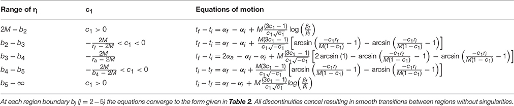
Table 1. Closed-form solution to Equation (12) in Schwarzschild coordinates.

TABLE 2

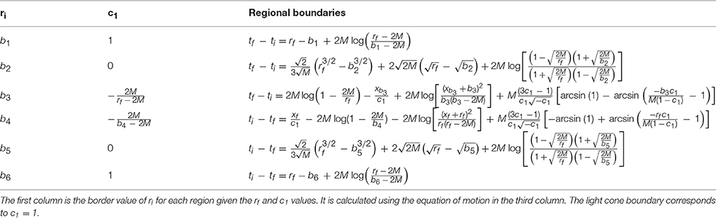
Table 2. Region boundaries for the equation of motion (Equation 12).

The table uses

$\begin{array}{ll}x(r_s)=x_s=\sqrt{c_1{r}_s^2+2M{r}_s(1-c_1)},& (19)\end{array}$

$\begin{array}{ll}{\beta }_s=\sqrt{c_1}{x}_s+c_1{r}_s+M(1-c_1),& (20)\end{array}$

$\begin{array}{ll}{\alpha }_s=\frac{x_s}{c_1}+2M\text{ log}(r_s-2M)-2M\text{ log}\left(\frac{{(r_s+x_s)}^2}{r_s}\right),& (21)\end{array}$

where s = i, f, a.

The direct paths include a logarithmic term when c₁ > 0 and an arc sin term when c₁ < 0. The indirect paths occur for r_i in the b₃ − b₄ region. They each contain a zero velocity point where the path turns around. Mathematically, the velocity passes through zero (dr/dt = 0 at some radius r_a) when x(r_a) = 0, which corresponds to c₁ = −2M/(r_a − 2M). The indirect paths reach the final point (r_f, t_f) after going through a zero velocity point at r_a(t_a < t_f) with r_a > r_f and r_a > r_i. The paths from r_i to r_a correspond to the positive sign in Equation (12), while the path from r_a to r_f corresponds to the negative sign.

To understand these paths we make an analogy with the vertical motion of a ball under gravity (See Figure 1). This analogy arises naturally due to the correspondence between the Friedmann equation and the equation of motion for a test particle in the gravitational field of a point mass in Newtonian gravity. It can be made only in the Schwarzschild case because then the interior of the star can be represented by an FRW model, which provides the link to Newtonian gravity.

FIGURE 1

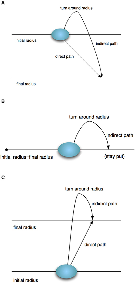
Figure 1. Schematic of paths. (A)r_f < r_i, (B) r_f = r_i, and (C) r_f > r_i.

Consider a ball traveling from point r_i (initial radius) to point r_f (final radius) with r_f below r_i. It can either go down directly from r_i to r_f (direct path) or it can go up from r_i, reach its highest point, where its velocity will be zero, and then fall back down to r_f (indirect path). This is shown schematically in Figure 1A. Analogously, if a ball has to travel from r_i to r_f with r_f above r_i, it can go directly from r_i to r_f or it can pass above r_f, reach its zero velocity point above r_f and return down to r_f. This case can be seen in Figure 1C. The middle figure (Figure 1B) shows the special case when r_i = r_f. Then the ball can either stay put or it can be thrown up, reach its higher point, and fall back down. Each of these paths takes a different amount of time to complete. For a fixed travel time Δt, the two points r_i and r_f are connected by a single path that is either a direct path or a turn-around path. At the turning point of a turn-around path (also its highest point) the speed of the particle is always zero.

If we keep the time interval constant, we find that for a given r_f there is a point r_i = b₄ > r_f, where the velocity dr/dt at b₄ = 0. Similarly, there is a point r_i = b₃ < r_f such that the velocity dr/dt at r_f = 0. For any point r_i between b₃ and b₄, the only way a particle can reach r_f in the same time Δt is if it goes through a turning point r_a > r_f and r_a > r_i. The particle cannot reach r_f > r_i if it's velocity vanishes at any point between r_i and r_f.

The motion toward or away from r = 2M can be compared to the vertical motion of a ball under gravity when thrown straight down or up, respectively. Classically, the star will always collapse to a black hole. Quantum mechanically, we include all possible initial velocities of the surface of the star toward and away from 2M. The wavefunction of a particle on the surface of the star determines the spread of the trajectory of the surface of the star itself.

3.3. Escape Velocity

For a particle of mass m that is thrown up from the surface of the Earth, an initial upward velocity v_escape ≥ 11.2 km/s ensures that the particle escapes Earth gravity. At this speed

$\begin{array}{ll}\frac{G{M}_{E}m}{R_E}=\frac{m{v}_i^2}{2},& (22)\end{array}$

where M_E, and R_E are the Earth mass and radius.

We continue with the ball analogy to estimate the escape velocity for our particle. In our case, R_E is replaced by the initial radius of the star r_i, and v_i = dr/dτ. The kinetic energy of the particle on the surface of the star equals its potential energy when

$\begin{array}{ll}\frac{Mm}{r_i}=\frac{m}{2}{\left|\frac{dr}{d\tau }\right|}_{r=r_i}^2.& (23)\end{array}$

Here

$\begin{array}{ll}\frac{dr}{d\tau }={\left(1-\frac{2M}{r}\right)}^{-1}\frac{dr}{dt}& (24)\end{array}$

with dr/dt = $\dot{r}$ given by Equation (11). This results in

$\begin{array}{ll}\frac{Mm}{r_i}=\frac{m{c}_1}{2}+\frac{Mm}{r_i}(1-c_1),& (25)\end{array}$

whose solution is c₁ = 0. So, while all outgoing paths with c₁ < 0 will turn-around, outgoing paths with c₁ ≥ 0 will not have turning points. When c₁ = 0, the turning point (dr/dτ|_ra = 0, x_a = 0) occurs at r_a → ∞ as expected for an escaped particle.

The different paths (Table 1) and their various regional boundaries (Table 2) are summarized below for a given (r_f, t_f) outside r = 2M:

• c₁ = 1: the paths are light-like (ds² = 0) with r_i = b₁ < r_f and r_i = b₆ > r_f. The paths with c₁ > 1 are space-like, while those with c₁ < 1 are time-like.

• c₁ = 0: r_i = b₂ < r_f and r_i = b₅ > r_f. This path defines the escape velocity. All paths with c₁ > 0 that are outgoing will not reverse, allowing the particle to escape the gravity of the star.

• c₁ = −2M/(r_f − 2M): r_i = b₃ < r_f. The minimum value of r_i where r_f is reached directly with x(r_f) = 0 and null final velocity

$\frac{dr}{dt}{|}_{r=r_f}=0.$

Paths with r_i ≤ b₃ are direct. Paths with r_i between b₃ and b₄ are indirect.

• c₁ = −2M/(b₄ − 2M): r_i = b₄ > r_f. This path starts with zero initial velocity. All paths with r_i > b₄ are direct.

4. Classical Paths in Kruskal Coordinates

Our study is the first to consider space-like paths in Kruskal coordinates for a particle on the surface of a collapsing star. They have not been explicitly considered before because they are believed to be of low probability. We conjecture that they play an important role in quantum mechanical collapse in the same way the probability of passing through the potential barier is important in tunneling. Classically, it can never happen, and yet this probability cannot be ignored in quantum mechanics.

In this section we derive and discuss the closed-form solutions to the equation of motion for the space-like, light-like and time-like paths in Kruskal coordinates. We find that space-like geodesics have the interesting property that they can turn around outside r = 2M and move back in time. Unlike the Schwarzschild t and r, which are time and space coordinates, respectively, outside r = 2M but switch roles for r < 2M, the Kruskal coordinate v is always a time coordinate and the coordinate u is always a space coordinate. The relation between the Schwarzschild r and t and the Kruskal variables u and v is given by

$u=\{\begin{array}{ll}\sqrt{\frac{r}{2M}-1}{e}^{r/4M}\cosh \frac{t}{4M}\hfill & r>2M\hfill \\ \sqrt{1-\frac{r}{2M}}{e}^{r/4M}\sinh \frac{t}{4M}\hfill & r<2M\hfill \end{array}$

$v=\{\begin{array}{ll}\sqrt{\frac{r}{2M}-1}{e}^{r/4M}\sinh \frac{t}{4M}\hfill & r>2M\hfill \\ \sqrt{1-\frac{r}{2M}}{e}^{r/4M}\cosh \frac{t}{4M}\hfill & r<2M\hfill \end{array}$

with

$\begin{array}{ll}{u}^2-v^2=\left(\frac{r}{2M}-1\right)e^{r/2M}& (26)\end{array}$

and

$\begin{array}{ll}\frac{v}{u}=\text{tanh}\frac{t}{4M},r>2M& (27)\\ \frac{u}{v}=\text{tanh}\frac{t}{4M},r<2M.\end{array}$

Thus the line element in Kruskal coordinates takes the form

$\begin{array}{ll}d{s}^2=\frac{32M^3}{r}{e}^{-r/2M}\left(d{u}^2-d{v}^2\right)+r^{2}d{\Omega }^2.& (28)\end{array}$

The singularity at r = 0 occurs at u² − v² = −1. In this paper we consider only the first quadrant u > 0 and v > 0. The horizon r = 2M occurs at u = v. Outside the horizon u > v, whereas inside the horizon u < v.

The classical equation of motion

$\begin{array}{ll}\frac{\ddot{u}}{1-{\dot{u}}^2}=\left(1-\frac{4M^2}{r^2}\right)\frac{u-v\dot{u}}{u^2-v^2}& (29)\end{array}$

can be derived from the Euler-Lagrange equations

$\begin{array}{ll}\frac{d}{dv}\frac{\partial {L}}{\partial \dot{u}}-\frac{\partial {L}}{\partial u}=0,& (30)\end{array}$

for the Lagrangian

$\begin{array}{ll}{L}(u,\dot{u},v)=-4M\sqrt{\frac{(1-{\dot{u}}^2)(1-2M/r)}{(u^2-v^2)}}.& (31)\end{array}$

Note that here $\dot{u}=du/dv$.

The equation of motion can be reduced to

$\begin{array}{ll}\frac{du}{dv}=\frac{v/u\pm x_r/r}{1\pm (v/u)(x_r/r)},& (32)\end{array}$

where x_r is given by Equation (13). Direct paths from r_i to r_f > r_i have the “+”-sign in the numerator and denominator with du/dv > 0. Direct paths from r_i to r_f with r_f < r_i will have the “−”-sign in the numerator and denominator.

The classical paths describing the evolution of the star outside r = 2M have been discussed in Sec. 3.2 in Schwarzschild coordinates. It was shown that there were direct space-like and light-like paths as well as direct and indirect time-like paths. Any two points in (r, t) were connected by a unique classical path.

What is new in Kruskal space-time are the turning points in the u − v plane for all space-like, light-like and time-like paths. Spacelike paths (c₁ > 1, |du/dv| > 1) turn in time at points when dv/du = 0, whereas timelike paths (c₁ < 1, |du/dv| < 1) turn in space when du/dv = 0. Additionally, there are indirect space-like and light-like paths that have turning points in r inside the apparent horizon (here we refer to paths as being indirect when they turn in r; the light-like paths turn at r = 0). In contrast to the time-like paths, the in-going space-like paths are not unique. A point outside r = 2M might be connected to a point inside the apparent horizon via a direct and an indirect space-like path or via two indirect space-like paths.

We determine the regions (Table 3) and the light-cone boundaries (Table 4) that delimit the different kinds of paths that start at (u_i, v_i = 0) outside the horizon and reach (u_f, v_f) inside the apparent horizon. Outside the horizon, the light cone boundary values of “u_i” for a given u_f and v_f can be determined by replacing t_f − t_i in Table 2 by ${\text{tanh}}^{-1}(v_f/u_f)$. The boundary values of r_i (v_i = 0) with r_f < 2M, are calculated from the equations in Table 4. Note that u_f is a function of v_f and r_f and u_i depends on v_i, which is typically taken to be zero, and r_i. Thus if one finds r_i, this determines u_i. The point $r_i=b_4^{\prime }$ corresponds to x_i = 0 with $c_1=-2M/(b_4^{\prime }-2M)$. The c₁ = 0 and c₁ = 1 (lightlike) paths that reach points (u_f, v_f) inside the horizon are used to determine the r_i values $b_5^{\prime }$ and $b_{56}^{\prime }$, respectively. The $r_i=b_6^{\prime }$ value corresponds to x_f = 0 with c₁ = −2M/(r_f − 2M) (turning point at r = r_f < 2M, space-like path, c₁ > 1). The value of $r_i=b_7^{\prime }$ is to be determined by using c₁ = −2M/(r_a − 2M) (x_a = 0, r_a < r_f < 2M) in the equation of motion. The two unknowns $b_7^{\prime }$ and r_a are determined by using the equation of motion and its partial derivative with respect to c₁. Both equations are given in Table 4. In the region outside $b_7^{\prime }$ ($r_i>b_7^{\prime }$), there exist no classical paths to (u_f, v_f).

TABLE 3

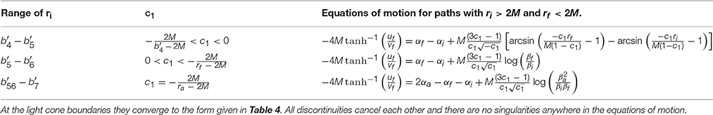
Table 3. The equation of motion with r_f < 2M.

TABLE 4

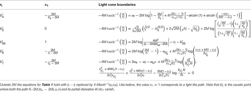
Table 4. Equations of motion at light cone boundaries for paths with r_f < 2M.

In Figures 2A,B we trace direct time-like, direct space-like, and indirect space-like trajectories that start at v_i = 0 and pass through a fixed point P(u_P = 9.995, v_P = 10.0) with r_P ≈ 0.8M, which is located inside the apparent horizon. Path 1 and path 2 are time-like, and originate at different points outside r = 2M. Path 1 (u_i = 2.59, c₁ = −1.05) lies in the $b_4^{\prime }-b_5^{\prime }$ region of Table 3. Path 2 (u_i = 16.15, c₁ = 0.8) lies in the $b_5^{\prime }-b_{56}^{\prime }$ region, which contains time-like paths with a turning point in the u − v plane (du/dv = 0) that lies outside the apparent horizon.

FIGURE 2

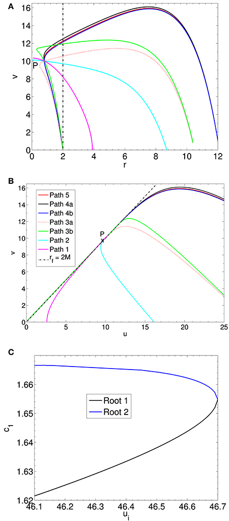
Figure 2. (A) v vs. r and (B) v vs. u are shown for space-like and time-like paths with v_i = 0 that pass through P(u_P = 9.995, v_P = 10.0) of r_P = 0.8, a point located inside the apparent horizon. (C) The c₁ values for indirect space-like paths in the region between $b_6^{\prime }$ and $b_7^{\prime }$ from which point P can be reached are displayed for each u_i. No paths exist beyond $r=b_7^{\prime }$, which is where the two roots merge into one.

The next region is $b_{56}^{\prime }-b_6^{\prime }$, where each point outside the horizon is connected to points inside the horizon by two space-like paths: one direct and one indirect. Path 3a and path 3b originate at the same u_i = 27.6 (r_i = 10.5M). Path 3a reaches P directly. However, after having passed through P, it turns at r_a = 0.48M before reaching the horizon like all space-like paths. Path 3b is indirect turning at r_a = 0.3M (u_a = 11.3, v_a = 11.35), and then reaching P on its way back toward the apparent horizon. Both paths also have a v − u turning point outside the apparent horizon where dv/du = 0. After having passed through its v − u turning point, each path moves back in time (the space coordinate u continuously decreases, while the time coordinate v increases up to the turning point and then decreases).

In the $r_i=b_6^{\prime }-b_7^{\prime }$ region there are two indirect paths that connect the same point outside the horizon to a point inside r = 2M. Paths 4a and 4b connect the point of u_i = 46.3 to P. They each have a dv/du = 0 turning point outside the horizon, and also turn in r inside the horizon before reaching P. Path 4a turns at r_a = 0.77147 < r_P and path 4b turns at r_a = 0.79969 < r_P. It can be seen that the paths are very close together. As u_i increases, the paths in this region become progressively closer until they merge at $r_i=b_7^{\prime }$. Path 5 shows the single indirect path that originates at u_i = 46.7 ($r_i=b_7^{\prime }=12.13M$). Beyond this point, there are no real solutions and hence no way to reach point P.

Figure 2C displays the c₁ values of space-like paths reaching point P (u_P = 9.995, v_P = 10.0) from u_i ≥ 46.1 at v_i = 0. At first, for each u_i in the figure there are two c₁ values with which the final point P can be reached. The figure clearly shows the roots (c₁ values) coming closer and closer together until they merge at the caustic point $r=b_7^{\prime }$. Beyond this point there are no paths that reach point P. Extensions to this work to determine the Kruskal-WKB wavefunction will require an analysis of the caustic at $r=b_7^{\prime }$ to remove any potential divergences.

The indirect paths connecting (u_i, v_i) with r_i > 2M to (u_P, v_P) with r_P < 2M penetrate the horizon deeper than r_P turning at r_a < r_P before reaching r_P (e.g., see the green path in Figure 2A). After turning, all paths must continue toward the apparent horizon reaching it at u = v = 0. These paths move back in time from a point outside the horizon, where dv/du = 0, after having traveled to that point forward in Kruskal time from (u_i, v_i = 0) with r_i > 2M.

As discussed before, the turning points in r correspond to x_r = 0 (in the Kruskal paths x_r appears in Equation 58). They occur at r = r_a when x_a = 0, where c₁ = − 2M/(r_a − 2M). Since c₁ > 1 for space-like paths, clearly r_a < 2M (the turning points are inside the horizon). For any r on a path with r_a as the turning point, x_r can be written as $\sqrt{2Mr(r-r_a)/(2M-r_a)}$. To ensure the non-negativity of the term under the square root all points on this path must have r > r_a. By the same token, for time-like paths r_a > 2M and r < r_a. This case was described in the Schwarzschild analysis.

All space-like paths that reach points inside the horizon subsequently head toward the horizon r = 2M (u = v). Classically, they end at u_f = v_f = 0. However, quantum mechanically there may be paths close to the classical path that bring information from within the black hole horizon to the outside.

5. Quantum Treatment in Schwarzschild Coordinates

We consider a collapsing cloud of ultra-light particles with mM ~ ℏ. Such particles are not localized and thus neither is the surface of the star. The position of a particle on the surface of the star is then approximated by a wavefunction. In a relativistic path integral approach, this wavefunction can be computed in the WKB approximation via an integral over the classical action (Schulman, 2005). It is necessary to include configurations will all possible initial velocities. For each point (r_f, t_f) all classical paths derived above are needed. In this paper, we only perform the WKB analysis in Schwarzschild coordinates, where we can only use the paths to r_f > 2M.

5.1. WKB Approximation: Closed-Form Propagator, Numerical Wavefunction

In order to study the wavefunction we use a WKB approximation of the propagator

$\begin{array}{ll}G(r,t;r_i,t_i)={\displaystyle {{\displaystyle \int }}_C}{D}r\text{ exp}\left[iS/\hslash \right],& (33)\end{array}$

where S is the action associated with each path. The set of paths C include space-like, time-like and light-like paths.

The WKB approximation involves expanding about the classical action S_cl to include paths that slightly deviate from the classical paths. The propagator is dominated by paths near the classical trajectory between (r_i, t_i) and (r, t) and is approximated by the WKB expression (Schulman, 2005)

$\begin{array}{ll}{G}_{\text{WKB}}(r,t;r_i,t_i)=\sqrt{\frac{i}{2\pi \hslash }\frac{{\partial }^2{S}_{\text{cl}}}{\partial r_i\partial r_f}}\text{exp}\left(i\frac{S_{\text{cl}}}{\hslash }\right).& (34)\end{array}$

The WKB wave function is obtained from the integration of the propagator

$\begin{array}{ll}{\text{Ψ}}_{\text{WKB}}(r_f,t_f)={\displaystyle {{\displaystyle \int }}_0^{\infty }}{G}_{\text{WKB}}(r_f,t_f;r_i,t_i)\text{Ψ}(r_i,t_i)d{r}_i.& (35)\end{array}$

The initial wavefunction that describes a particle on the surface of a star of radius r_i is taken to be a Gaussian centered about r_c

$\begin{array}{ll}\text{Ψ}(r_i,t_i=0)=\text{exp}\left[-\frac{{\left(r_i-r_c\right)}^2{m}^2}{{\hslash }^2}\right]& (36)\end{array}$

with r_c >> 2M.

The action from Equation (6) is rewritten using Equations (11) and (13) as

$\begin{array}{ll}{S}_{\text{cl}}(r_i,t_i;r_f,t_f)=\pm im\sqrt{c_1-1}{\displaystyle {{\displaystyle \int }}_{(r_i,t_i)}^{(r_f,t_f)}}dr\frac{r}{x(r)}& (37)\end{array}$

for direct paths connecting (r_i, t_i) to (r_f, t_f). The + sign corresponds to r_f > r_i and the − sign corresponds to r_f < r_i.

Indirect paths connecting (r_i, t_i) to (r_f, t_f) through the turning point (r_a, t_a) with r_a > r_i and r_a > r_f are described by the classical action

$\begin{array}{ll}{S}_{\text{cl}}=im\sqrt{c_1-1}\left[{\displaystyle {{\displaystyle \int }}_{(r_i,t_i)}^{(r_a,t_a)}}dr\frac{r}{x(r)}-{\displaystyle {{\displaystyle \int }}_{(r_a,t_a)}^{(r_f,t_f)}}dr\frac{r}{x(r)}\right].& (38)\end{array}$

In Schwarzschild coordinates, the wavefunction is continuous across all regions outside r = 2M. The presence of the r = 2M coordinate singularity prohibits the inclusion of paths at or beyond the horizon region. Closed-form expressions for S_cl and ${\partial }^2{S}_{\text{cl}}/(\partial r_i\partial r_f)$ are given in Table 5. Both functions are continuous across all regions outside r = 2M. Once c₁ is known for every point (r, t), we have all the ingredients to find the propagator in Equation (34) using the S_cl, and ${\partial }^2{S}_{\text{cl}}/\partial r_i\partial r_f$ expressions from Table 5. The propagator is then integrated to find the wavefunction.

TABLE 5

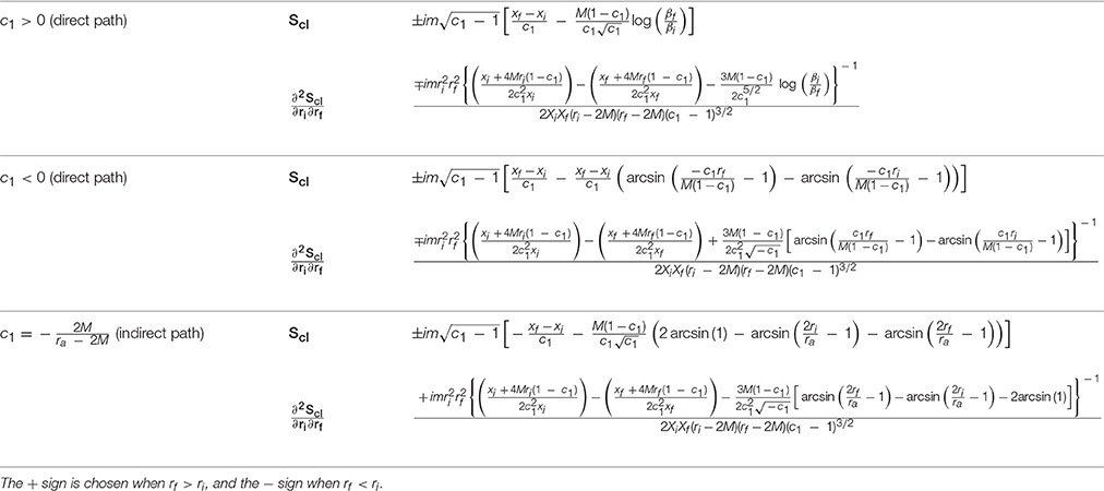
Table 5. The classical action in various regions.

5.2. Relativistic Schrödinger Solution

5.2.1. Free Particle

The M → 0 limit describes a relativistic free particle that is no longer confined by the gravity of the sphere of dust. This case was first studied by Redmount and Suen (1993). We revisit this limit to investigate whether the wavefunction in the WKB approximation converges to the relativistic Schrödinger solution, which is the exact solution for this case. In Redmount and Suen (1993) some disagreement was observed, but while they attempted a physical interpretation, it is likely due to numerical error.

When M → 0, the Hamiltonian from Equation (9) reduces to

$\begin{array}{ll}H=\sqrt{{\text{p}}^2+m^2},& (39)\end{array}$

where p is now the momentum operator. The Hamiltonian is nonpolynomial in p. The square root term thus corresponds to a non-local momentum operator that is interpreted as acting on any wavefunction (Redmount and Suen, 1993)

$\begin{array}{ll}\text{Ψ}(x,t)={\displaystyle {{\displaystyle \int }}_{-\infty }^{\infty }}dk{e}^{ikx}\varphi (k,t).& (40)\end{array}$

to give

$\begin{array}{ll}H\text{Ψ}(x,t)={\displaystyle {{\displaystyle \int }}_{-\infty }^{\infty }}dk{e}^{ikx}\sqrt{{\hslash }^2{k}^2+m^2}\varphi (k,t).& (41)\end{array}$

This integrates to

$\begin{array}{ll}\varphi (k,t)=A(k,x_0)\text{exp}\left(-\frac{i\Delta t}{\hslash }\sqrt{{\hslash }^2{k}^2+m^2}\right).& (42)\end{array}$

When Δt = 0, we recover the original wavefunction, which is chosen to be a Gaussian centered around the origin,

$\begin{array}{l}\text{Ψ}(x_0,t_0)={N}\text{ exp}\left(-\frac{m^2{x}_0^2}{{\hslash }^2}\right),\end{array}$

and so

$\begin{array}{ll}\text{Ψ}(x,t)=\frac{{N}}{2\pi }{\displaystyle {{\displaystyle \int }}_{-\infty }^{\infty }}dk{\displaystyle {{\displaystyle \int }}_{-\infty }^{\infty }}d{x}_0\text{ exp}\left(-m^2{x}_0^2/{\hslash }^2\right)& (43)\\ \times \text{exp}\left(ik\Delta x\right)\text{exp}\left(-\frac{i\Delta t}{\hslash }\sqrt{{\hslash }^2{k}^2+m^2}\right).\end{array}$

The normalization $|{N}{|}^2=m\sqrt{2}/(\hslash \sqrt{\pi })$ is time independent.

In terms of the propagator

$\begin{array}{ll}\text{Ψ}(x_f,t_f)={\displaystyle {{\displaystyle \int }}_{-\infty }^{\infty }}d{x}_{0}G(x_f,t_f;x_0,t_0)\text{Ψ}(x_0,t_0),& (44)\end{array}$

where

$\begin{array}{l}G(x,t;x_0,t_0)={\displaystyle {{\displaystyle \int }}_{-\infty }^{\infty }}\frac{dk}{2\pi }\text{exp}\left(ik\Delta x\right)\hfill \\ \times \text{exp}\left[-\frac{i\Delta t}{\hslash }\sqrt{{\hslash }^2{k}^2+m^2}\right],\hfill \\ ={\displaystyle \underset{ϵ\to 0^{+}}{\text{lim}}}\frac{m(i\Delta t+ϵ)}{\pi \hslash \sqrt{{\lambda }_{ϵ}}}{K}_1(m{\lambda }_{ϵ}^{1/2}/\hslash ).\hfill & (45)\end{array}$

Here K₁ is the modified Bessel function and ${\lambda }_{ϵ}\equiv \Delta x^2+{(i\Delta t+ϵ)}^2$. When Δt = 0 the propagator reduces to δ(Δx) as expected.

The WKB propagator for the relativistic free particle is then computed using Equation (34) Redmount and Suen (1993)

$\begin{array}{ll}{G}_{WKB}=\sqrt{\frac{m}{2\pi }\frac{{(i\Delta t+ϵ)}^2}{\hslash {\lambda }_{ϵ}^{3/2}}}\text{exp}\left[-\frac{m{\lambda }_{ϵ}^{1/2}}{\hslash }\right],& (46)\end{array}$

where WKB wavefunction is given by

$\begin{array}{ll}{\text{Ψ}}_{WKB}(x,t)={\displaystyle {{\displaystyle \int }}_{-\infty }^{\infty }}d{x}_0{G}_{WKB}(x,t;x_0,t_0)\text{Ψ}(x_0,t_0).& (47)\end{array}$

The integrals from Equations (44) and (47) are evaluated numerically. The results are shown in Figure 3. It can be seen that the wavefunction in the WKB approximation converges to the Schrödinger solution in all parts of the light cone. When no star M is present, the relativistic Schrödinger is exact as originally discussed in Redmount and Suen (1993). However, when they performed the same numerical comparison, they found some disagreement between the two solutions. This we believe to be due to numerical error of Redmount and Suen (1993). We observe convergence (see Figure 3). of the wavefunction in the WKB approximation to the Schrödinger solution in the M → 0 limit.

FIGURE 3

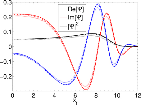
Figure 3. Re[Ψ], Im[Ψ], and |Ψ|² are shown for the free particle case at t = 10ℏ/m as a function of x_f, which also has units of ℏ/m. The solid lines show the Schrödinger solution, while dotted lines and dashed lines show the WKB approximation for ϵ = 0.05, ϵ = 0.005, respectively. It can be seen that as ϵ → 0 the WKB approximation converges to the Schrödinger solution.

5.2.2. Non-zero Mass

While in the free particle case the Schrödinger solution was exact, when M ≠ 0 it becomes a rough approximation, which fails as we approach r = 2M. Comparing the two solutions is still instructive. If we follow the same procedure as for the free particle above, and re-write the Hamiltonian from Equation (9) as

$\begin{array}{ll}H=\sqrt{B^2{\text{p}}^2+B{m}^2},& (48)\end{array}$

where p is the momentum operator and

$\begin{array}{ll}B=B(M,r)=1-\frac{2M}{r}.& (49)\end{array}$

The whole wavefunction can then be written as

$\begin{array}{ll}\text{Ψ}(r,t)={\displaystyle \int }d{r}_{i}G(r,t;r_i,t_i)\text{Ψ}(r_i,{\tau }_i),& (50)\end{array}$

where the propagator is given by

$\begin{array}{ll}G(r,t;r_i,t_i)={\displaystyle {{\displaystyle \int }}_{-\infty }^{\infty }}\frac{dk}{2\pi }\text{exp}(ik\Delta r)& (51)\\ \times \text{exp}\left[-i\frac{\Delta t}{\hslash }\sqrt{{\hslash }^2{k}^2{B}^2+m^{2}B}\right].\end{array}$

Like before, the propagator can then be integrated exactly to obtain

$\begin{array}{ll}G(x,t;x_i,t_i)={\displaystyle \underset{ϵ\to 0}{\text{lim}}}\frac{m(i\Delta t+ϵ)}{\pi \hslash B^{1/2}{\lambda }_{ϵ}^{1/2}}{K}_1(m{B}^{1/2}{\lambda }_{ϵ}^{1/2}/\hslash ),& (52)\end{array}$

where K₁ is the modified Bessel function and

$\begin{array}{ll}{\lambda }_{ϵ}={\left(\frac{\Delta r}{B}\right)}^2+{(i\Delta t+ϵ)}^2.& (53)\end{array}$

When r → 2M the propagator vanishes. Thus this solution is inaccurate at late times and cannot model the final stages of the collapse of the dust sphere.

5.3. Numerical Results

We integrate Equation (35) numerically for the Gaussian wavefunction from Equation (36) centered about r_c = 30M. Classically, the star collapses to r = 2M in infinite Schwarzschild time. However, quantum mechanically there is a possibility for the star expanding and dispersing as well. Figure 4 shows the time evolution from t = 0 to t = 45M of $|{\text{Ψ}}_{WKB}(r_f,t_f){|}^2$ as a function of r_f. An ingoing peak and an outgoing peak appear with the amplitude of the ingoing peak always remaining larger than that of the outgoing peak for the course of the evolution, which is expected for a collapsing star. For numerical computations we scale all variables to be dimensionless. The only parameter is mM/ℏ. We note that Figure 4 is qualitatively similar to the WKB results of Corichi et al. (2002).

FIGURE 4

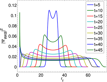
Figure 4. The time evolution of WKB $|\text{Ψ}(r_f,t_f){|}^2$ is shown from t = 5M to t = 45M in the case of mM/ℏ = 1. We can see that the star collapses to a black hole.

Figures 5A,B show the ingoing and outgoing peaks of $|{\text{Ψ}}_{WKB}(r,t_f){|}^2$ for different values of mM/ℏ at times of t_f = 5M and t_f = 10M, respectively. For a given particle number N = M/m, the speed of the collapse increases slightly with the particle mass m as does the value of the ingoing peak. This is consistent with our expectation that for higher particle mass the star is more classical. For lower masses, the star resists collapse longer until probability of dispersion exceeds the probability of collapse.

FIGURE 5

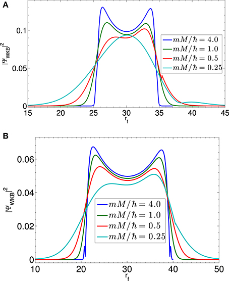
Figure 5. (A) $|\text{Ψ}(r_f,t_f){|}^2$ at t = 5M as a function of r_f for mM/ℏ = 4.0, mM/ℏ = 1, mM/ℏ = 0.5, and mM/ℏ = 0.25. It can be seen that that lower masses behave more quantum mechanically, and are less likely to collapse to a black hole. (B) $|\text{Ψ}(r_f,t_f){|}^2$ at t = 10M as a function of r_f for the same masses.

In Figure 6 we compare the WKB and Schrödinger solutions. It can be seen that the radial position of the ingoing peak drifts out of step at late times, while the outgoing peak continues to evolve at about the same position. As the star approaches r_f = 2M, the ingoing peak amplitude for the WKB approximation increases developing a numerical singularity that indicates the formation of an apparent horizon, while the ingoing peak amplitude of the Schrödinger solution decreases since the propagator in Equation (52) vanishes at r_f → 2M. The latter behavior reinforces that the relativistic Schrödinger equation is not the correct representation for a particle in the gravitational field of a collapsing star.

FIGURE 6

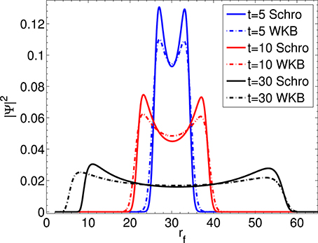
Figure 6. mM/ℏ = 1 Schrödinger (solid line) and WKB comparison (dotted line).

6. Conclusion

Closed form solutions for the classical paths taken by a particle on the surface of a collapsing star have been determined for all initial configurations in Schwarzschild and Kruskal coordinates.

We found that

(i) all time-like paths are unique. For a given time interval, a path between an initial and final point can be either direct or indirect, where it turns around in space. Thus some particles that initially move away from the star, can return and contribute to the collapse.

(ii) all space-like paths are unique outside r = 2M.

(iii) Kruskal space-like paths can turn around in Kruskal time, but cannot turn in Kruskal space. Multiple paths can connect a given point outside the horizon to a final point that lies inside r = 2M.

(iv) Classical Kruskal space-like paths connect points outside r = 2M with points inside r = 2M up to a critical value of r = r_a. Spacelike paths from (r_i, v_i = 0) to any given point r inside the horizon, where r_a < r < 2M, are non-unique (two paths exist). These paths get less and less separated and merge into a single space-like path at r = r_a and any point r < r_a is unreachable from r_i. Upon reaching the critical value r = r_a, the space-like paths turn back toward r = 2M, reaching it at u = v = 0. Therefore, classically, no information from r < 2M can exit a black hole. However, by taking into account paths close to the classical paths, one might be able to extract information from r < 2M.

If we make an analogy to tunneling, the particle has a low probability of passing through a potential barier. Classically, it never happens, and yet this probability cannot be ignored in quantum mechanics. Similarly, it may be that the low probability space-like paths will play a crucial role in our understanding of quatum mechanical collapse.

The collapse of a self-gravitating star was next modeled as a ball of dust using a WKB approximation. We integrated around the classical paths with all possible initial velocities to include quantum effects. This extended the analysis of Redmount and Suen (1993) from the relativistic free particle to the case of non-trivial gravity. In practice, quantum mechanical effects are important in macroscopic stellar collapse when the sphere is composed of ultra-light particles. A number of ultralight dark matter particles have been proposed, which could physically motivate such stars.

The evolution of the wavefunction of a particle on the surface of a collapsing star was followed numerically. We showed that in the case of a star collapsing with zero initial velocity, our path equations reduce to the Oppenheimer-Schneider equations of motion. In the M → 0 limit, the relativistic free particle wavefunction of Redmount and Suen (1993) is obtained, and the WKB and relativistic Schrödinger solutions match. Since in this limit the Schrödinger solution is exact (Kiefer and Singh, 1991), the covergence of the WKB to the Schrödinger solution enforces the validity of the WKB approximation.

Our results for this self-gravitating collapse are summarized as follows:

(i) The wavefunction representing a particle on the surface of a collapsing star typically exhibits an outgoing and an ingoing component, where the former contains the probability that the star will disperse and the latter the collapse probability. For a given particle number N = M/m, we find that the rate at which collapse occurs increases with particle mass. This is consistent with the expectation that for higher particle mass the star is more classical. As the particle mass is lowered, the star resists collapse until the probability that it disperses exceeds the collapse probability. Note that some part of the star always disperses even when a black hole forms.

(ii) In the case of the collapsing star the relativistic Schrödinger solution is not a good approximation for the wave function. On comparing the WKB and relativistic Schrödinger solutions, we find that the ingoing wavefunction gets more and more out of step at late times. The outgoing component of the wavefunction for the two solutions is in better agreement because it is further from the coordinate singularity at r = 2M. As expected, the Schrödinger and WKB solutions are out of step at early times when WKB solution is more inaccurate, they come closer together at intermediate times, and fall out of step again at late times, when the Schrödinger approximation fails to model the singularity formation. The presence of the coordinate singularity at r = 2M, motivate a potential investigation beyond r = 2M via the WKB approximation deployed in Kruskal coordinates where no analytical relativistic Schrödinger solution is available.

The traditional Oppenheimer Schneider model describes the zero pressure collapse of a star starting from rest. We use a path integral approach that requires including paths of all velocities. For a particle on the surface of a star, we explicitly parametrically describe all such paths of different initial velocities. This is done in Schwarzschild coordinates until r = 2M and in Kruskal coordinates until the r = 0 singularity. We include ingoing and outgoing velocities, and time-like, light-like and space-like paths. In the process we have generated the paths shown in Fuller and Wheeler (1962) and more. We have determined equations for the space-like caustics (degenerate paths) which have not been described before in this manner. We have used a WKB path integral approach and determined the Schwarzschild wave function for the collapse. Using a similar approach one can in the future use the parametric path equations we have determined in Kruskal coordinates to explore the space-time inside the horizon. It will require expansion around the caustic. The possibility of paths moving back in time might have important ramifications.

It has long been argued whether quantum gravity should be causal or not (Teitelboim, 1983; Hartle and Kucha, 1986; Hartle, 1988; Mattingly, 2005) and as of today there is no accepted theory of quantum gravity. We evaluate the propagator both for a free relativistic particle, where we have an exact solution, and for a collapsing ball of dust. Since the propagator does not vanish outside the light cone, we include all paths in our integration. In the free particle case, the WKB and exact solutions match. Space-like classical paths give the dominant contribution in the construction of the WKB approximation far outside the light cone, where the approximation is valid. This propagation will be acausal (backward in time) in some Lorentz frames. Whether or not this proves to be admissible in the ultimate theory of quantum gravity is beyond the purpose of our work. Our work's exploration of the consequence of an acausal propogator in the collapse of a zero pressure star might nevertheless contribute to the dialogue in the search of a consistent theory of quantum gravity.

In addition, we propose that an understanding of these low probability paths that are traditionally ignored could shed some light in theories of black hole formation. Furthermore, if the black holes observed by LIGO are formed from scalar particles (Abbott et al., 2016), the particles would be very light; then quantum effects might play a role in their formation, constraining analog gravity theorems (Barceló et al., 2005).

Author Contributions

All authors listed, have made substantial, direct and intellectual contribution to the work, and approved it for publication.

Conflict of Interest Statement

The authors declare that the research was conducted in the absence of any commercial or financial relationships that could be construed as a potential conflict of interest.

Acknowledgments

JB acknowledges Prof. Wai-Mo Suen for the initial impetus to approach this research and for subsequent guidance and useful discussions. We also thank Prof. Ian Redmount for his inital work on this topic. Further, we are particularly grateful to Prof. Mihai Bondarescu and Prof. Philippe Jetzer for useful discussions and advice. RB has received support from the Dr. Tomalla Foundation and the Swiss National Science Foundation. CM is supported by the NSF Astronomy and Astrophysics Postdoctoral Fellowship under award AST-1501208.

References

Abbott, B., Abbott, R., Abbott, T. D., Abernathy, M. R., Acernese, F., et al. (2016). Astrophysical implications of the binary black hole merger gw150914. Astrophys. J. Lett. 818:L22. doi: 10.3847/2041-8205/818/2/L22

CrossRef Full Text | Google Scholar

Alberghi, G., Casadio, R., Vacca, G., and Venturi, G. (1999). Gravitational collapse of a shell of quantized matter. Class. Quantum Grav. 16, 131.

Google Scholar

Ansoldi, S., Aurilia, A., Balbinot, R., and Spallucci, E. (1997). Classical and quantum shell dynamics, and vacuum decay. Class. Quantum Grav. 14, 2727. doi: 10.1088/0264-9381/14/10/004

CrossRef Full Text | Google Scholar

Barceló, C., Liberati, S., and Visser, M. (2005). Analogue gravity. Living Rev. Relativ. 8, 214. doi: 10.12942/lrr-2005-12

CrossRef Full Text

Berezin, V. A. (1997). Quantum black hole model and Hawking's radiation. Phys. Rev. D 55, 2139.

Google Scholar

Casadio, R., and Venturi, G. (1996). Semiclassical collapse of a sphere of dust. Class. Quantum Grav. 13, 2715.

Google Scholar

Corichi, A., Cruz-Pacheco, G., Minzoni, A., Padilla, P., Rosenbaum, M., Ryan, M. Jr., et al. (2002). Quantum collapse of a small dust shell. Phys. Rev. D 65:064006. doi: 10.1103/PhysRevD.65.064006

CrossRef Full Text | Google Scholar

Dolgov, A., and Khriplovich, I. (1997). Properties of the quantized gravitating dust shell. Phys. Lett. B 400, 12–14. doi: 10.1016/S0370-2693(97)00352-3

CrossRef Full Text | Google Scholar

Fuller, R. W. Wheeler, J. A. (1962). Causality and multiply connected space-time. Phys. Rev. 128:919. doi: 10.1103/PhysRev.128.919

CrossRef Full Text | Google Scholar

Goswami, R., and Joshi, P. S. (2004). Spherical dust collapse in higher dimensions. Phys. Rev. D 69:044002. doi: 10.1103/PhysRevD.69.044002

CrossRef Full Text | Google Scholar

Hájíček, P., Kay, B. S., and Kuchar, K. V. (1992). Quantum collapse of a self-gravitating shell: equivalence to coulomb scattering. Phys. Rev. D 46:5439. doi: 10.1103/PhysRevD.46.5439

PubMed Abstract | CrossRef Full Text | Google Scholar

Hartle, J. B. (1988). Quantum kinematics of spacetime. II. a model quantum cosmology with real clocks. Phys. Rev. D 38:2985.

PubMed Abstract | Google Scholar

Hartle, J. B., and Kucha, K. V. (1986). Path integrals in parametrized theories: the free relativistic particle. Phys. Rev. D 34:2323.

PubMed Abstract | Google Scholar

Hawkins, E. (1994). Quantum gravitational collapse of a charged dust shell. Phys. Rev. D 49:6556.

PubMed Abstract | Google Scholar

Hu, W., Barkana, R., and Gruzinov, A. (2000). Fuzzy cold dark matter: the wave properties of ultralight particles. Phys. Rev. Lett. 85, 1158–1161. doi: 10.1103/PhysRevLett.85.1158

PubMed Abstract | CrossRef Full Text | Google Scholar

Joshi, P. S. (2007). Gravitational Collapse and Spacetime Singularities. Cambridge, UK: Cambridge University Press.

Google Scholar

Khmelnitsky, A., and Rubakov, V. (2014). Pulsar timing signal from ultralight scalar dark matter. J. Cosmol. Astropart. Phys. 2014:019. doi: 10.1088/1475-7516/2014/02/019

CrossRef Full Text | Google Scholar

Kiefer, C., and Singh, T. P. (1991). Quantum gravitational corrections to the functional schrödinger equation. Phys. Rev. D 44:1067.

PubMed Abstract | Google Scholar

Lesgourgues, J., Arbey, A., and Salati, P. (2002). A light scalar field at the origin of galaxy rotation curves. New Astron. Rev. 46, 791–799. doi: 10.1016/S1387-6473(02)00247-6

CrossRef Full Text | Google Scholar

Lundgren, A. P., Bondarescu, M., Bondarescu, R., and Balakrishna, J. (2010). Lukewarm dark matter: bose condensation of ultralight particles. Astrophys. J. Lett. 715:L35. doi: 10.1088/2041-8205/715/1/L35

CrossRef Full Text | Google Scholar

Mattingly, D. (2005). Modern tests of lorentz invariance. Liv. Rev. Relativ. 8:5. doi: 10.12942/lrr-2005-5

CrossRef Full Text

Misner, C. W., Thorne, K. S., Wheeler, J. A., and Gravitation, W. (1973). Freeman and Company. San Francisco, CA: W.H. Freeman.

Narlikar, J. (1977). Quantum uncertainty in the final state of gravitational collapse. Nature 269:129.

Google Scholar

Oppenheimer, J. R., and Snyder, H. (1939). On continued gravitational contraction. Phys. Rev. 56:455.

Google Scholar

Ortíz, L., and Ryan, M. Jr. (2007). Quantum collapse of dust shells in 2 + 1 gravity. Gen. Relativ. Gravit. 39, 1087–1107. doi: 10.1007/s10714-007-0458-7

CrossRef Full Text | Google Scholar

Redmount, I. H., and Suen, W.-M. (1993). Path integration in relativistic quantum mechanics. Int. J. Mod. Phys. A 8, 1629–1635. doi: 10.1142/S0217751X93000667

CrossRef Full Text | Google Scholar

Schulman, L. S. (2005). Techniques and Applications of Path Integration. Mineola, NY: Courier Dover Publications.

Google Scholar

Singh, T., and Witten, L. (1997). Spherical gravitational collapse with tangential pressure. Class. Quantum Grav. 14:3489.

Google Scholar

Teitelboim, C. (1983). Causality versus gauge invariance in quantum gravity and supergravity. Phys. Rev. Lett. 50:705.

Google Scholar

Vaidya, P. (1951). Nonstatic solutions of einstein's field equations for spheres of fluids radiating energy. Phys. Rev. 83:10.

Google Scholar

Vaz, C., and Witten, L. (2001). Quantum black holes from quantum collapse. Phys. Rev. D 64:084005. doi: 10.1103/PhysRevD.64.084005

CrossRef Full Text | Google Scholar

Zloshchastiev, K. G. (1998). Monopole and electrically charged dust thin shells in general relativity: classical and quantum comparison of hollow and atomlike configurations. Phys. Rev. D 57, 4812–4820.

Google Scholar