Dynamics of orientation tuning in cat V1 neurons depend on location within layers and orientation maps

Introduction

The temporal evolution, or dynamics, of the orientation tuning of responses of V1 neurons can provide insight into the circuit and the mechanisms underlying tuning. Several previous studies have analyzed the orientation tuning dynamics of V1 neurons (Celebrini et al., 1993 ; Chen et al., 2005 ; Gillespie et al., 2001 ; Mazer et al., 2002 ; Nishimoto et al., 2005 ; Ringach et al., 2003 ; Sharon and Grinvald, 2002 ; Shevelev et al., 1993 ; Volgushev et al., 1995 ). In particular, this type of analysis has been used to distinguish between thalamocortical inputs and intracortical excitatory or inhibitory inputs, and thus, to estimate their respective roles in the generation of orientation selectivity. The rationale of such an approach is that the numerous different sources of synaptic input that contribute to the response may be separable in time, and the influence of each may therefore be relatively more prominent at different periods of the response. For instance, if orientation selectivity is generated by the convergence of inputs from the lateral geniculate nucleus (LGN) (Hubel and Wiesel, 1962 ), neurons should be equally selective during the initial and late periods of the response. Alternatively, if orientation selectivity arises from specific intracortical amplification of responses to some orientations, as several models have proposed (Ben-Yishai et al., 1995 ; Douglas et al., 1995 ; Somers et al., 1995 ), the neuron should be less selective during the initial period of the response than later on. Therefore, measurements of the timecourse of response enhancement and suppression may be able to distinguish between these models.

Some studies have demonstrated that the tuning curves derived from early portions of the visual response are quite different from those derived from later in the response (Chen et al., 2005 ; Ringach et al., 2003 ; Sharon and Grinvald, 2002 ; Shevelev et al., 1993 ; Volgushev et al., 1995 ), whereas others have found that orientation selectivity is relatively constant throughout the duration of the visual response (Celebrini et al., 1993 ; Gillespie et al., 2001 ; Mazer et al., 2002 ; Nishimoto et al., 2005 ). We reasoned that different dynamics might result from differences in local cortical inputs. The diversity of results regarding the timecourse of orientation tuning, as well as recent results demonstrating diversity in the mechanisms generating this selectivity (Martinez et al., 2002 ; Monier et al., 2003 ; Schummers et al., 2002 ), suggest that many factors, including cell class, laminar location, and position within the map of orientation preference, may influence the orientation dynamics of V1 neurons.

Here, we describe experiments aimed at clarifying these issues by measuring the response dynamics of different classes of neurons with known laminar and orientation map location. We have developed a principled Bayesian framework for analyzing the responses of cells, and in particular for determining whether or not tuning dynamics change to a significant extent. Moreover, we show that orientation map dependence of the response dynamics can be reproduced in a network model of V1 with balanced contributions of the excitatory and inhibitory recurrent connections.

Materials and Methods

Animal Preparation

All experiments were performed in adult female cats, in accordance with protocols approved by the MIT Committee on Animal Care and conforming with NIH guidelines. Details of animal surgery and recording techniques were as described in previous published reports (Dragoi et al., 2000 ; Rivadulla et al., 2001 ; Schummers et al., 2002 ). Briefly, cats were initially anesthetized with a mixture of Ketamine and Xylazine (15 mg/kg and 1.5 mg/kg; I.M.) and maintained on Isoflurane delivered in a 70:30 mixture of N₂O and O₂. A craniotomy and durotomy was performed over area 17, a recording chamber was attached to the surrounding skull with dental cement, and skull screws were placed for EEG recording. All incisions and pressure points were pre-treated with lidocaine. Core body temperature was maintained at 37.5 degrees by a regulated heating blanket, and expired CO₂ was maintained at 4% by adjustments of the respirator stroke rate and volume. Neuromuscular blockade was achieved by I.V. infusion of vercuronium bromide (0.2 mg/kg h, in 50% lactated ringers solution, 50% 5% dextrose). Corneas were fitted with zero power contact lenses, pupils were dilated with 1% atropine drops and nictitating membranes were retracted with 0.1% phenylephrine drops. Anesthesia was assessed by continuous monitoring of the heart rate and the degree of synchronization of the EEG. Experiments were terminated with a lethal dose of pentobarbital in excess of 100 mg/kg body weight I.V.

Optical Imaging of Intrinsic Signals

Orientation preference maps were obtained by optical imaging of intrinsic signals, following previously published protocols (Dragoi et al., 2001 ; Sharma et al., 2000 ). Full-field, high contrast square-wave gratings (0.5 cycles/deg, 2 cycles/s) of four orientations, drifting in each of two directions were presented using STIM (courtesy of Kaare Christian, Rockefeller University) on a 17 inch CRT monitor placed at a viewing distance of 30 cm. Images were obtained using a slow-scan video camera (Bischke CCD-5024, Japan), equipped with a tandem macrolens arrangement, and fed into a differential amplifier (Imager 2001, Optical Imaging Inc., NY). The cortex was illuminated with 604 nm light, and the focus was adjusted to ∼500 μm below the cortical surface during imaging. Care was taken to obtain reference images of the surface vasculature several times over the course of the imaging session to detect any shift of the cortex relative to the camera, and increase the accuracy of electrode penetrations.

Single Unit Recording

Following optical imaging, single unit recordings were performed using an array of four parylene-coated tungsten microelectrodes (2–4 MΩ). Recording procedures have been described previously (Dragoi et al., 2001 ; Rivadulla et al., 2001 ). Briefly, signals were amplified, band-pass filtered (250–4000 Hz) and digitized. Data were acquired to disk under control of Datawave software, by capturing all waveforms that exceeded a manually determined threshold. Single units were sorted offline using strict criteria of waveform shape and refractory periods. Care was taken to align electrode penetrations perpendicular to the pial surface. Pilot experiments in which electrolytic lesions were made along the electrode track (data not shown), confirmed the angles obtained with this approach.

Visual Stimuli

Visual stimuli for single-unit recording were generated offline using routines written in Matlab, and played in movie mode in Cortex v 5.5 (NIH). Stimuli were presented on a 17 inch CRT monitor placed at a distance of 57 cm from the eyes, running with a vertical refresh rate of 100 Hz. The luminance values were linearized by adjusting the color lookup tables based on the measured output of the monitor using a photometer. Drifting gratings were presented in a window covering 10 × 10 degrees of visual angle, centered on the aggregate receptive field (RF) of the recorded neurons. Gratings were high contrast, spatial frequency was 0.25–.5 cycles/deg, temporal frequency was 2 cycles/s and the orientation resolution was 22.5 degrees. Each trial consisted of 2s movie, consisting of a series of gratings, the orientation and spatial phase of which was chosen pseudorandomly every 20 or 30 ms (2 or 3 video frames). The neural spike times could be synchronized to the precise time of stimulus presentation with 1 ms resolution, equal to the spike time-stamping resolution.

Reverse-correlation Analysis

The reverse-correlation procedure, depicted in Figure 1 , was similar to previous reports (Ringach et al., 1997a ; Ringach et al., 1997b ). For each time delay (τ), the distribution of stimulus conditions preceding the spikes is tabulated. The four spatial phases were averaged, yielding distributions over orientation. For simple cells, this analysis neglects the phase-specificity of simple cell RFs. Other than changes in the absolute response magnitude, we did not observe substantial differences when only the optimal phase was analyzed. For each τ, the value for the blank condition was subtracted from the tuning curves. For ease of comparison, each tuning curve was then aligned to peak at 90 degrees and normalized by dividing the tuning curves at all τs by the maximum value at any τ. This scales all the tuning curves such that the maximum possible is 1. Negative values, on the other hand are unbounded, though they still represent the fraction of the maximum positive value. Since suppression is almost always smaller than enhancement, almost all cells have values lower in magnitude than -1.

FIGURE 1

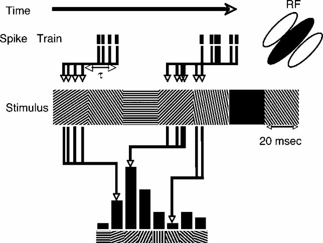
Figure 1. Schematic representation of reverse-correlation in orientation space. As time proceeds from left to right, spikes times are recorded (tick marks), in response to the random grating stimulus sequence. An example of a short segment of the stimulus is shown below – a new random orientation is presented every 20 ms. For a set value of τ a histogram of the stimulus orientation present τ ms before each spike is computed. The schematic RF of the neuron is oriented at 45 degrees, so the majority of spikes are in response to gratings oriented near 45 degrees.

The degree of orientation selectivity was defined as the orientation selectivity index (OSI) (Swindale, 1998 ), calculated as:

where R is average response during grating presentation and θ is orientation from 0 to 157.5, indexed by i = 1 to 8. The OSI is a continuous measure with values ranging from 0 (unselective) to 1 (perfectly selective).

From 111 single units isolated, 86 were selected for analysis because they met two criteria: response amplitude reached 150% of baseline amplitude and OSI reached three SDs above baseline levels. Simple and complex cells were differentiated based on the ratio of the magnitude of the F1 Fourier component of the response (the response component at the temporal frequency of the stimulus) to the F0 component (mean, or DC component of the response, Skottun et al., 1991 ).

Bayesian Model for Fitting Data

We used a generative Bayesian model to obtain a detailed description of the relationship between the oriented movie stimulus and the spiking response of each cell (Carlin et al., 2003 ; Sahani and Linden, 2003 ). This approach allowed us to determine whether the tuning curves are significantly different at different delays. We employed Markov chain Monte Carlo (MCMC) sampling techniques to estimate the distribution of the parameters of the model for each cell. The results of these MCMC sampling runs provide estimates of the expected values of the tuning curve parameters, as well as estimates of the remaining uncertainty

To model the orientation tuning of each cell, we assumed that the neuron's response at each moment in time following the presentation of a particular stimulus orientation can be characterized by a circular Gaussian (CG) tuning curve, where the parameters of this Gaussian curve change as a function of the time lag after stimulus presentation. Each CG can be completely described by four parameters: the baseline, amplitude, preferred orientation (mean), and tuning width (standard deviation). Because we bin the spike trains at 5 ms for this analysis, a total of 20 such curves would be needed to describe the response of the cell in the 100 ms following each stimulus frame. We further assumed that the CG parameters change smoothly over the time course of the neuron's response. This assumption is implemented as a “smoothness prior,” the particular form of which is described below.

The basic premise of the model is that each time a particular stimulus frame is presented, the firing rate of the neuron is modulated in a characteristic, time-lag-dependent way over the subsequent time window. The instantaneous firing rate of the cell is a summation of the influence of the preceding stimulus frames whose windows “cover” the current time point.

Formally, the model is completely characterized by a specification of the joint probability distribution of the model parameters and the observed data. This joint probability factorizes as follows:

The factors on the right-hand side of the above equation will be specified in turn. All symbols are explained in Table 1 .

1. Data likelihood: The orientation selectivity of the neuron at each 5 ms time bin after stimulus presentation is assumed to follow the form of a CG curve. That is,
   
   The maximum delay is a value chosen to be appropriate to the response window of each cell. The firing rate is the sum of all stimulus-induced spiking propensities that are currently active. The firing rate at time t is therefore calculated as:
   
   Here, the [·]₊ notation indicates that the firing rate is half-rectified in order to ensure that it is non-negative. The quantity is a deterministic function of the tuning curve parameters. Its realization as a random variable is therefore (trivially) formulated as:
   
   The likelihood of the observed spike train can then be evaluated directly from p(t), as a series of Poisson trials:
   
2. Tuning curve parameters: The distribution of the CG tuning curve parameters B, A, PO, TW, as well as the blank response Bl, are described below. The value of each of these parameters as a function of the lag τ is assumed to be characterized by a discrete-time random walk, whose step size is drawn from a zero-mean normal distribution. That is, . Furthermore, because the step sizes are independently drawn, the probability of observing a particular parameter time course is simply the product over Gaussian likelihoods:
   
3. Hyperprior parameters: The variances of the random walks are distributed as a scaled inverse Chi-squared random variable with T -1 degrees of freedom:
   
   This is one formulation of an “uninformative” prior over the variance of normally distributed data.
4. Inference and sampling. The goal of Bayesian inference is to describe the posterior distribution of the model parameters, given both the observed data and our prior knowledge about the distribution of these random variables. Using Bayes’ Rule and substituting the model described above, this posterior is as follows:
   
   We used MCMC sampling methods to obtain an approximation of the posterior distribution. In particular, we use Gibbs sampling to sample the values of the random walk parameters, and Metropolis sampling for the tuning curve parameters.

TABLE 1

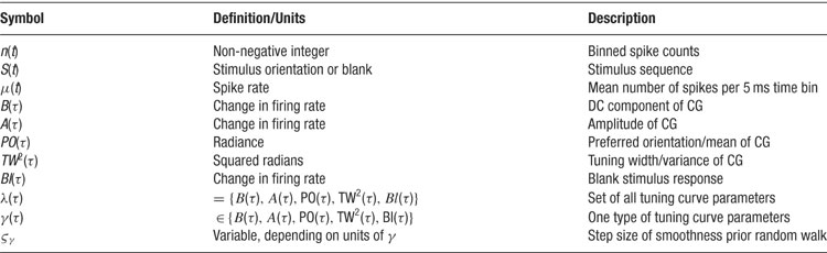
Table 1. Symbols and definitions used.

The distributions of the tuning curve parameters do not have a simple form, and we therefore turn to Metropolis sampling to infer their values. We use a jumping distribution which moves along directions in parameter space which correspond to individual components of the discrete cosine transform (DCT) of the previous sample. Briefly, the procedure is as follows. At each sampling step, we randomly choose one of the parameter types (B, A, PO, TW, or blank), and we calculate the DCT of this chosen parameter vector. We then choose one frequency at random, favoring the low-frequency components (which are the “smoothest”), and perturb this one frequency component by a small amount. Finally, we perform the inverse DCT to transform the parameter values back into the original space. The result is a proposed parameter time course which is smoothly deformed from the previous sample.

In practice, the Bayesian model was able to provide reasonable sampling results on the 70/86 cells for which 400 or more recorded spikes were available. Of these 70 cells with sufficient spikes, evidence for orientation tuning at some delay after stimulus onset could be reliably found in 58 cells (determined by checking whether the amplitude parameter of at least one of the CG tuning curves was significantly above it's “resting” value with a confidence level of 95%). The remaining 12 cells were either untuned, or (more likely) exhibited orientation-specific responses which were too noisy for the statistical model to reliably identify. In this regard, it is noteworthy that many of these 12 “inconclusive” cells exhibited low spike counts, which resulted in greater uncertainty about their response properties and correspondingly larger error margins in the sampling results.

Computational Model

Overview. We used a two–dimensional large-scale Hodgkin–Huxley network model to analyze response dynamics in relation to the orientation map. The model was based on a previous model (Mariño et al., 2005 ). We used a grid of 50 × 50 neurons for the excitatory layer and 1/3 × 50² neurons placed at random locations in the inhibitory layer. The model thus contained 75% excitatory and 25% inhibitory cells. All model cells received synaptic background activity, afferent and recurrent input from AMPA, NMDA, and GABA_A synapses. Cells were arranged in a two-dimensional grid, connecting to other cells according to a spatially isotropic connectivity profile. The afferent input to each cell was given by its location in an artificial orientation map consisting of four pinwheels (Kang et al., 2003 ; McLaughlin et al., 2000 ; Figure 9 A). Extending the model described in Mariño et al. (2005) , time-dependence of the input was introduced: an artificial reverse-correlation stimulus was created by generating a time series consisting of 20 ms blocks of one of 16 orientations or “blanks”. For each neuron, this stimulus was then filtered with a Gaussian orientation tuning curve according to the preferred orientation of the neuron. To capture the temporal characteristics of the inputs each cell received one out of four differently parameterized temporal kernels, which capture the variability present in LGN and V1 simple cell responses (Alonso et al., 2001 ; Wolfe and Palmer, 1998 , see Figure 9 B). Using this filtered input as a time-varying firing rate, 20 Poisson input spike trains were generated for each cell. The network was simulated for 250 s with 0.25 ms resolution. The spike output of the excitatory cells was then analyzed using the reverse-correlation technique described above.

Single cell description. The dynamics of the membrane potential V is described by

where I_syn and I_int denote the synaptic and the intrinsic voltage-dependent currents, g_L and E_L denote the leak conductance and its reversal potential, C_m denotes the membrane capacitance, and t the time (for parameters see Table 2 ).

TABLE 1

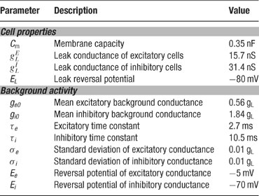
Table 2. Single cel properties.

Each current I_int is described by a Hodgkin–Huxley equation

where is the peak conductance, E is the reversal potential, and m(t) and h(t) are the activation and inactivation variables. We included three voltage dependent currents: a fast Na⁺ current and a delayed-rectifier K⁺ current for the generation of action potentials, and a slow non-inactivating K⁺ current responsible for spike frequency adaptation. These active conductances were modeled as described in Destexhe and Pare (1999) . The peak conductance of the non-inactivating K⁺-current is multiplied by the factor 0.1 for inhibitory neurons, thereby reducing the spike-frequency adaptation.

All model neurons received background synaptic inputs, described by an excitatory and an inhibitory background, conductance, each independently following a stochastic process similar to an Ornstein–Uhlenbeck process. The following update rule was used (Destexhe et al., 2001 ):

where g⁰ is the average conductance, τ is the background synaptic time constant, A is the amplitude coefficient and N(0,1) is a normally distributed random number with zero mean and unit standard deviation. The amplitude coefficient has the following analytic expression:

where D = 2σ²/τ is the diffusion coefficient.

Numerical values for the background conductances are given in Table 2 .

Synaptic input. Each neuron receives recurrent excitatory input from N_e = 100 and recurrent inhibitory input from N_i = 50 neurons. All recurrent connections to a given neuron were sampled based on a rotationally symmetric Gaussian probability distribution:

where x is the distance in pixels and σ = 4 pixels (corresponding to σ = 125 μm).

The synaptic currents I_syn were then computed using the following equation:

where g_j and E_j are the time-dependent conductance and the reversal potential for the j-th synapse, and is a scale factor (for values see Table 3 ). We distinguish between an inhibitory GABA_A-like, a fast AMPA-like excitatory and a slow NMDA-like excitatory component for recurrent synaptic connections. The total excitatory postsynaptic potential is hence the sum of a fast and a slow component with the time-integrated contribution of each component being 70% and 30% respectively. The dynamics of the fast excitatory and of the inhibitory synaptic conductances are described by (Destexhe et al., 1998 )

where τ_j is the time-constant of the j-th synapse, and where the presynaptic spike train with spike times is described by the sum of δ-functions. The dynamics of the NMDA-like component is given by (Destexhe et al., 1998 )

with time constants τ₁ = 80 ms and τ₂ = 2 ms.

TABLE 3

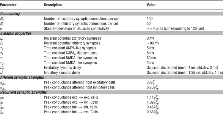
Table 3. Parameters for connectivity and synapses.

The for an individual synapse was determined by normalizing the values with respect to the number of synapses of the corresponding type connected to the neuron.

Afferent input. Each neuron receives afferent input from N_Aff = 20 excitatory synapses. This feedforward input consists of Poisson spike trains generated from a time varying firing rate f_Aff. For a cell c, this firing rate is given by

where θ(t) is the presented orientation at time t, r_c is the orientation tuning curve, and h_c is the temporal response envelope of cell c. The response r_c as a function of stimulus orientation is given by a Gaussian distribution added to a baseline

where θ_c is the preferred orientation of the neuron c (chosen according to the artificial orientation map shown in Figure 9 A), σ = 27.5° is the orientation tuning width, and r_base = 0.1 is the baseline response. For each cell, one of four temporal kernels h₁… h₄ was chosen with probability 0.3, 0.3, 0.2, and 0.2, respectively. This randomness in the temporal input characteristics modeled the variability observed in the temporal responses of LGN and V1 simple cells in cat (Alonso et al., 2001 ; Wolfe and Palmer, 1998 ). The four kernels were all modeled as Gamma functions multiplied with a cosine, a description that has been shown to generate temporal profiles closely resembling those of V1 simple cells (Chen et al., 2001 ):

where Γ(a) is the standard gamma function. The parameters we used for the temporal kernels are summarized in Table 4 (see also Figure 9 B). Each kernel was scaled such that, if the neurons were driven by afferent input of that kernel alone, this neuron would fire at 6 Hz for the preferred orientation stimulus. In the simulations with more uniform afferent input (Figure 9 D), the temporal kernels were assigned randomly to the individual afferent input synapses instead of assigning one temporal kernel to all synapses of a given cell. Therefore, each cell received input from afferent synapses with different temporal behavior. This had the effect of making the effective afferent input time course more similar across cells.

TABLE 4

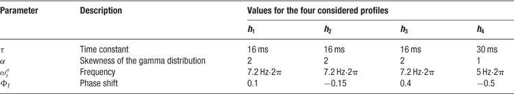
Table 4. Parameters for the temporal input kernels.

Results

To examine the dynamics of orientation selectivity in V1, RFs were stimulated with a dynamic grating sequence protocol similar to those in previously published reports (Ringach et al., 1997a ; Ringach et al., 1997b ). The spike times were reverse-correlated with the stimulus sequence to estimate the linear relationship between stimulus orientation and firing probability. Summing over all spikes, the probability distribution of stimulus orientation occurring τ ms before the occurrence of a spike was generated. The relative probability of different orientations eliciting spikes as a function of time was estimated over a series of τs. In this paper, we will refer to these probability distribution functions simply as orientation tuning curves.

Evolution of the Orientation Tuning Curve

We first describe the basic features of the tuning curves and their changes over time. Tuning curves were calculated at τs ranging from -20 ms (before stimulus onset), up to times exceeding the response duration (150 ms), in steps of 1–10 ms. Many of the basic features of the responses in our population of cat V1 neurons were similar to those previously reported using similar protocols in macaque monkey V1 neurons (Dragoi et al., 2002 ; Mazer et al., 2002 ; Ringach et al., 1997a ; Ringach et al., 1997b ). As expected, the tuning curves at τs <25 ms were generally flat, indicating that the stimulus had not yet influenced the firing probability of the neuron. Beginning at τs between 25 and 50 ms, orientation selectivity began to emerge.

Figure 2 shows the timecourse of responses for a typical cell. Panel A depicts the tuning curves at τs ranging from 0 at the bottom to 110 ms at the top. For τ < 30 ms, the tuning curve is flat. At 30 ms, tuning begins to emerge, and peak amplitude of the tuning curve is reached at 50 ms. Thereafter, the tuning curve gradually becomes flatter, until it is almost flat at 110 ms. The tuning width is fairly constant at all τs, but the amplitude and the offset change over the course of the response. Panel B shows the response for each orientation individually. In these plots, which depict the impulse response, or the height of the tuning curve bin for one orientation as a function of time, the response to each orientation can be seen more clearly. This type of display is analogous to the peri-stimulus time histogram, typically used to display steady-state responses to flashed stimuli, and we therefore refer to them as PSTH plots. The response to the preferred orientation (90 degree) begins at 30 ms, peaks at 50 ms, and then decays back to zero in two stages. The response to the orthogonal orientation is very small, but shows a small initial positive response, followed by a small negative dip.

FIGURE 2

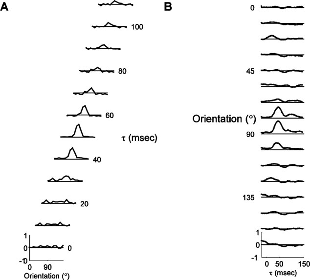
Figure 2. Example of orientation dynamics. (A). A series of tuning curves taken at τs ranging between 15 and 125 ms after stimulus onset, as indicated to the right of each plot. The height of the tuning curves at each orientation represents the normalized probability that a spike was fired, plotted between -1 and 1, as indicated by the scale for the bottom curve. The solid line represents zero. (B). The timecourse of response for each orientation, from τ = -20 to τ = 145. The vertical scale and the position of the reference lines are identical to those in panel A.

Across the population of cells recorded (n = 86), the time of the first significantly selective tuning curve was 34.3 ± 4.3 ms (Figure 3 ). The time of peak response amplitude was 55.8 ± 3.2 ms. In general, the temporal profile of selectivity was similar across the population (Sahani and Linden, 2003 ); the selectivity increased rapidly after onset, peaked for a short period of time (<10 ms), and then decayed back to a flat, untuned curve. The largest variability in timing came during the declining phase of the response (τs greater than ∼60 ms). Some neurons were only selective for short durations (<30 ms), whereas others continued to be selective for τs up to 150 ms. The diversity of decay dynamics is apparent in the spread of the distribution of τ_dec, the time point at which the response to the preferred orientation has relaxed to half the peak value (Figure 3 C).

FIGURE 3

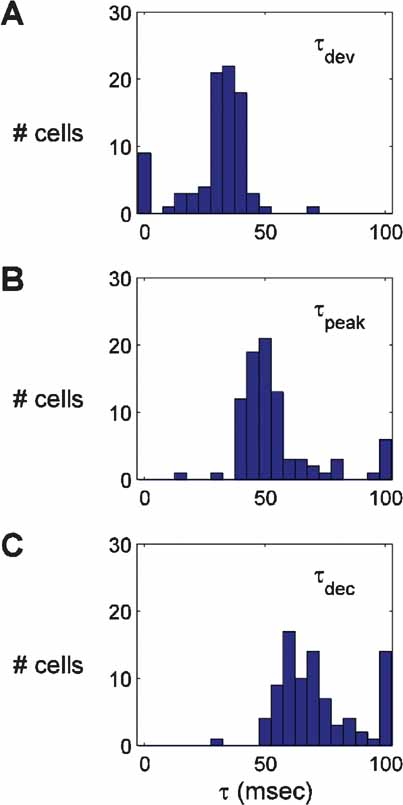
Figure 3. Histograms of three indices of the timecourse of responses. The middle panel shows the time of peak response (τ_peak). The top panel shows the timepoint τ_dev, at which the response is half the amplitude reached at τ_peak. The bottom panel shows the time point τ_dec after the peak at which the tuning curve amplitude has fallen to half of the peak value.

Tuning Curve Stability

We next assessed the degree of stability of tuning curves as a function of time during the response. One of the difficulties in judging stability of tuning curves is to determine the confidence (or conversely uncertainty) in parameters of the tuning curves extracted from repeated presentations of the same stimulus. To address this issue, we have used a generative Bayesian model to define confidence bounds on the tuning curve parameters at each τ, under the assumptions of a Gaussian tuning curve, and smooth changes in tuning curve parameters with time. This model has the advantage that probabilities are assigned to all combinations of tuning curve parameters, and thus the likelihoods of different tuning curves at each τ (e. g. the probability of a shift versus. no shift in preferred orientation) can be directly compared. Figure 4 A–4 D shows an example of a cell that showed no significant changes in tuning width or preferred orientation. The confidence bounds overlap throughout the entire response, thus not indicating any significant change in either parameter. Intuitively, this can be readily visualized: the parameter does not change because a horizontal line would fall within the confidence bounds at all τs. In another example in Figure 4 (Cell 2; Figure 4 E–4 H), this is not the case. There is no horizontal line that could be contained within the confidence bounds for preferred orientation (Figure 4 G); therefore, we can say with confidence that the preferred orientation changes between τ = 60 and 70 msec. Likewise, it is clear that the tuning width of Cell 3 decreases significantly (Figure 4 L).

FIGURE 4

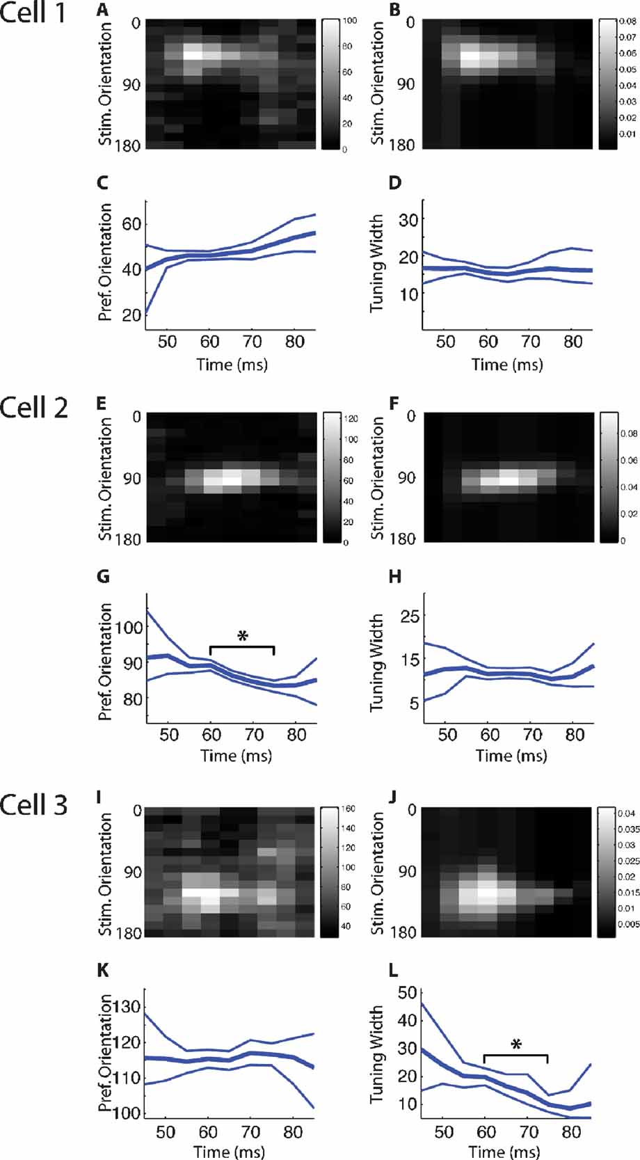
Figure 4. Bayesian model fitting results for three example cells. A–D. Results from a cell which does not show evidence for a shift in either preferred orientation or tuning width. (A) The stimulus-triggered average response of the cell to stimuli of different orientations. The values shown indicate the total number of spikes which were observed to follow each stimulus orientation by a particular time lag (binned at 5 ms). (B) The expected response of the cell, as a function of stimulus orientation and time lag, as estimated by the Bayesian model fitting procedure. Plotted values indicate the estimated change in firing rate that is induced by each stimulus orientation at a particular time lag. (C) The time course of the preferred orientation parameter of the Bayesian model, showing the expected value (thick line) and 95% error margins (thin lines). (D) The time course of the tuning width parameter of the Bayesian model, again showing the expected value and 95% error margins at each time lag. (E-H) A cell which undergoes a shift in preferred orientation (in G) over the time course of its response; conventions as in (A-D). (I-L) A cell which sharpens its tuning (in L) over the time course of its response; conventions as in (A-D).

With this approach we determined that a substantial number of cells show statistically significant changes in tuning curve parameters over a period of the response between the peak of the response, and τs later in the response. Twenty-six percent (15/58) of cells showed a significant shift in preferred orientation. The mean size of these shifts was 12 degrees, with a standard deviation of 6 degrees; the largest observed shift was 24 degrees. Seventeen percent of cells (10/58) showed a sharpening of tuning, and 7% (4/58) showed a broadening. When observed, these changes in tuning width typically continued to increase in magnitude throughout the later portion of the response (as in the example cells in Figure 4 ). The mean magnitude of the tuning width changes (including both broadening and sharpening) was 12 degrees, with a standard deviation of 6 degrees. Overall, 38% (22/58) of cells showed some significant change in tuning curve parameters. Thus, a substantial minority of cells showed significant changes in either tuning width, preferred orientation, or both. The changes were typically small, but reliable, indicating that subtly different inputs during different phases of the responses can be reliably detected with our stimulation protocol and analysis tools.

Comparison of Simple and Complex Cells

Two main classes of RFs have been described in V1 neurons: simple and complex. The two types are distinguished largely by the linearity of their spatial transformation of visual input to spiking response (Hubel and Wiesel, 1962 ; Movshon et al., 1978 ; Skottun et al., 1991 ). Figure 5 shows the average timecourse of the OSI for the populations of simple and complex cells. The timecourses differ in three aspects. First, simple cells are more selective, seen as a higher peak OSI, as is found using standard steady state recordings (Heggelund and Albus, 1978 ; Leventhal and Hirsch, 1978 ; Ringach et al., 2002 ). Second, the time of peak OSI is earlier for simple cells (44 vs. 54 ms). Third, the baseline OSI is higher for simple cells. Otherwise, the evolution of selectivity is similar between the two cell classes. The earlier peak in selectivity of simple cells is consistent with the hierarchical description of information flow through V1: simple cells predominate at the input stages of V1 whereas complex cells are in the majority at later stages. There is a wealth of anatomical and physiological data supporting this arrangement (Alonso and Martinez, 1998 ; Ferster and Lindstrom, 1983 ; Gilbert, 1977 ; Martin and Whitteridge, 1984 ).

FIGURE 5

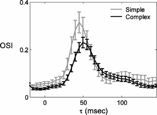
Figure 5. Comparison of the timecourse of selectivity in simple and complex cells. (A) The average ± SEM of the OSI is plotted as a function of τ for the population of simple (n = 26) and complex cells (n = 60).

Dependence on Cortical Depth

Inputs from the LGN impinge mostly in layer IV, but also project to layer VI and lower layer III (Douglas and Martin, 1991 ; Ferster and Lindstrom, 1983 ; Humphrey et al., 1985 ). Layer IV neurons, in turn, send strong projections to the superficial layers, which send strong projections deeper layers (Gilbert and Wiesel, 1979 ). It is therefore to be expected that the timecourse of responses might be subtly different in the different cortical layers, due to the synaptic latencies at each stage of the circuit. To test whether reverse-correlation can discern these different “stages” of visual processing, and whether orientation dynamics are layer specific, the dynamics of tuning properties were analyzed separately for different layers. Due to the uncertainty of the exact laminar position of our recording sites, this was done by pooling those neurons estimated to be in the supragranular layers (<600 μm), the middle layers (600–1200 μm) and the infragranular layers (>1200 μm). The assignment to laminar groups is corroborated by an analysis of the F1/F0 ratio as a function of depth; the highest ratio of simple cells is found between 600 and 1200 μm, providing support for the assignment of laminar location on the basis of microdrive depth readings (data not shown).

Figure 6 shows the average tuning curves and timecourses from the three laminar groups. Figure 6 A shows the tuning curves at a series of τs, and Figure 6 B shows the PSTH plots for each orientation. As expected, several subtle patterns can be discerned. First, the time of peak response is slightly earlier for cells in the middle layers than for the superficial and deep neurons. Second, the responses of middle layer neurons are slightly shorter, the responses of deep layer neurons are substantially longer, and the responses of superficial layer neurons are intermediate in duration. The median peak time for middle layers is 45.5 ms, 7.5 ms earlier than the median peak time for the superficial group, and 5.5 ms earlier than for the deep layers. These differences can be seen more clearly in the expanded plots of the responses to the preferred and orthogonal orientations (Figure 6 C and 9 D). The intermediate peak time for the deep layers is most likely because it comprises a mixture of layer VI, which receives direct LGN input, and layer V, which only receives multi-synaptic inputs from the LGN. The response decay is also different in the different layers, with the middle layers falling off the fastest followed by the superficial and then the deep layers. Thus, the reverse-correlation procedure is capable of resolving small timing differences between neurons in different laminae.

FIGURE 6

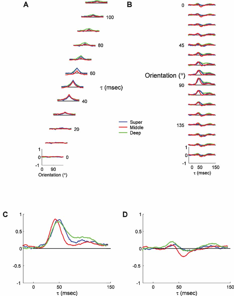
Figure 6. Average dynamics of tuning as a function of laminar position. (A) Average tuning curves of neurons recorded in superficial layers (<600 μm; n = 18), middle layers (600–1200 μm; n = 40) and deep layers (>1200 μm; n = 28). The scaling and conventions are the same as in Figure 2. Lines representing ±2 SDs have been omitted for clarity. (B) The timecourse of responses for the three laminar groups plotted in panel A. (C) Expanded view of the PSTH plot of the responses to the preferred orientation (90 degrees), to highlight the differences between the different laminar groups. (D) Expanded view of the PSTH plot of the responses to the orthogonal orientation (0 degrees).

Other than these differences in the timing of responses, the overall tuning characteristics of all three groups are fairly similar. The tuning widths, the OSI and the general tuning curve shape are nearly indistinguishable for the three groups. There is no evidence of substantial changes in the tuning curve shape over time for any of the laminar groups. Suppression at the orthogonal orientation is slightly earlier and larger in the middle layers than in the other two groups (Figure 6 D). The timing difference is consistent with overall faster responses resulting from strong direct thalamocortical projections to middle layer neurons. The larger size of suppression could reflect the strong inhibition that both feedforward and recurrent models find to be necessary to suppress thalamocortical inputs at orthogonal orientations. Overall, the analysis of orientation dynamics at different cortical depths is consistent with known differences in the circuitry.

Dependence on Location Within the Orientation Map

We also tested the hypothesis that neurons situated near pinwheel centers in the map of orientation preference have different dynamics than neurons far from pinwheel centers. Neurons near pinwheel centers receive intracortical inputs from a wider range of orientations (Schummers et al., 2002 ; Yousef et al., 2001 ) than neurons in the center of orientation domains. Tuning curves of pinwheel center and orientation domain neurons were analyzed separately to determine if any features of the tuning curves reveal the different inputs they receive. Figure 7 A shows the average tuning curves of the two populations over the timecourse of the response. The tuning curves demonstrate, as with previous measurements of steady state responses (Dragoi et al., 2001 ; Maldonado et al., 1997 ; Schummers et al., 2002 ), that cells have equally sharp tuning at pinwheel and orientation domain locations. Furthermore, there is no evidence of instability, shifts, multiple peaks, or any other gross differences in tuning in the cells near pinwheel centers. For all τs up to 45 ms, the average tuning curves of the two populations are nearly indistinguishable. The first small difference is that the peak of the tuning curve for orientation domain neurons is slightly higher at τ = 45. This is seen more clearly in the PSTH plots shown in Figure 7 B. Given the normalization procedure applied to these plots, the explanation for this difference is that there is more spread in the time of the peak response in pinwheel neurons. Since each neuron is normalized to the maximum response at any τ, if all neurons peaked at the same time, the peak of the average plot would be one. Thus, the difference in the amplitude of the peak response is indicative of a spread in peak time, rather than a difference in response magnitude. This suggests that there is more spread in the timing of responses in the population of neurons in the pinwheel group.

FIGURE 7

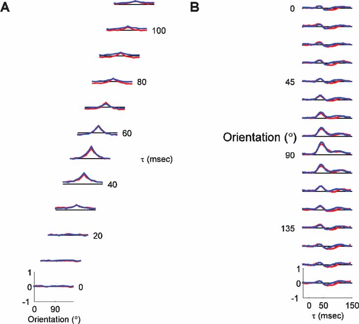
Figure 7. Orientation dynamics for pinwheel center and orientation domain neurons. (A) For each τ, the average tuning curve for all the pinwheel neurons (red; n = 31) and orientation domain neurons (blue; n = 55) is plotted. The vertical scale is the same for all τs. The tuning curves represent the average of normalized individual tuning curves, with zero representing the blank response, and 1 representing the maximal response at all τs and orientations. The dashed black line represents the response to the blank stimulus for each τ. Thus, points in the tuning curve above the dashed line indicate enhancement of firing, whereas points below the dashed line represent suppression of firing. (B) Average PSTH plots for pinwheel and orientation domain cells.

To explore this possibility in more detail, we examined the timecourse of responses for each cell individually. Figure 8 plots the PSTH plot for the preferred orientation of each orientation domain cell (left) and each pinwheel cell (right). It is clear from visual inspection of these plots that there is indeed more variability in the timing of responses in the population of pinwheel neurons. This impression is confirmed by a quantification of the variance as a function of time in the population of cells in the pinwheel and orientation domain groups. Figure 8 B plots the timecourse of variance for pinwheel (red) and domain (blue) cells for each stimulus orientation. For the preferred orientation, higher variance in the pinwheel population was most prominently following the peak response, during the decay phase. For all orientations, the variance was higher in pinwheel cells for the entire response duration, particularly after the peak of the response. This suggests that the timing in orientation domain cells is much more uniform, while the timing of pinwheel center cells is much more heterogeneous. To examine the possibility that the differences in the timing of pinwheel and domain responses are due simply to differences in the distributions of laminar position in the two groups, we plotted the differences in timing for each layer independently. Figure 8 C shows the timecourse of the response to the preferred orientation as a function of map location (columns), and laminar position (rows). There is more variability in pinwheel neurons in all three layers. Despite this variability, the main laminar differences of earlier peak time in middle layers, and prolonged response in deep layers are apparent in both pinwheel and domain populations. Thus, laminar position seems to determine the average timing of responses, and map location influences the variability of response timing about these means. These analyses suggest that despite having similar mean population tuning curves, there is substantially more individual variability in the timing of enhancement and suppression that shape the tuning curves of pinwheel cells. One potential explanation for this effect is the local cortical network surrounding the sites classified as pinwheel center, which are more heterogeneous than those in orientation domains (Mariño et al., 2005 ).

FIGURE 8

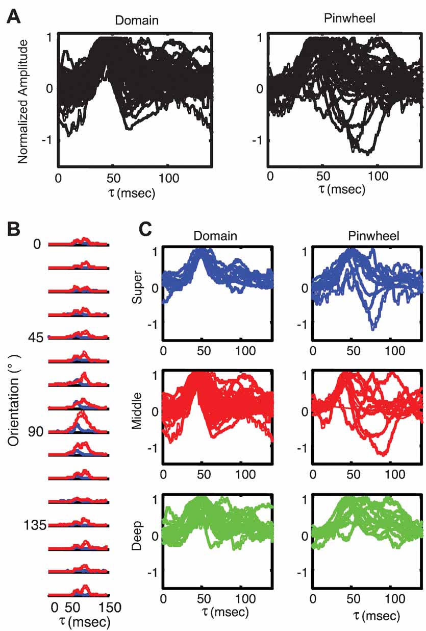
Figure 8. Response timing is more variable near pinwheel centers. (A) PSTH plots of responses to preferred orientation of individual orientation domain neurons (left; n = 55) and pinwheel center neurons (right; n = 31). (B) Plots of population variance in response amplitude as a function of time for each stimulus orientation. Pinwheel neurons are plotted in red and orientation domain neurons in blue. (C) PSTH plots of individual neurons, grouped as a function of laminar position and orientation map position. Orientation domain cells are plotted in the left column, and pinwheel center neurons in the right column. Superficial layer cells are plotted in blue in the top row, middle layer cells are plotted in red in the middle row and deep layer cells are plotted in green in the bottom row.

Modeling the Differential Response Signatures Close to Pinwheels and in the Orientation Domain

To elucidate the mechanisms behind the observation that pinwheel cells show similar average response dynamics but have much higher variability than their orientation domain counterparts, we simulated a large-scale neural network of a patch of V1 containing four pinwheel centers (Figure 9 A). To realistically model the timecourse of visual responses, the inputs to the model were filtered using temporal kernels matched to the impulse response functions of LGN cells (Figure 9 B). The strength of the recurrent connections was chosen such that excitation and inhibition were balanced with one another and provide significant input to the model neurons, as is necessary to account for the subthreshold membrane potential and conductance tuning in pinwheel and orientation domain neurons (Mariño et al., 2005 ).

FIGURE 9

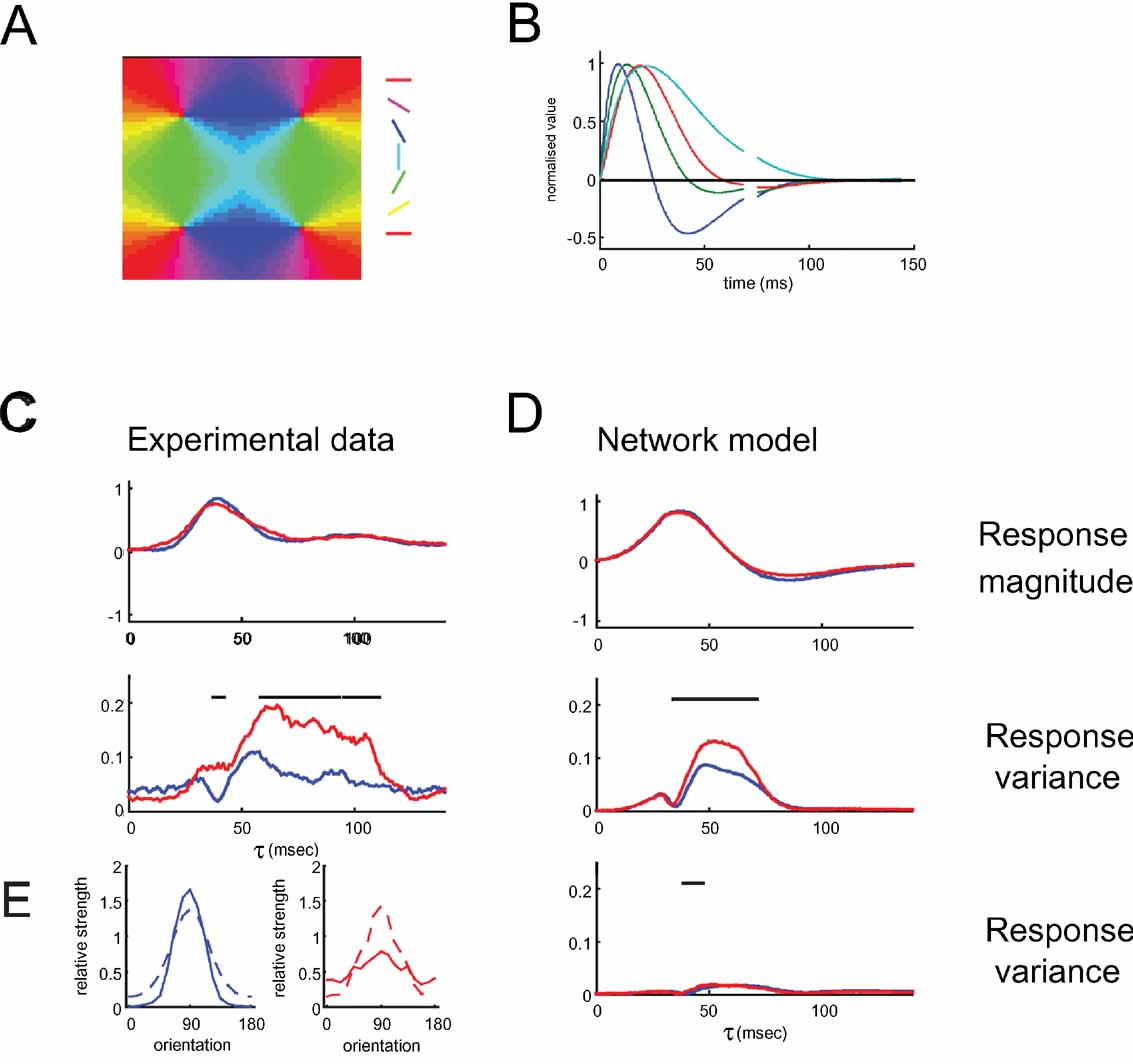
Figure 9. Mean temporal response and variance of response timing in the network model of pinwheel and orientation domain cells. (A) The artificial orientation map used in the model. (B) Temporal kernels of inputs to the model neurons. See Methods for details. (C) Experimental data. The mean temporal response (top) and variance (bottom) across cells is plotted in red for pinwheel neurons and in blue for orientation domain neurons. (D) Plots of mean temporal response (top) and variance (middle) in response to preferred orientation for the network model. Experimental data and model responses both have similar mean temporal response of pinwheel and orientation domain cells. In the late part of the response, the variance in the time course of pinwheel cells is significantly higher than in orientation domain cells. The bottom panel shows the variance for the same model network, if individual neurons all received as input a similar mix of the different afferent cell types (i.e. temporal kernels). Note that in this case, the variance is much lower and there is no difference in the variance for pinwheel and orientation domain cells. Black lines on top of the figures indicate significantly higher variance in pinwheel neurons compared to orientation domain neurons. Significance was assessed using a bootstrap method, randomly choosing 50 pinwheel and 50 orientation domain neurons to compute and compare the variance pinwheel and orientation domain neurons’ responses for each time lag τ, repeating this procedure 1000 times to estimate the probability of the variance of pinwheel neurons being larger than that of orientation domain neurons, regarding it significant above 95%. For the experimental data, we applied the same method, sampling a subset of 15 pinwheel and 15 orientation domain neurons at each repetition. E. Tuning of the excitatory conductances of orientation domain neurons (left panel, blue) and pinwheel neurons (right panel, red). The afferent input (dotted lines) has the same strength for both, pinwheel and orientation domain cells. For the preferred orientation, the strength of the total recurrent excitatory conductance (solid lines) is higher in orientation domain neurons. For this analysis, the network received time-invariant input, simulating a constant visual stimulation with a single orientation.

The timecourse of the activity of the model neurons captures the onset and the phasic part of the neuronal responses well (Figure 9 C and 9 D, top). The decay phase is less well described: the real neurons show a small second peak (100 ms) and a plateau of sustained activity following their initial decline; the model neurons, on the other hand, decline further to below baseline. Nevertheless, as in the real neurons, throughout the whole timecourse, the average responses of pinwheel and orientation domain neurons are similar. This is despite the fact that cells close to a pinwheel center receive recurrent input from cells with a much broader range of preferred orientations. However, the difference in the local circuitry does have an effect on the variance of the neuronal responses: the variance of the pinwheel cell responses in the model is larger than that in the orientation domain (Figure 9 D, middle), which is in fact, like for the experimental data, true for all orientations (data not shown). Unlike for the real neurons, this larger variance in pinwheel neuron responses can be seen in the model only up to 90 ms after stimulus onset.

Thus, the model is able to capture the main features of the responses of the real neurons with the exception of the late part of the response. The suppression of the model neurons following the phasic part of the response can be linked to the spike-frequency adaptation in the model; removal of this feature does not, however, produce the second response peak, observed in the real data (not shown). Thus, the discrepancy between model and real neurons during the late phase of the response is likely to be found in the models simplicity; because of its restriction to the local recurrent network it does not incorporate any long-range horizontal and feedback connectivity, which may cause sustained activation of the neurons. Alternative explanations, such as global oscillatory behavior of cortex in response to the flashed grating stimulation are also difficult to reproduce in a simple one-layered network. Despite the simplicity of the model, the responses of model and real neurons are in good qualitative agreement during the first 90 ms.

The more variable responses of the pinwheel neurons may appear trivial at first glance, since the recurrent inputs to the pinwheel cells are less uniform. However, on closer inspection we find that rather than having the non-uniform recurrent connections of the pinwheel cells introducing variability into their responses, what actually happens is that the more uniform responses of orientation domain cells provide smoothing of the temporal variability already present in the input to the V1 cells. This can be seen in simulations where all network neurons received similar input: all cells then did in fact show smaller variance in their responses, and the difference between pinwheel and domain disappears (Figure 9 D, bottom).

The cause of the differential smoothing effect in pinwheel and orientation domain can be observed directly by assessing the mean excitatory input conductances received from the different sources by pinwheel and orientation domain neurons as a function of stimulated orientation (Figure 9 E). The relative contribution of feedforward connections to a cell's inputs of the preferred orientation is far greater in the pinwheel than in the orientation domain. This means that the afferent input drives pinwheel neurons more effectively than orientation domain neurons, which receive strong recurrent excitation. Thus, any variance present in this feedforward input will have a more dominant effect on the cells response.

Factors other than the uniform afferent input can also be seen to alleviate the location dependence of the response variance. In particular, parameters which slow down the responsiveness of the network (like increasing the proportion of NMDA synapses) result in a decrease of the difference between pinwheel and orientation domain neurons. This is intuitive: NMDA synapses have time constants of a magnitude similar to the pulse-length received from the slowest population of afferent inputs. Thus, they effectively prolong the fast afferent inputs, making them more similar to one another.

One may hypothesize that other parameter manipulations may also result in the variance differences between pinwheel and orientation domain neurons, not requiring the variability to be present in the afferent input already. However, parameter changes, which may appear well-suited for introducing more variance into pinwheel neurons, such as varying the afferent input strength for different model cells or using a less symmetric orientation map for assigning the preferred orientation of the afferent inputs, did not lead to larger variance in the pinwheel neurons (data not shown). Thus, the temporally variable afferent input appears essential to reproducing the behavior of the real neurons in the model.

Taken together, the network model with balanced excitation and inhibition was able to reproduce both, the observed similar timecourse and different variability of the responses of cells near and far from pinwheel centers. The results indicate variability already present in the afferent input as a likely cause of the variability in pinwheel neurons.

Discussion

We have investigated the influence of local circuit constitution on the dynamics of orientation tuning in cat V1. While the general features of response timing in our data are similar to those previously reported, we do find that a large proportion of cells showing clear changes in tuning curve parameters during the response. We looked for subtle differences in response timing which reflect known differences in the inputs to different circuit locations. We found differences in timing in different cortical layers, and between simple and complex cells, all consistent with the known circuitry. We have also found that while the average timecourse of responses is similar in orientation domains and pinwheel centers, there is much more variability in the timing at pinwheel centers. Using a realistic, large scale model incorporating orientation map topology, we demonstrated that this previously unreported phenomenon is the natural result of a regime with balanced excitation and inhibition receiving LGN inputs with diverse temporal kernels.

General Features of Orientation Tuning Dynamics

The general features of the timing of tuning are similar in many respects to previous analyses of reverse correlation with dynamic grating stimuli from both cats and monkeys (Chen et al., 2005 ; Dragoi et al., 2002 ; Gillespie et al., 2001 ; Mazer et al., 2002 ; Nishimoto et al., 2005 ; Ringach et al., 2003 ). Previous studies have differed in whether they found changes in tuning curve parameters over the course of the response. Several studies of orientation tuning dynamics have noted large changes in either preferred orientation or tuning width (Chen et al., 2005 ; Ringach et al., 1997a ; Sharon and Grinvald, 2002 ; Shevelev et al., 1993 ; Volgushev et al., 1995 ), whereas several others have found stable tuning curve parameters (Celebrini et al., 1993 ; Dragoi et al., 2002 ; Gillespie et al., 2001 ; Mazer et al., 2002 ; Nishimoto et al., 2005 ). Using sophisticated Bayesian analysis, we demonstrated that in fact both phenomena occur in cat V1, with a large minority of cells showing significant, albeit small, changes in either tuning width or preferred orientation.

Influence of Cell Class and Laminar Position

The dynamics of orientation selectivity revealed differences in the time to peak selectivity between simple and complex cells. The most likely explanation for this finding is that simple cells receive strong direct thalamic inputs, whereas the majority of the drive to complex cells is at least one synapse removed from direct thalamic input. This is not surprising given that anatomical and cross-correlation studies have provided strong support for such an arrangement (Alonso and Martinez, 1998 ; Douglas and Martin, 1991 ).

The inputs to, and intrinsic connections within, different cortical layers are stereotypically different (Douglas and Martin, 1991 ). Direct inputs from LGN relay cells are limited to layers IV, VI, and lower layer III. Visually driven inputs to neurons outside of these layers are therefore necessarily delayed by at least one synapse, relative to the input layers. The exact laminar positions of the neurons recorded were not histologically reconstructed, but laminar location could be reasonably approximated by the depth readings of the microdrive. The accuracy of this method is corroborated by the higher probability of finding simple cells between 600 and 1200 μm. The grouping used here was chosen such that the “superficial” neurons were generally above the extent of LGN arbors, and therefore not thalamically driven, the “middle” neurons were likely to be within the reach of the main LGN arbors that target layer IV, and the “deep” neurons were likely to be below this main LGN projection zone, but may have received some direct projections via collateral projections to layer VI. Although these groupings are necessarily rough approximations, the differences in response timing among the groups bear out the accuracy of the estimates.

The major difference found between neurons in different layers is the timing of responses. Neurons in the middle layers on average had peak responses several milliseconds before those in the superficial or deep layers. The duration of responses was also shorter in the middle layers, and substantially longer in the deep layers. These differences are broadly consistent with the degree of thalamic input to the different layers; i.e., neurons in layers with more thalamic input respond faster. Of course, there are laminar differences in the proportions of simple and complex cells; unfortunately, the number of cells recorded does not allow a robust analysis of cell types in different layers. Regardless, the conclusion that more thalamic drive results in faster responses appears to hold. Together, these analyses demonstrate that different patterns of synaptic inputs to different cortical compartments have clear signatures in the dynamics of orientation tuning.

Orientation Dynamics Relative to Location in the Orientation Map

The similar degree of orientation selectivity in pinwheel center neurons and orientation domain neurons is consistent with previous studies of steady state orientation tuning that have also found no difference in firing rate tuning curves near pinwheel centers (Dragoi et al., 2001 ; Maldonado et al., 1997 ; Schummers et al., 2002 ). Previous studies have suggested that neurons near pinwheel centers receive subthreshold inputs at all orientations (Schummers et al., 2002 ). It might therefore have been expected that due to the continuous stimulation during the reverse-correlation stimulus protocol, neurons would be constantly depolarized and otherwise subthreshold inputs would be elevated above threshold, leading to broader tuning in this stimulus regime. Our results suggest, though, that the filtering of inputs at non-optimal orientations occurs prior to spike generation, regardless of the constant synaptic bombardment induced by the flashed grating stimulus. This is particularly important for neurons near pinwheel centers, where inhibition is critically required to balance strong excitation at non-preferred orientations (Mariño et al., 2005 ; Schummers et al., 2002 ). We have previously shown that the tuning of inhibitory conductances in pinwheel center neurons is nearly identical to the excitatory conductances (Mariño et al., 2005 ). This balance of excitation and inhibition ensures that suprathreshold tuning remains sharp even in the face of continuous visually-evoked inputs.

The higher variability in response timing near pinwheel centers probably reflects difference in the local cortical circuits at those sites compared to orientation domains. There is evidence that the local circuit connectivity is isotropic in V1, and thus, in orientation domains, local inputs are integrated from a patch of cortex that contains a representation of only a narrow range of orientations. All cells classified as orientation domain cells have a similar pattern of local inputs arising from neurons with a narrow range of preferred orientations. By contrast, the circuits near pinwheel centers are considerably more varied (Mariño et al., 2005 ; Schummers et al., 2004 ; Schummers et al., 2002 ; Yousef et al., 2001 ). In the network model, we implemented such a pattern of local recurrent connectivity, and in our simulations, we were able to confirm that this higher variability can reproduce the observed larger response variability near pinwheel centers. Since the network's input is matched to the output of LGN neurons, strictly speaking the model only represents something akin to the input layers of V1. However, the basic result easily be extended to other layers of V1. These, too, will receive strong visually driven input, likely originating in V1 simple cells. Such quasi-afferent input mediated through layer IV simple cells—while in timecourse shifted compared to LGN—nonetheless are very similar in their temporal characteristics to those of LGN cells (Alonso et al., 2001 ; Wolfe and Palmer, 1998 ). Thus, the results regarding similar timecourses in pinwheel and orientation domain as well as regarding differential variance generalize.

It is worth noting that the circuit variability alone is not sufficient to account for the differential output variability. Rather than actually introducing this variability through variability in pinwheel cells’ connectivity, the uniform recurrent connectivity in the orientation domain removes variability by integrating over the different inputs of their neighbors. This ability is reflected in the fact that the relative contribution of feedforward connections to a cell's inputs of the preferred orientation is larger for pinwheel cells than for orientation domain cells. The variability in the temporal response properties is already present in the responses of LGN neurons (Alonso et al., 2001 ; Wolfe and Palmer, 1998 ) and remains present in the input receiving (simple) cells of V1 (ibid.). The recurrent connectivity of V1 thus not only provides a shift-invariant representation in the complex cells (Shams and von der Malsburg, 2002 ), but also appears to provide a representation that is uniform in its temporal dynamics.

In sum, we demonstrate that reverse correlation analysis can detect subtle differences in neuronal responses that reflect their differential position in the local circuitry of cortex. Besides the known response differences detected, we also provide evidence for differing variability of the responses depending on location in the orientation preference map. We were able to demonstrate that this differential variability is consistent with a strongly recurrent network with balanced contributions of recurrent excitation and inhibition. Such a network has previously been implicated as prerequisite to account for orientation tuning observed in visual cortex (Mariño et al., 2005 ). Together, these studies highlight the importance of knowledge about the local network connectivity in understanding and modeling the orientation tuning in visual cortex.

Conflict of Interest Statement

The authors declare that the research was conducted in the absence of any commercial or financial relationships that could be construed as a potential conflict of interest.

Acknowledgements

This work was supported by NIH grants EY07023 and EY015087 (to MSu), and the BMBF under grant no. 01GQ0414 (KW, MSt, RM, and KO).

Author Contributions: J.S. and M.Su. conceived the experiment. J.S. conducted the experiments and much of the data analysis. B.C., K.K. conceived and implemented the analysis using the Bayesian model. K.W., M.S., R.M. and K.O. conceived and conducted the computational modeling work.

References

Alonso, J. M., and Martinez, L. M. (1998) Functional connectivity between simple cells and complex cells in cat striate cortex. Nat. Neurosci. 1, 395-403.

Pubmed Abstract | Pubmed Full Text | CrossRef Full Text

Alonso, J. M., Usrey, W. M., and Reid, R. C. (2001) Rules of connectivity between geniculate cells and simple cells in cat primary visual cortex. J. Neurosci. 21, 4002-4015.

Pubmed Abstract | Pubmed Full Text

Ben-Yishai, R., Bar-Or, R. L., and Sompolinsky, H. (1995). Theory of orientation tuning in visual cortex. Proc. Natl. Acad. Sci. USA 92, 3844-3848.

Pubmed Abstract | Pubmed Full Text

Carlin, A. G. J., Stern, H., and Rubin, D. (2003). Bayesian Data Analysis (Boca Raton, CRC Press).

Celebrini, S., Thorpe, S., Trotter, Y., and Imbert, M. (1993). Dynamics of orientation coding in area V1 of the awake primate. Vis. Neurosci. 10, 811-825.

Pubmed Abstract | Pubmed Full Text

Chen, G., Dan, Y., and Li, C. Y. (2005). Stimulation of non-classical receptive field enhances orientation selectivity in the cat. J. Physiol. 564, 233-243.

Pubmed Abstract | Pubmed Full Text | CrossRef Full Text

Chen, Y., Wang, Y., and Qian, N. (2001). Modeling V1 disparity tuning to time-varying stimuli. J. Neurophysiol. 86, 143-155.

Pubmed Abstract | Pubmed Full Text

Destexhe, A., Mainen, Z. F., and Sejnowski, T. J. (1998). Kinetic models of synaptic transmission. In Methods in Neuronal Modeling, C. Koch, and I. Segev, eds., pp. 1-25.

Destexhe, A., and Pare, D. (1999). Impact of network activity on the integrative properties of neocortical pyramidal neurons in vivo. J. Neurophysiol. 81, 1531-1547.

Pubmed Abstract | Pubmed Full Text

Destexhe, A., Rudolph, M., Fellous, J. M., and Sejnowski, T. J. (2001). Fluctuating synaptic conductances recreate in vivo-like activity in neocortical neurons. Neuroscience. 107, 13-24.

Pubmed Abstract | Pubmed Full Text | CrossRef Full Text

Douglas, R. J., Koch, C., Mahowald, M., Martin, K. A., and Suarez, H. H. (1995). Recurrent excitation in neocortical circuits. Science 269, 981-985.

Pubmed Abstract | Pubmed Full Text

Douglas, R. J., and Martin, K. A. (1991). A functional microcircuit for cat visual cortex. J. Physiol. 440, 735-769.

Pubmed Abstract | Pubmed Full Text

Dragoi, V., Rivadulla, C., and Sur, M. (2001). Foci of orientation plasticity in visual cortex. Nature 411, 80-86.

Pubmed Abstract | Pubmed Full Text | CrossRef Full Text

Dragoi, V., Sharma, J., Miller, E. K., and Sur, M. (2002). Dynamics of neuronal sensitivity in visual cortex and local feature discrimination. Nat. Neurosci. 5, 883-891.

Pubmed Abstract | Pubmed Full Text | CrossRef Full Text

Dragoi, V., Sharma, J., and Sur, M. (2000). Adaptation-induced plasticity of orientation tuning in adult visual cortex. Neuron. 28, 287-298.

Pubmed Abstract | Pubmed Full Text | CrossRef Full Text

Ferster, D., and Lindstrom, S. (1983). An intracellular analysis of geniculo-cortical connectivity in area 17 of the cat. J. Physiol. 342, 181-215.

Pubmed Abstract | Pubmed Full Text

Gilbert, C. D. (1977). Laminar differences in receptive field properties of cells in cat primary visual cortex. J. Physiol. 268, 391-421.

Pubmed Abstract | Pubmed Full Text

Gilbert, C. D., and Wiesel, T. N. (1979). Morphology and intracortical projections of functionally characterised neurones in the cat visual cortex. Nature 280, 120-125.

Pubmed Abstract | Pubmed Full Text | CrossRef Full Text

Gillespie, D. C., Lampl, I., Anderson, J. S., and Ferster, D. (2001). Dynamics of the orientation-tuned membrane potential response in cat primary visual cortex. Nat. Neurosci. 4, 1014-1019.

Pubmed Abstract | Pubmed Full Text | CrossRef Full Text

Heggelund, P., and Albus, K. (1978). Orientation selectivity of single cells in striate cortex of cat: the shape of orientation tuning curves. Vision. Res. 18, 1067-1071.

Pubmed Abstract | Pubmed Full Text | CrossRef Full Text

Hubel, D. H., and Wiesel, T. H. (1962). Receptive fields, binocular interaction and functional architecture of the cat's visual cortex. J. Physiol. 160, 106-154.

Pubmed Abstract | Pubmed Full Text

Humphrey, A. L., Sur, M., Uhlrich, D. J., and Sherman, S. M. (1985). Projection patterns of individual X- and Y-cell axons from the lateral geniculate nucleus to cortical area 17 in the cat. J. Comp. Neurol. 233, 159-189.

Pubmed Abstract | Pubmed Full Text | CrossRef Full Text

Kang, K., Shelley, M., and Sompolinsky, H. (2003). Mexican hats and pinwheels in visual cortex. Proc. Natl. Acad. Sci. USA 100, 2848-2853.

Pubmed Abstract | Pubmed Full Text | CrossRef Full Text

Leventhal, A. G., and Hirsch, H. V. (1978). Receptive-field properties of neurons in different laminae of visual cortex of the cat. J. Neurophysiol. 41, 948-962.

Pubmed Abstract | Pubmed Full Text

Maldonado, P. E., Godecke, I., Gray, C. M., and Bonhoeffer, T. (1997). Orientation selectivity in pinwheel centers in cat striate cortex. Science 276, 1551-1555.

Pubmed Abstract | Pubmed Full Text | CrossRef Full Text

Mariño, J., Schummers, J., Lyon, D. C., Schwabe, L., Beck, O., Wiesing, P., Obermayer, K., and Sur, M. (2005). Invariant computations in local cortical networks with balanced excitation and inhibition. Nat. Neurosci. 8, 194-201.

Pubmed Abstract | Pubmed Full Text | CrossRef Full Text

Martin, K. A., and Whitteridge, D. (1984). Form, function and intracortical projections of spiny neurones in the striate visual cortex of the cat. J. Physiol. 353, 463-504.

Pubmed Abstract | Pubmed Full Text

Martinez, L. M., Alonso, J. M., Reid, R. C., and Hirsch, J. A. (2002). Laminar processing of stimulus orientation in cat visual cortex. J. Physiol. 540, 321-333.

Pubmed Abstract | Pubmed Full Text | CrossRef Full Text

Mazer, J. A., Vinje, W. E., McDermott, J., Schiller, P. H., and Gallant, J. L. (2002). Spatial frequency and orientation tuning dynamics in area V1. Proc. Natl. Acad. Sci. USA 99, 1645-1650.

Pubmed Abstract | Pubmed Full Text | CrossRef Full Text

McLaughlin, D., Shapley, R., Shelley, M., and Wielaard, D. J. (2000). A neuronal network model of macaque primary visual cortex (V1): orientation selectivity and dynamics in the input layer 4Calpha. Proc. Natl. Acad. Sci. U.S.A. 97, 8087-8092.

Pubmed Abstract | Pubmed Full Text | CrossRef Full Text

Monier, C., Chavane, F., Baudot, P., Graham, L. J., and Fregnac, Y. (2003). Orientation and direction selectivity of synaptic inputs in visual cortical neurons: a diversity of combinations produces spike tuning. Neuron. 37, 663-680.

Pubmed Abstract | Pubmed Full Text | CrossRef Full Text

Movshon, J. A., Thompson, I. D., and Tolhurst, D. J. (1978). Spatial summation in the receptive fields of simple cells in the cat's striate cortex. J. Physiol. 283, 53-77.

Pubmed Abstract | Pubmed Full Text

Nishimoto, S., Arai, M., and Ohzawa, I. (2005). Accuracy of subspace mapping of spatiotemporal frequency domain visual receptive fields. J. Neurophysiol. 93, 3524-3536.

Pubmed Abstract | Pubmed Full Text | CrossRef Full Text

Ringach, D. L., Hawken, M. J., and Shapley, R. (1997a). Dynamics of orientation tuning in macaque primary visual cortex. Nature 387, 281-284.

Pubmed Abstract | Pubmed Full Text | CrossRef Full Text

Ringach, D. L., Hawken, M. J., and Shapley, R. (2003). Dynamics of Orientation Tuning in Macaque V1: the Role of Global and Tuned Suppression. J Neurophysiol 26, 26.

Pubmed Abstract | Pubmed Full Text

Ringach, D. L., Sapiro, G., and Shapley, R. (1997b). A subspace reverse-correlation technique for the study of visual neurons. Vision. Res. 37, 2455-2464.

Pubmed Abstract | Pubmed Full Text | CrossRef Full Text

Ringach, D. L., Shapley, R. M., and Hawken, M. J. (2002). Orientation selectivity in macaque V1: diversity and laminar dependence. J. Neurosci. 22, 5639-5651.

Pubmed Abstract | Pubmed Full Text

Rivadulla, C., Sharma, J., and Sur, M. (2001). Specific roles of NMDA and AMPA receptors in direction-selective and spatial phase-selective responses in visual cortex. J. Neurosci. 21, 1710-1719.

Pubmed Abstract | Pubmed Full Text

Sahani, M., and Linden, J. (2003). Evidence optimization techniques for estimating stimulus-response functions. Advances in Neural Information Processing Systems 15, 301-308.

Schummers, J., Marino, J., and Sur, M. (2004). Local networks in visual cortex and their influence on neuronal responses and dynamics. J. Physiol. Paris 98, 429-441.

Pubmed Abstract | Pubmed Full Text | CrossRef Full Text

Schummers, J., Mariño, J., and Sur, M. (2002). Synaptic integration by V1 neurons depends on location within the orientation map. Neuron. 36, 969-978.

Pubmed Abstract | Pubmed Full Text | CrossRef Full Text

Shams, L., and von der Malsburg, C. (2002). The role of complex cells in object recognition. Vision. Res. 42, 2547-2554.

Pubmed Abstract | Pubmed Full Text | CrossRef Full Text

Sharma, J., Angelucci, A., and Sur, M. (2000). Induction of visual orientation modules in auditory cortex. Nature 404, 841-847.

Pubmed Abstract | Pubmed Full Text | CrossRef Full Text

Sharon, D., and Grinvald, A. (2002). Dynamics and constancy in cortical spatiotemporal patterns of orientation processing. Science 295, 512-515.

Pubmed Abstract | Pubmed Full Text | CrossRef Full Text

Shevelev, I. A., Sharaev, G. A., Lazareva, N. A., Novikova, R. V., and Tikhomirov, A. S. (1993). Dynamics of orientation tuning in the cat striate cortex neurons. Neuroscience 56, 865-876.

Pubmed Abstract | Pubmed Full Text | CrossRef Full Text

Skottun, B. C., De Valois, R. L., Grosof, D. H., Movshon, J. A., Albrecht, D. G., and Bonds, A. B. (1991). Classifying simple and complex cells on the basis of response modulation. Vision Res. 31, 1079-1086.

Pubmed Abstract | Pubmed Full Text

Somers, D. C., Nelson, S. B., and Sur, M. (1995). An emergent model of orientation selectivity in cat visual cortical simple cells. J. Neurosci. 15, 5448-5465.

Pubmed Abstract | Pubmed Full Text

Swindale, N. V. (1998). Orientation tuning curves: empirical description and estimation of parameters. Biol. Cybern. 78, 45-56.

Pubmed Abstract | Pubmed Full Text | CrossRef Full Text

Volgushev, M., Vidyasagar, T. R., and Pei, X. (1995). Dynamics of the orientation tuning of postsynaptic potentials in the cat visual cortex. Vis. Neurosci. 12, 621-628.

Pubmed Abstract | Pubmed Full Text

Wolfe, J., and Palmer, L. A. (1998). Temporal diversity in the lateral geniculate nucleus of cat. Vis. Neurosci. 15, 653-675.

Pubmed Abstract | Pubmed Full Text | CrossRef Full Text

Yousef, T., Toth, E., Rausch, M., Eysel, U. T., and Kisvarday, Z. F. (2001). Topography of orientation centre connections in the primary visual cortex of the cat. Neuroreport 12, 1693-1699.

Pubmed Abstract | Pubmed Full Text | CrossRef Full Text ]