1
Program in Neurosciences and Mental Health, The Hospital for Sick Children, Toronto, ON, Canada
2
Department of Physiology, University of Toronto, Toronto, ON, Canada
3
Institute of Medical Science, University of Toronto, Toronto, ON, Canada
The water maze is commonly used to assay spatial cognition, or, more generally, learning and memory in experimental rodent models. In the water maze, mice or rats are trained to navigate to a platform located below the water’s surface. Spatial learning is then typically assessed in a probe test, where the platform is removed from the pool and the mouse or rat is allowed to search for it. Performance in the probe test may then be evaluated using either occupancy-based (percent time in a virtual quadrant [Q] or zone [Z] centered on former platform location), error-based (mean proximity to former platform location [P]) or counting-based (platform crossings [X]) measures. While these measures differ in their popularity, whether they differ in their ability to detect group differences is not known. To address this question we compiled five separate databases, containing more than 1600 mouse probe tests. Random selection of individual trials from respective databases then allowed us to simulate experiments with varying sample and effect sizes. Using this Monte Carlo-based method, we found that the P measure consistently outperformed the Q, Z and X measures in its ability to detect group differences. This was the case regardless of sample or effect size, and using both parametric and non-parametric statistical analyses. The relative superiority of P over other commonly used measures suggests that it is the most appropriate measure to employ in both low- and high-throughput water maze screens.
Developed in the 1980s by Richard Morris (Morris, 1981
, 1984
; Morris et al., 1982
), the water maze has become one of the most commonly used tasks to measure spatial learning in rodents, including normal and genetically modified mice. The popularity of the water maze is due, in part, to its extensive validation as an assay for hippocampus-dependent learning and memory. First, lesioning or inactivating the hippocampus prevents water maze learning (Logue et al., 1997
; Morris et al., 1982
; Moser et al., 1993
; Riedel et al., 1999
; Teixeira et al., 2006
). Second, genetic or pharmacological manipulations that disrupt activity-dependent plasticity in the hippocampus also prevent water maze learning (Morris et al., 1986
; Silva et al., 1992
; Tsien et al., 1996
). Third, mouse models of human disease associated with hippocampal dysfunction exhibit impairments in water maze learning (Chapman et al., 1999
; Chen et al., 2000
). Moreover, each of these major findings has been reliably replicated across multiple labs and species.
In the water maze task, training typically takes place over several days in a large, circular tank filled with opaque water (Kee et al., 2007a
; Morris, 1984
; Vorhees and Williams, 2006
; Wolfer et al., 1998
). In each training trial a mouse is given the opportunity to navigate to a platform submerged below the water’s surface, and, because the platform is not visible, the mouse must locate it using an array of distal, visual cues surrounding the pool. As training progresses, the latency to find the platform typically decreases. Such decreased escape latencies would most commonly reflect the adoption of a focal search strategy (i.e., a search strategy centered on the former platform location with little variance). However, reduced escape latencies may also reflect the adoption of non-spatial strategies (e.g., mice might learn to swim in concentric circles a fixed distance from the wall) (Clapcote and Roder, 2004
; Gallagher et al., 1993
; Lipp and Wolfer, 1998
; Wolfer et al., 1998
). Therefore, to discriminate spatial and non-spatial strategies mice are usually given a probe test, where the platform is removed from the pool and the mouse is allowed to search for it, typically over a 60-s period. Mice having adopted a spatial strategy will search focally near the former location of platform.
Tracking software is routinely used to precisely record the position of the mouse throughout the probe test. From this detailed positional information, several measures of spatial bias are commonly extracted (Figure 1
). These include, for example, calculation of the proportion of time that mice spend in either a virtual quadrant (Q) or zone (Z) centered on the former location of the platform. Alternatively, the number of times the mouse crosses (X) the platform location or the mouse’s average proximity (P) to this target may be calculated. These measures differ in terms of their popularity, with the percent quadrant measure far and away the most preferred (Figure 2
). However, whether these differences in popularity reflect differences in the ability of these measures to detect experimental effects is unknown. Accordingly, using databases containing more than 1600 individual probe tests we conducted a series of simulated experiments to compare the relative sensitivity of these four measures (Q, Z, P, X) in detecting group differences. By examining the impact of both sample and effect size on detection rates, these analyses revealed that proximity outperformed each of the measures under the majority of experimental conditions.
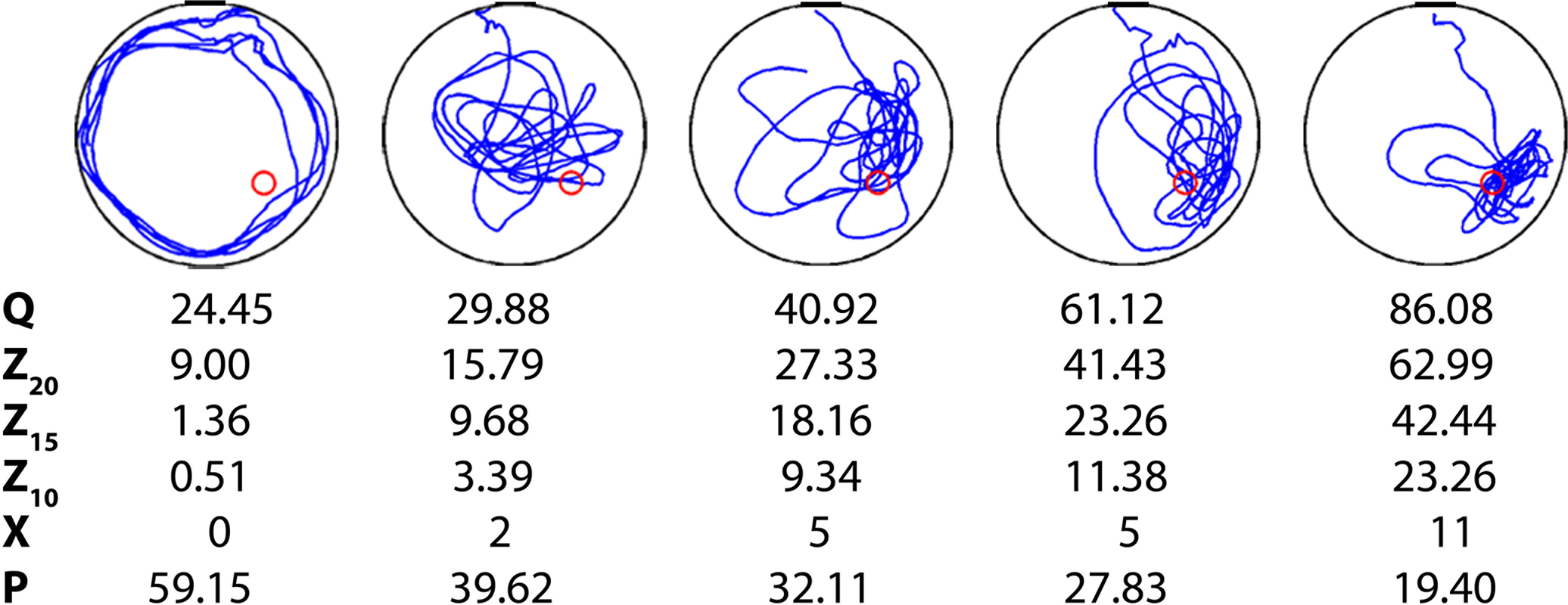
Figure 1. Examples of five individual probe tests. Mice were trained in the water maze with six trials per day for 5 days. Shown are representative swim paths in a probe test conducted following the completion of training. Corresponding quantification of probe test performance is shown below for the four widely used probe test measures: quadrant (Q), zone (Z20, Z15, Z10), crossings (X) and proximity (P).
Apparatus and Behavioral Methods
Apparatus
All water maze experiments were conducted in a circular tank (120 cm in diameter, 50 cm deep), located in a dimly-lit room (Kee et al., 2007a
,b
; Teixeira et al., 2006
). The pool was filled to a depth of 40 cm with water made opaque by adding white non-toxic paint. Water temperature, monitored by a thermometer located 20 cm below the water surface, was maintained at 28 ± 1°C by a heating pad located beneath the pool. A circular escape platform (5 cm radius) was submerged 0.5 cm below the water surface and located in the south-east quadrant. The pool was surrounded by curtains, at least 1 m from the perimeter of the pool. The curtains were white, and had distinct cues painted on them.
Training procedures
Prior to the commencement of training, mice were individually handled for 2 min each day for 1 week. On each training day, mice received six training trials (presented in two blocks of three trials; inter-block interval of ∼1 h, inter-trial interval was ∼15 s). On each trial they were placed into the pool, facing the wall, in one of four start locations (north, south, east, west). The order of these start locations was pseudo-randomly varied throughout training. The trial was complete once the mouse found the platform or 60 s had elapsed. If the mouse failed to find the platform on a given trial, the experimenter guided the mouse onto the platform.
Probe test procedures
During the probe test, mice were placed into the pool facing the wall, in the north location. The probe test was 60 s in duration.
Quantification of probe test performance
Behavioral data from the probe tests were acquired and analyzed using an automated tracking system (Actimetrics, Wilmette, IL, USA). Using this software, the precise mouse location (in x, y coordinates) was recorded throughout the probe test (capture rate 10 frames/s). From this spatial distribution, the following performance measures were calculated automatically:
1. Percent quadrant time (Q). Amount of time mice searched a virtual quadrant (i.e., 25% of total pool surface area), centered on the location of the platform during training (Morris, 1981
, 1984
; Morris et al., 1982
).
2. Percent zone. Amount of time mice searched virtual target zones (20 [Z20], 15 [Z15] and 10 [Z10] cm in radius, centered on the location of the platform during training) during the 60-s test (de Hoz et al., 2004
; Moser and Moser, 1998
; Moser et al., 1993
). These zones represent 1/9th (∼11.1%), 1/16th (∼6.25%) and 1/36th (∼2.8%) of the total pool surface area, respectively.
3. Crossings (X). Number of times mice cross the exact location of the platform (5 cm in radius) during the 60-s test (Morris, 1981
, 1984
; Morris et al., 1982
).
4. Proximity (P) measure (Gallagher’s measure) (Gallagher et al., 1993
). Average distance in centimeters of mice from center of the platform location across the 60-s test.
These measures (or combinations thereof) are used to quantify probe test performance in more than 98% of published papers (Figure 2
).
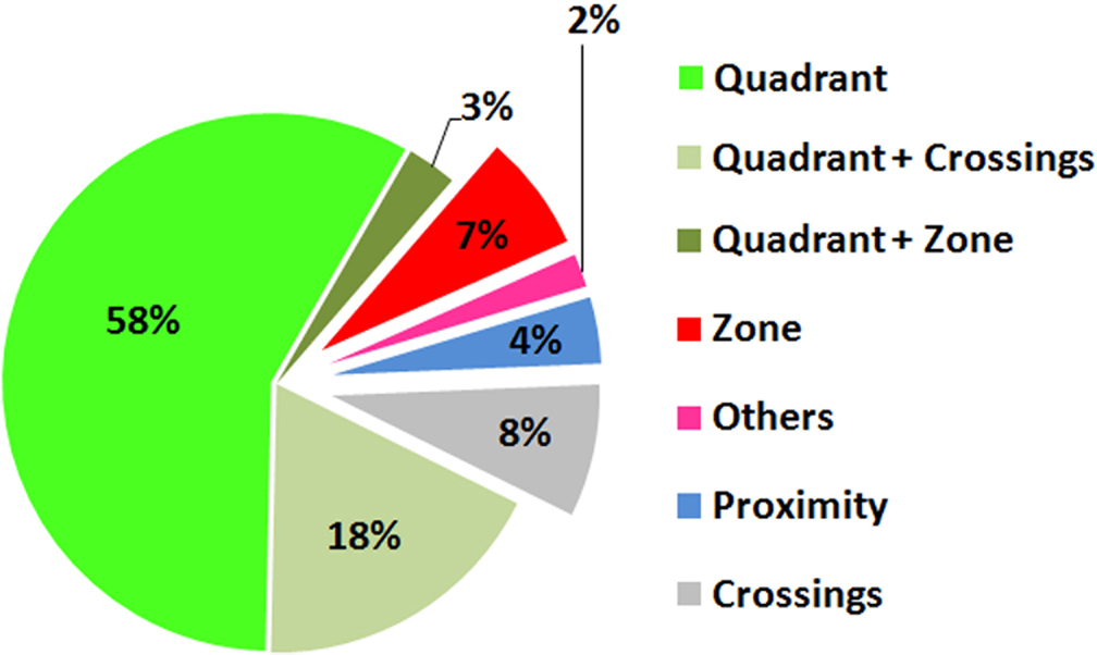
Figure 2. Popularity of different probe test measures. To assess the relative frequency with which different probe test measures are used, a PubMed search (http://www.ncbi.nlm.nih.gov/sites/entrez
) using the terms [(rat OR mouse) AND water maze] was conducted for the period 2004–2006. Out of a total of 205 papers surveyed, 135 assessed spatial learning/memory using a probe test. The pie chart shows the relative frequency that different measures (or combinations of measures) were used to quantify probe test performance in these studies.
Data Sets
Probe test data were pooled from experiments conducted in our laboratory between June 2004 and June 2008. All experiments were conducted using identical apparatus, training and probe test procedures, as described above. Procedures were approved by the Animal Care Committee at Hospital for Sick Children.
Analysis A
In the first analysis, probe test data were pooled from experiments where wild-type mice were initially trained for 5 days (six trials per day) and then given a probe test at variable delays following the completion of training. These experiments examined the impact of different genetic, pharmacological and neuroanatomical lesion manipulations on water maze performance (for details see Kee et al., 2007b
; Teixeira et al., 2006
; Wang et al., 2009
). For these analyses, probe test data were divided into two data sets. First, a control data set (n = 370 probe tests) that included data from control mice in the genetic (i.e., wild-type mice), pharmacological (i.e., mice received control infusions of phosphate-buffered saline) and neuroanatomical lesion (i.e., sham surgery) experiments. Second, an experimental data set (n = 388 probe tests) that included data from experimental mice in the genetic [e.g., α-CaMKIIT286A knockin mice (Giese et al., 1998
; Kee et al., 2007b
)], pharmacological [e.g., mice received lidocaine infusion into the dorsal hippocampus prior to testing (Teixeira et al., 2006
)] and neuroanatomical lesion [i.e., NMDA-induced complete hippocampal lesion (Wang et al., 2009
)] experiments. All mice used in these and subsequent experiments were in a mixed C57Bl/6NTacfBr [C57B6] and 129Svev [129] background (50:50) (Taconic, Germantown, NY, USA). In the majority of experiments, these were the F1 generation. In a subset of experiments, the F2 generation was used. The mean and standard deviation for the control and experimental datasets are shown in Figure 3
A.
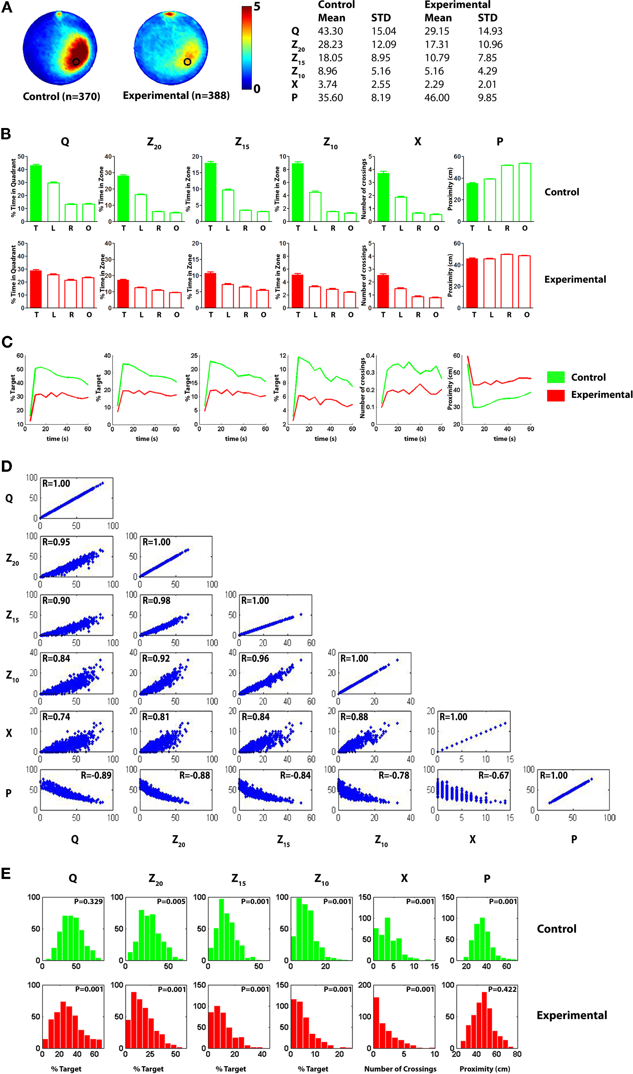
Figure 3. Pooled probe test data for control and experimental mice for analysis A. (A) Left, density plots for grouped data showing where control and experimental mice concentrated their searches in the probe test. The color scale represents the mean number of visits per animal per 5 cm × 5 cm area. Right, summary of descriptive statistics (mean values, standard deviations) for the target quadrant (Q), zone (Z20, Z15 and Z10), crossing (X) and proximity (P) measures for control and experimental datasets. (B) Comparison of target (T) vs. other pseudo-platform locations (right, R; left, L; opposite, O) for each measure (upper graphs show control data, lower graphs experimental data). (C) Temporal profile of spatial bias across 60 s probe test for quadrant (Q), zone (Z20, Z15 and Z10), crossing (X) and proximity (P) measures. Averaged data are shown in 5 s bins for control (green) and experimental (red) datasets. (D) Scatterplots illustrating how respective water maze measures correlate with one another for all 758 probe tests included in the control and experimental datasets. Measures tended to be highly correlated, with r-values range from 0.67 to 0.98 (all P-values <0.01). (E) Distribution of probe test scores for control (upper; green) and experimental (lower; red) datasets for each measure. According to the Lilliefors (Kolmogorov–Smirnov) test, many distributions are positively skewed (P-values <0.05).
Analysis B
In the second analysis, probe test data were pooled from experiments where wild-type mice (n = 282) were trained for 5 days with six trials per day. At variable delays following the completion of training, they received a series of three consecutive probe tests. Performance declined across probe tests, most likely reflecting extinction of spatial memory (Lattal et al., 2003
). The decline in performance therefore provides three datasets with three distinct levels of performance (see Figure 5
A).
Quantitative and Statistical Analyses
Datasets used for analyses A and B were exported to Matlab (http://www.mathworks.com/products/matlab/
) and Q, Z20, Z15, Z10, X and P were computed for each individual trajectory. For each dataset, descriptive statistics (mean, standard deviation) were computed. Additionally, for the control and experimental datasets used in analysis A, between-measure correlations (Pearson’s r) were computed and the Lilliefors [Kolmogorov–Smirnov (K–S)] test was used to evaluate whether measures were normally distributed.
In order to compare the sensitivity of the different measures at detecting experimental effects a series of simulated experiments were conducted. For analysis A, N (range 5–40) probe tests were randomly selected (without replacement) from the control and experimental datasets, respectively. Whether the two samples differed was then evaluated using either a parametric (Student’s t-test) or non-parametric (K–S test) statistic
1
. For each N, 1000 simulations were conducted and, to compute the rate of rejection of the null hypothesis for each N, 10 replications were performed. In order to evaluate the false-positive rate, the above analyses were repeated, but both samples were drawn from the control dataset (again without replacement). All analyses were conducted with α set at 0.05, 0.01 and 0.005, respectively. For analysis B, a similar series of simulations were conducted to compare the probe 1, 2 and 3 datasets.
Control vs. Experimental (Analysis A, Descriptive Statistics)
Pooled probe test data for control (n = 370) and experimental (n = 388) mice are shown in Figure 3
. These probe tests were conducted using identical experimental procedures in the same apparatus in our behavioral laboratory at The Hospital for Sick Children, Toronto, between 2004 and 2008. The analyses in this paper are focused on comparing bias for the target location between groups. The heat maps indicate that control mice (compared to experimental mice) searched more extensively around the target location (i.e., the former platform location) (Figure 3
A), and this superior performance is captured by all measures (Table to right of Figure 3
A). It is also possible to contrast bias for the target location (e.g., south-east) with other equivalent locations in the pool (e.g., north-east, north-west and south-west), and this within-subjects comparison is shown in Figure 3
B.
To examine how the precision of spatial searches changes over the course of the probe trial, we divided the probe test into 5 s bins. According to the Q, Z20, Z15, Z10 and P measures, search precision initially rose sharply, peaked between 10–15 s, and then declined thereafter (Figure 3
C). Mice began each probe test from a start position that was opposite to the target location, and so this likely accounts for the rapid rise in search precision. The subsequent decline in search precision likely reflects within-test extinction (Lattal et al., 2003
; Suzuki et al., 2004
). The temporal profile of the X measure differed from other measures: Crossing probability exhibited the same initial sharp increase, but was then relatively stable thereafter.
We next examined how well the measures correlated with one another (Figure 3
D). As would be expected, the measures were significantly correlated with one another (all P-values <0.01), with Pearson’s r ranging from 0.67 (X vs. P) to 0.98 (Z20 vs. Z15). Correlation coefficients were generally highest between the various occupancy-based measures (Q, Z20, Z15 and Z10; 0.84–0.98), and lowest for contrasts that included X (0.67–0.88).
Parametric tests (such as the Student’s t-test or ANOVA) are based on the assumption that samples are drawn from populations that are normally distributed
2
. We therefore next evaluated whether the measures were normally distributed using the Lilliefors (K–S) test. These analyses revealed that the measures were not normally distributed, in the majority of cases, tending to be positively skewed (Figure 3
E). This was most pronounced in the experimental condition, most likely because many of these mice are performing at, or near, floor levels (i.e., mode for Q ≈ 20.4–27.2%, X = 0).
Analysis A, Hypothesis Testing
We next conducted a series of simulated experiments to compare the sensitivity of the different measures at detecting differences between the control and experimental groups. Experiments were simulated by randomly selecting N probe tests (without replacement) from the control and experimental groups respectively, and testing for group differences for each of the six measures using the Student’s t-test. For each N, 1000 simulations were conducted and, to compute the rate of rejection of the null hypothesis for each N, 10 replications were performed (Figure 4
A, left). As group size increased, the detection rates increased for all measures. For Ns up to around 40, we found that detection rates were highest for P compared to Q, Z and X, respectively. For example, with α set at 0.05 and N = 15, group differences were more frequently detected using P (∼86%) compared to Q (∼70%) for Z20 (∼70%), Z15 (∼63%), Z10 (∼57%) and X (∼39%). The relative advantage of P over Q, Z and X held with α set at 0.01 and 0.005.
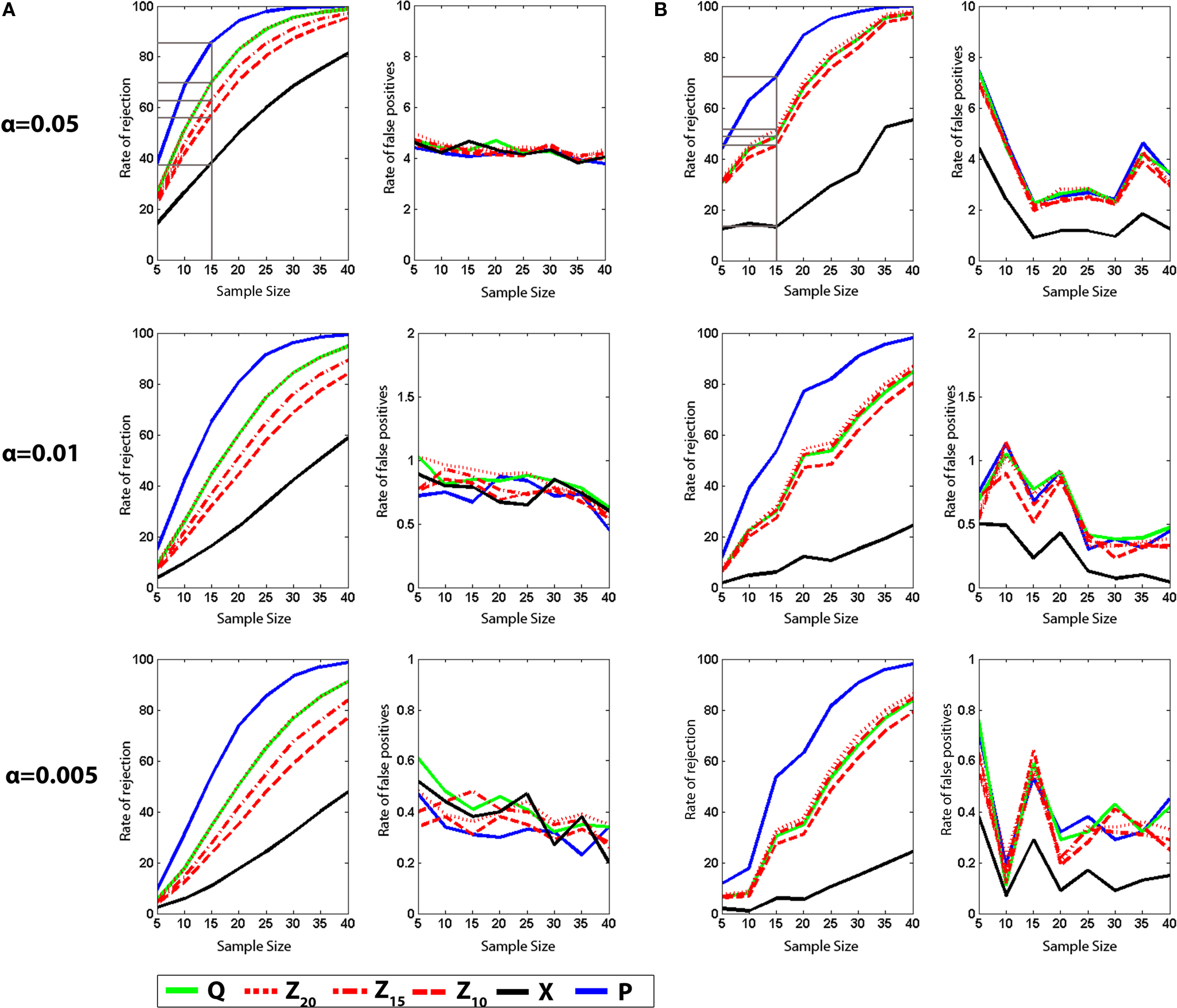
Figure 4. Monte Carlo simulations (analysis A). (A) t-tests. Left, the likelihood of detecting a difference between control and experimental groups is shown for varying sample (N) size, with significance levels α = 0.05, 0.01 and 0.005. Right, false-positive rates when both samples are drawn from the control dataset.
(B) K–S tests. Left, the likelihood of detecting a difference between control and experimental groups is shown for varying sample (N) size, with significance levels α = 0.05, 0.01 and 0.005. Right, false-positive rate when both samples are drawn from the control dataset. Q (green), Z (red; Z20, Z15 and Z10), X (black) and P (blue).
With α set at 0.05 in the above simulations we would expect a false-positive rate of ∼5%. To verify that false-positive rates were as expected we performed the same analyses as above, but randomly selected two groups of N probe tests from the same control population (Figure 4
A, right). For low Ns, false-positive rates were at expected levels when α was set at 0.05, 0.01 and 0.005, respectively. As Ns increased false-positive rates tended to decline, however. This decline is most likely because our control database contains a finite number of probe tests (i.e., 370). Therefore, as N increases (and approaches this finite value), so does the likelihood that some of the same data-points will be selected in both the first and second samples and such duplication would naturally reduce the likelihood that the two groups differ.
An assumption of parametric statistics such as the Student’s t-test is that the two samples are drawn from normally distributed populations. Our analyses presented in Figure 3
D suggest that this may not always be the case in water probe test data, regardless of which of the four measures are being used. Therefore, to address this issue we next performed an identical series of simulations but used a non-parametric statistic (K–S test) that makes no assumptions about the underlying distributions of the two samples (Figure 4
B, left). As would be expected using this more conservative statistical approach, overall detection rates were lower. Importantly, however, P maintained its advantage over other measures: Again, with α set at 0.05 and N = 15, P was considerably more successful at detecting group differences (∼72%) compared to Q (∼49%) for Z20 (∼52%), Z15 (∼49%), Z10 (∼45%) and X (∼13%). False-positive rates were similar across measures and close to expected values (Figure 4
B, right).
Analysis B, Hypothesis Testing for Varying Effect Sizes
The probability of rejecting the null hypothesis (and detecting a difference) depends upon the effect size (i.e., difference between means), as well as the sample size (N) and the variance of the samples. As we sampled from two populations in the above analyses, the effect size was fixed (i.e., QC – QE ≈ 14%, XC – XE ≈ 1.45). In order to examine the sensitivity of different measures at detecting intermediate effect sizes we compiled three additional databases, each containing ≥282 probe tests. These databases were compiled from mice that had all been trained identically (5 days, six trials per day) and then given a series of three probe tests. Performance differed in each of the probe trials (declining from probe 1 → 3, likely reflecting within session extinction). Therefore, comparison of different combinations of probe tests provides an opportunity to evaluate the ability of the different measures to detect differences over a range of intermediate effect sizes (Figure 5
A). Accordingly, we next performed a series of simulated experiments (as above) and tested for differences using both parametric (t-test) and non-parametric (K–S test) statistics (Figures 5
B,C). As in our previous analyses, as N increased, detection rates increased for all measures. In two of the three comparisons, P outperformed Q, Z and X (probe 1 vs. probe 3 and probe 1 vs. probe 2). However, for the probe 2 vs. probe 3 comparison, Z20, Z15 and Z10 were most sensitive. This suggests that the advantage of P over other measures may not be universal: In situations where both groups are performing poorly, Z-based measures may be superior. One possible reason for the poor performance of P for the probe 2 vs. probe 3 comparison is that when mice are performing close to chance levels (e.g., swimming around the perimeter of the pool), variance for P would be especially high, thereby reducing the likelihood of detecting group differences. False-positive rates were similar across measures and close to expected values for both t-tests and K–S tests.
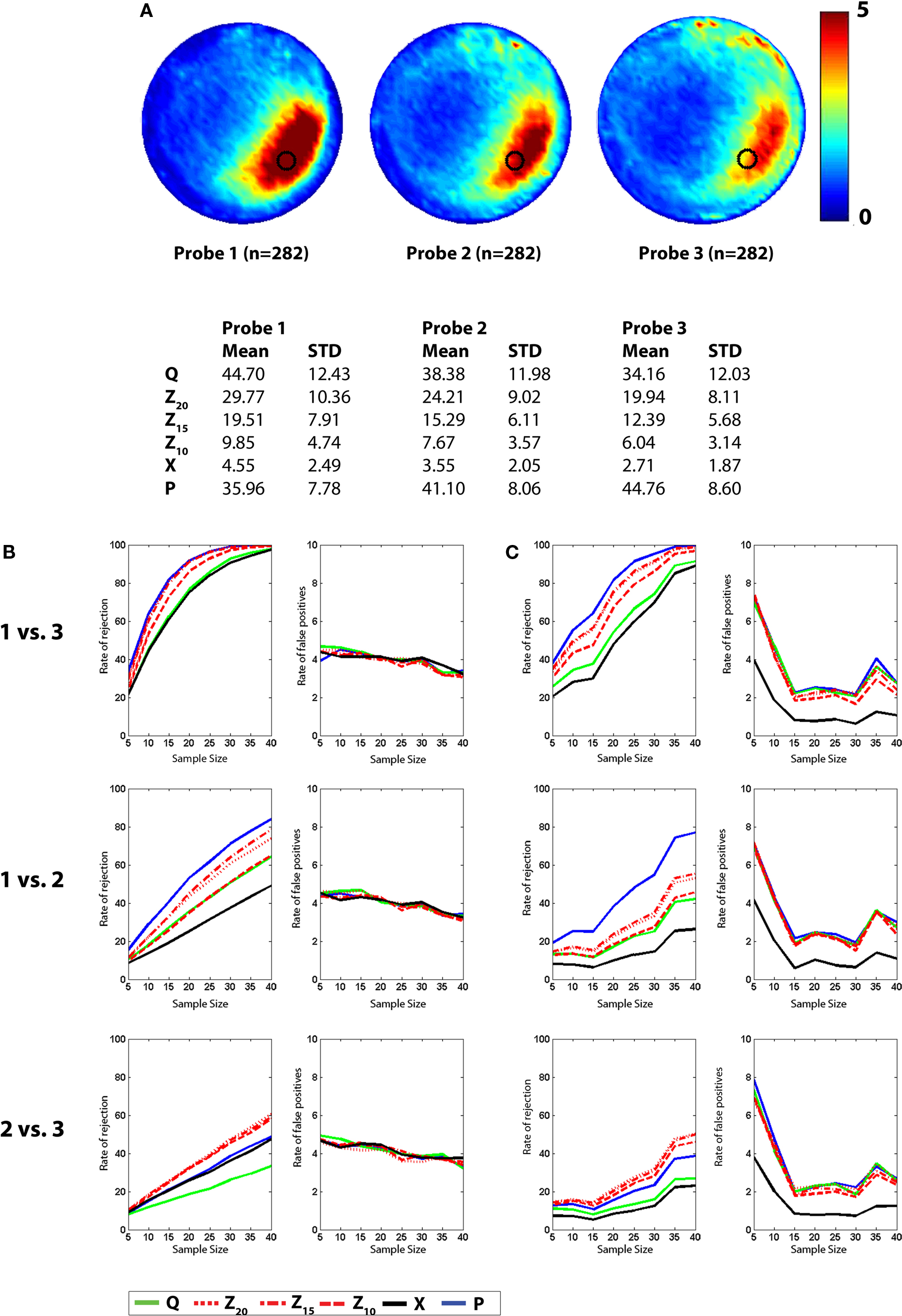
Figure 5. Monte Carlo simulations (analysis B). Mice were trained in the water maze for 5 days (six trials per day) and then given a series of three probe tests. (A) Density plots for grouped data showing probes 1, 2 and 3. The color scale represents the number of visits per animal per 5 cm × 5 cm area. The table below indicates that performance declined across probe tests, according to all measures. (B) t-tests. Left, the likelihood of detecting a difference between the probe 1, 2 and 3 datasets is shown for varying sample (N) size, with significance levels α = 0.05. Right, false-positive rates when both samples are drawn from the same dataset. (C) K–S tests. Left, the likelihood of detecting a difference between the probe 1, 2 and 3 datasets is shown for varying sample (N) size, with significance levels α = 0.05. Right, false-positive rates when both samples are drawn from the same dataset. Q (green), Z (red; Z20, Z15 and Z10), X (black) and P (blue).
In assessing probe test performance in the water maze, four measures are routinely used to assess search accuracy (quadrant [Q], zone [Z], crossings [X] and proximity [P]). Using databases containing more than 1600 individual probe tests we conducted a series of Monte Carlo simulations to compare the relative sensitivity of these four measures in detecting group differences. Our primary finding is that P outperformed Z, Q and X, respectively. This was the case across a range of sample sizes and for most effect sizes, and whether parametric or non-parametric analyses were used. While the water maze has been extensively validated, and all major findings reliably replicated across labs, the sensitivity of measures used to assess performance have received less attention. Here, our formal evaluation of sensitivity suggests the use of the P measure may facilitate more efficient detection of spatial learning phenotypes in mice by reducing mouse numbers and increasing throughput.
The four measures that we focused on have been used in more than 98% of water maze studies (Figure 1
) and fall into three subcategories. First, occupancy-based measures assess the amount of time animals spend in a virtual area (quadrant or zone) that is centered on the former platform location. The crossing measure is a counting-based measure where the number of times an animal crosses the exact former location of the platform is recorded. Finally, proximity is an error-based measure where the animal’s average distance from the former platform location is recorded. Common to each of these measures is that bias for the target location (e.g., south-east) may be contrasted with other equivalent locations in the pool (e.g., north-east, north-west and south-west). Such a within-subjects comparison makes it possible to assess whether a particular cohort of mice search selectively (e.g., whether they search more in the south-east quadrant relative to the north-east, north-west and south-west quadrants). However, as both control and experimental groups may both search selectively, the critical comparison is whether one group searches more selectively than the other. For this between subjects comparison, relative bias for the target (Q, Z, X, P) must be contrasted between control and experimental groups, and this is the comparison that we focused on in this study.
Our surprising finding was that the least popular of the four measures – proximity (Gallagher et al., 1993
) – was consistently more sensitive at detecting group differences. What might account for increased sensitivity of proximity measure? The two most popular measures – quadrant and crossings – were introduced in the original water maze studies (Morris, 1981
, 1984
; Morris et al., 1982
) at a time when more sophisticated tracking analysis was not available. While offering considerable intuitive appeal – for example, it is readily apparent that an animal searching non-selectively would be expected to spend around 25% of its time in each quadrant – nonetheless these two measures make use of only very impoverished spatial information. That is, quadrant (along with zone) simply calculates the proportion of time an animal spends in one location (or crosses that location), discarding all other spatial information. Contemporary tracking systems contain precise, moment-by-moment spatial information and much of this detail is retained in the proximity computation. The future development of more sensitive measures to assess search accuracy in water maze probe tests will likely further exploit the richness of this spatial distribution and therefore offer greater sensitivity (e.g., Dvorkin et al., 2008
; Valente et al., 2007
).
The analysis of a large number of probe trials allowed us to examine the temporal pattern of searching in some detail. The most interesting observation is that search accuracy in control mice peaked between 10 and 15 s, and declined thereafter (as measured by Q, Z and P, but not X). This within-test extinction suggests that relatively early on in the probe test mice learn that the platform is absent and shift strategy to search elsewhere. The exact timing of this peak likely depends on several factors, including the amount of training and the type of escape platform used during training [standard vs. Atlantis (de Hoz et al., 2004
)] and might in itself provide an informative index of cognitive function (or ‘certainty’).
Finally, our databases were composed of probe test data that were drawn from experiments using identical apparatus, training and probe test procedures. An advantage of this approach, therefore, is that our simulated experiments closely mimic real experimental situations, as for any given experiment such factors would typically not vary. However, one disadvantage is also worth noting. The drawback of using identical procedures is that it is unclear whether the relative ranking of P, Z, Q and X would necessarily hold across a variety of experimental settings. For example, many factors commonly differ across laboratories. These include pool size, size and type of platform, amount of training, external cues, strain and species, all of which impact performance. While we believe it is reasonable to assume that the general ranking of measures would generalize across experimental settings, nonetheless it be would be important establish this in future analyses.
The authors declare that the research was conducted in the absence of any commercial or financial relationships that could be construed as a potential conflict of interest.
This work was supported by a grant from the Natural Sciences and Engineering Council Canada [RGPIN 312434-05] (PWF). Hamid R. Maei received support from the Research Training Centre at The Hospital for Sick Children. Cátia M. Teixeira received support from the Graduate Program in Areas of Basic and Applied Biology (GABBA) and the Portuguese Foundation for Science and Technology (FCT). We thank Adrienne Yeung for compiling the PubMed analysis, and Sheena Josselyn, Noam Miller, Steven Kushner and Ilya Zaslavsky for comments on earlier drafts of this manuscript.
- ^ For example, for the control dataset, 10 probe tests (out of 370) were randomly selected. These were then compared to 10 (out of 388) randomly selected probe tests from the experimental database (the control and experimental databases are composed of multiple actual experiments conduced in the lab between 2004 and 2008).
- ^ Violations of this normality assumption will lead to a modest increase in the Type I error rate (i.e., incorrectly rejecting the null hypothesis). Such effects would be most pronounced for smaller sample sizes (i.e., ns < 40) and when sample distributions are differently shaped (Sawilowsky and Hillman, 1992 ).
Chapman, P. F., White, G. L., Jones, M. W., Cooper-Blacketer, D., Marshall, V. J., Irizarry, M., Younkin, L., Good, M. A., Bliss, T. V., Hyman, B. T., Younkin, S. G., and Hsiao, K. K. (1999). Impaired synaptic plasticity and learning in aged amyloid precursor protein transgenic mice. Nat. Neurosci. 2, 271–276.